Solar Cycle (SOLAR)SOLAR: SOLAR CYCLE
🔍 OVERVIEW AND PURPOSE
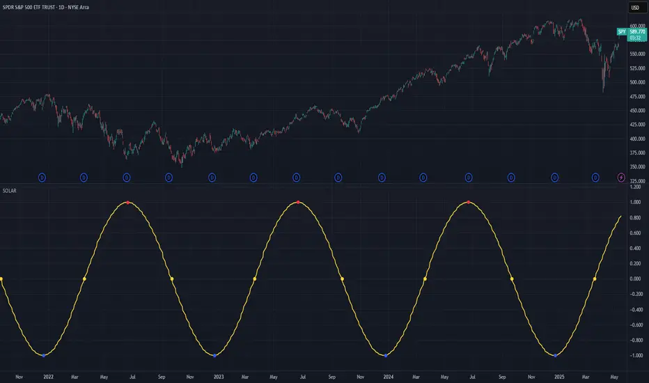
The Solar Cycle indicator is an astronomical calculator that provides precise values representing the seasonal position of the Sun throughout the year. This indicator maps the Sun's position in the ecliptic to a normalized value ranging from -1.0 (winter solstice) through 0.0 (equinoxes) to +1.0 (summer solstice), creating a continuous cycle that represents the seasonal progression throughout the year.
The implementation uses high-precision astronomical formulas that include orbital elements and perturbation terms to accurately calculate the Sun's position. By converting chart timestamps to Julian dates and applying standard astronomical algorithms, this indicator achieves significantly greater accuracy than simplified seasonal approximations. This makes it valuable for traders exploring seasonal patterns, agricultural commodities trading, and natural cycle-based trading strategies.
🧩 CORE CONCEPTS
Seasonal cycle integration: Maps the annual solar cycle (365.242 days) to a continuous wave
Continuous phase representation: Provides a normalized -1.0 to +1.0 value
Astronomical precision: Uses perturbation terms and high-precision constants for accurate solar position
Key points detection: Identifies solstices (±1.0) and equinoxes (0.0) automatically
The Solar Cycle indicator differs from traditional seasonal analysis tools by incorporating precise astronomical calculations rather than using simple calendar-based approximations. This approach allows traders to identify exact seasonal turning points and transitions with high accuracy.
⚙️ COMMON SETTINGS AND PARAMETERS
Pro Tip: While the indicator itself doesn't have adjustable parameters, it's most effective when used on higher timeframes (daily or weekly charts) to visualize seasonal patterns. Consider combining it with commodity price data to analyze seasonal correlations.
🧮 CALCULATION AND MATHEMATICAL FOUNDATION
Simplified explanation:
The Solar Cycle indicator calculates the Sun's ecliptic longitude and transforms it into a sine wave that peaks at the summer solstice and troughs at the winter solstice, with equinoxes at the zero crossings.
Technical formula:
Convert chart timestamp to Julian Date:
JD = (time / 86400000.0) + 2440587.5
Calculate Time T in Julian centuries since J2000.0:
T = (JD - 2451545.0) / 36525.0
Calculate the Sun's mean longitude (L0) and mean anomaly (M), including perturbation terms:
L0 = (280.46646 + 36000.76983T + 0.0003032T²) % 360
M = (357.52911 + 35999.05029T - 0.0001537T² - 0.00000025T³) % 360
Calculate the equation of center (C):
C = (1.914602 - 0.004817T - 0.000014*T²)sin(M) +
(0.019993 - 0.000101T)sin(2M) +
0.000289sin(3M)
Calculate the Sun's true longitude and convert to seasonal value:
λ = L0 + C
seasonal = sin(λ)
🔍 Technical Note: The implementation includes terms for the equation of center to account for the Earth's elliptical orbit. This provides more accurate timing of solstices and equinoxes compared to simple harmonic approximations.
📈 INTERPRETATION DETAILS
The Solar Cycle indicator provides several analytical perspectives:
Summer Solstice (+1.0): Maximum solar elevation, longest day
Winter Solstice (-1.0): Minimum solar elevation, shortest day
Vernal Equinox (0.0 crossing up): Day and night equal length, spring begins
Autumnal Equinox (0.0 crossing down): Day and night equal length, autumn begins
Transition rates: Steepest near equinoxes, flattest near solstices
Cycle alignment: Market cycles that align with seasonal patterns may show stronger trends
Confirmation points: Solstices and equinoxes often mark important seasonal turning points
⚠️ LIMITATIONS AND CONSIDERATIONS
Geographic relevance: Solar cycle timing is most relevant for temperate latitudes
Market specificity: Seasonal effects vary significantly across different markets
Timeframe compatibility: Most effective for longer-term analysis (weekly/monthly)
Complementary tool: Should be used alongside price action and other indicators
Lead/lag effects: Market reactions to seasonal changes may precede or follow astronomical events
Statistical significance: Seasonal patterns should be verified across multiple years
Global markets: Consider opposite seasonality in Southern Hemisphere markets
📚 REFERENCES
Meeus, J. (1998). Astronomical Algorithms (2nd ed.). Willmann-Bell.
Hirshleifer, D., & Shumway, T. (2003). Good day sunshine: Stock returns and the weather. Journal of Finance, 58(3), 1009-1032.
Hong, H., & Yu, J. (2009). Gone fishin': Seasonality in trading activity and asset prices. Journal of Financial Markets, 12(4), 672-702.
Bouman, S., & Jacobsen, B. (2002). The Halloween indicator, 'Sell in May and go away': Another puzzle. American Economic Review, 92(5), 1618-1635.
Penunjuk Pine Script®