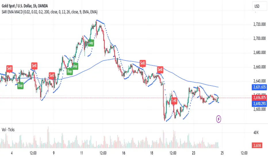
Parabolic SAR + EMA 200 + MACD SignalsParabolic SAR + EMA 200 + MACD Signals Indicator, a powerful tool designed to help traders identify optimal entry points in the market.
This indicator combines three popular technical indicators: Parabolic SAR (Stop and Reverse), EMA200 (Exponential Moving Average 200) and MACD (Moving Average Convergence Divergence) - to provide clear and concise buy and sell signals based on market trends.
The MACD component of this indicator calculates the difference between two exponentially smoothed moving averages, providing insight into the trend strength of the market. The Parabolic SAR component helps identify potential price reversals, while the EMA200 acts as a key level of support and resistance, providing additional confirmation of the overall trend direction.
Whether you're a seasoned trader or just starting out, the MACD-Parabolic SAR-EMA200 Indicator is a must-have tool for anyone looking to improve their trading strategy and maximize profits in today's dynamic markets.
Buy conditions
The price should be above the EMA 200
Parabolic SAR should show an upward trend
MACD Delta should be positive
ُSell conditions
The price should be below the EMA 200
Parabolic SAR should show an downward trend
MACD Delta should be negative
Cari dalam skrip untuk "Exponential"
Simple_RSI+PA+DCA StrategyThis strategy is a result of a study to understand better the workings of functions, for loops and the use of lines to visualize price levels. The strategy is a complete rewrite of the older RSI+PA+DCA Strategy with the goal to make it dynamic and to simplify the strategy settings to the bare minimum.
In case you are not familiar with the older RSI+PA+DCA Strategy, here is a short explanation of the idea behind the strategy:
The idea behind the strategy based on an RSI strategy of buying low. A position is entered when the RSI and moving average conditions are met. The position is closed when it reaches a specified take profit percentage. As soon as the first the position is opened multiple PA (price average) layers are setup based on a specified percentage of price drop. When the price hits the layer another position with the same position size is is opened. This causes the average cost price (the white line) to decrease. If the price drops more, another position is opened with another price average decrease as result. When the price starts rising again the different positions are separately closed when each reaches the specified take profit. The positions can be re-opened when the price drops again. And so on. When the price rises more and crosses over the average price and reached the specified Stop level (the red line) on top of it, it closes all the positions at once and cancels all orders. From that moment on it waits for another price dip before it opens a new position.
This is the old RSI+PA+DCA Strategy:
The reason to completely rewrite the code for this strategy is to create a more automated, adaptable and dynamic system. The old version is static and because of the linear use of code the amount of DCA levels were fixed to max 6 layers. If you want to add more DCA layers you manually need to change the script and add extra code. The big difference in the new version is that you can specify the amount of DCA layers in the strategy settings. The use of 'for loops' in the code gives the possibility to make this very dynamic and adaptable.
The RSI code is adapted, just like the old version, from the RSI Strategy - Buy The Dips by Coinrule and is used for study purpose. Any other low/dip finding indicator can be used as well
The distance between the DCA layers are calculated exponentially in a function. In the settings you can define the exponential scale to create the distance between the layers. The bigger the scale the bigger the distance. This calculation is not working perfectly yet and needs way more experimentation. Feel free to leave a comment if you have a better idea about this.
The idea behind generating DCA layers with a 'for loop' is inspired by the Backtesting 3commas DCA Bot v2 by rouxam .
The ideas for creating a dynamic position count and for opening and closing different positions separately based on a specified take profit are taken from the Simple_Pyramiding strategy I wrote previously.
This code is a result of a study and not intended for use as a full functioning strategy. To make the code understandable for users that are not so much introduced into pine script (like myself), every step in the code is commented to explain what it does. Hopefully it helps.
Enjoy!

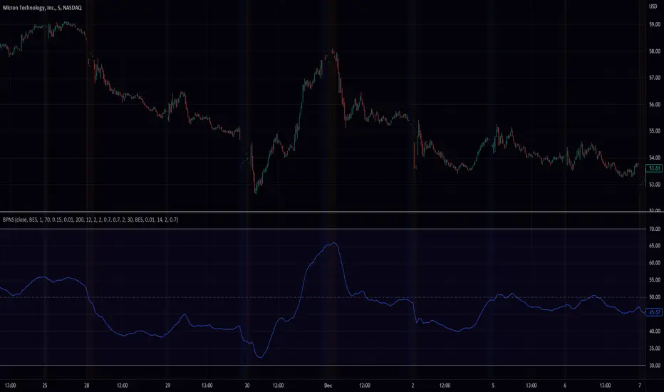
Band Pass Normalized Suite (BPNS)Outlier-Free Normalization and Band Pass Filtering
We present a technique for normalizing and filtering a given time series, source, in order to improve its stationarity and enhance its features. The technique includes two stages: outlier-free normalization and band pass filtering.
Outlier-Free Normalization:
In order to normalize source and reduce the impact of outliers, we first smooth the time series using an exponential moving average with a smoothing factor of alpha. The smoothed time series is then normalized by subtracting the minimum value within a given lookback period, dev_lookback, and dividing the result by the range (maximum - minimum) within the same lookback period. Outliers are detected and excluded from the normalization process by identifying values that are more than outlier_level standard deviations away from the exponentially smoothed average.
Band Pass Filtering:
After normalization, the time series is passed through a band pass filter to remove low and high frequency components. The specifics of the band pass filter implementation are not provided.
Code snippet:
bes(float source = close, float alpha = 0.7) =>
var float smoothed = na
smoothed := na(smoothed) ? source : alpha * source + (1 - alpha) * nz(smoothed )
max(source, outlier_level, dev_lookback)=>
var float max = na
src = array.new()
stdev = math.abs((source - bes(source, 0.1))/ta.stdev(source, dev_lookback))
array.push(src, stdev < outlier_level ? source : -1.7976931348623157e+308)
max := math.max(nz(max ), array.get(src, 0))
min(source, outlier_level, dev_lookback) =>
var float min = na
src = array.new()
stdev = math.abs((source - bes(source, 0.1))/ta.stdev(source, dev_lookback))
array.push(src, stdev < outlier_level ? source : 1.7976931348623157e+308)
min := math.min(nz(min ), array.get(src, 0))
min_max(src, outlier_level, dev_lookback) =>
(src - min(src, outlier_level, dev_lookback))/(max(src, outlier_level, dev_lookback) - min(src, outlier_level, dev_lookback)) * 100
To apply the outlier-free normalization and band pass filter to a given time series, source, the min_max() function can be called with the desired values for outlier_level and dev_lookback as arguments. For example:
normalized_source = min_max(source, 2, 50)
This will apply the outlier-free normalization and band pass filter to source, using an outlier_level of 2 standard deviations and a lookback period of 50 data points for both the normalization and outlier detection steps. The resulting normalized and filtered time series will be stored in normalized_source.
It is important to note that the choice of values for outlier_level and dev_lookback will have a significant impact on the resulting normalized and filtered time series. These values should be chosen carefully based on the characteristics of the input time series and the desired properties of the normalized and filtered output.
In conclusion, the outlier-free normalization and band pass filtering technique presented here provides a useful tool for preprocessing time series data and improving its stationarity and feature content. The flexibility of the method, through the choice of outlier_level and dev_lookback values, allows it to be tailored to the specific characteristics of the input time series.
AMASling - All Moving Average Sling ShotThis indicator modifies the SlingShot System by Chris Moody to allow it to be based on 'any' Fast and Slow moving average pair. Open Long / Close Long / Open Short / Close Short alerts can be generated for automated bot trading based on the SlingShot strategy:
• Conservative Entry = Fast MA above Slow MA, and previous bar close below Fast MA, and current price above Fast MA
• Conservative Entry = Fast MA below Slow MA, and previous bar close above Fast MA, and current price below Fast MA
• Aggressive Entry = Fast MA above Slow MA, and price below Fast MA
• Aggressive Exit = Fast MA below Slow MA, and price above Fast MA
Entries and exits can also be made based on moving average crossovers, I initially put this in to make it easy to compare to a more standard strategy, but upon backtesting combining crossovers with the SlingShot appeared to produce better results on some charts.
Alerts can also be filtered to allow long deals only when the fast moving average is above the slow moving average (uptrend) and short deals only when the fast moving average is below the slow moving averages (downtrend).
If you have a strategy that can buy based on External Indicators you can use the 'Backtest Signal' which plots the values set in the 'Long / Short Signals' section.
The Fast, Slow and Signal Moving Averages can be set to:
• Simple Moving Average (SMA)
• Exponential Moving Average (EMA)
• Weighted Moving Average (WMA)
• Volume-Weighted Moving Average (VWMA)
• Hull Moving Average (HMA)
• Exponentially Weighted Moving Average (RMA) (SMMA)
• Linear regression curve Moving Average (LSMA)
• Double EMA (DEMA)
• Double SMA (DSMA)
• Double WMA (DWMA)
• Double RMA (DRMA)
• Triple EMA (TEMA)
• Triple SMA (TSMA)
• Triple WMA (TWMA)
• Triple RMA (TRMA)
• Symmetrically Weighted Moving Average (SWMA) ** length does not apply **
• Arnaud Legoux Moving Average (ALMA)
• Variable Index Dynamic Average (VIDYA)
• Fractal Adaptive Moving Average (FRAMA)
'Backtest Signal' and 'Deal State' are plotted to display.none, so change the Style Settings for the chart if you need to see them for testing.
Yes I did choose the name because 'It's Amasling!'

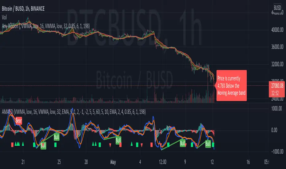
Any RibbonThis indicator displays a ribbon of two individually configured Fast and Slow and Moving Averages for a fixed time frame. It also displays the last close price of the configured time frame, colored green when above the band, red below and blue when interacting. A label shows the percentage distance of the current price from the band, (again red below, green above, blue interacting), when the price is within the band it will show the percentage distance from median of the band.
The Fast and Slow Moving Averages can be set to:
Simple Moving Average (SMA)
Exponential Moving Average (EMA)
Weighted Moving Average (WMA)
Volume-Weighted Moving Average (VWMA)
Hull Moving Average (HMA)
Exponentially Weighted Moving Average (RMA) (SMMA)
Linear regression curve Moving Average (LSMA)
Double EMA (DEMA)
Double SMA (DSMA)
Double WMA (DWMA)
Double RMA (DRMA)
Triple EMA (TEMA)
Triple SMA (TSMA)
Triple WMA (TWMA)
Triple RMA (TRMA)
Symmetrically Weighted Moving Average (SWMA) ** length does not apply **
Arnaud Legoux Moving Average (ALMA)
Variable Index Dynamic Average (VIDYA)
Fractal Adaptive Moving Average (FRAMA)
I wrote this script after identifying some interesting moving average bands with my AMACD indicator and wanting to see them on the price chart. As an example look at the interactions between ETHBUSD 4hr and the band of VIDYA 32 Open and VIDYA 39 Open. Or start from the good old BTC Bull market support band, Weekly EMA 21 and SMA 20 and see if you can get a better fit. I find the Double RMA 22 a better fast option than the standard EMA 21.

AMACD - All Moving Average Convergence DivergenceThis indicator displays the Moving Average Convergane and Divergence ( MACD ) of individually configured Fast, Slow and Signal Moving Averages. Buy and sell alerts can be set based on moving average crossovers, consecutive convergence/divergence of the moving averages, and directional changes in the histogram moving averages.
The Fast, Slow and Signal Moving Averages can be set to:
Exponential Moving Average ( EMA )
Volume-Weighted Moving Average ( VWMA )
Simple Moving Average ( SMA )
Weighted Moving Average ( WMA )
Hull Moving Average ( HMA )
Exponentially Weighted Moving Average (RMA) ( SMMA )
Symmetrically Weighted Moving Average ( SWMA )
Arnaud Legoux Moving Average ( ALMA )
Double EMA ( DEMA )
Double SMA (DSMA)
Double WMA (DWMA)
Double RMA ( DRMA )
Triple EMA ( TEMA )
Triple SMA (TSMA)
Triple WMA (TWMA)
Triple RMA (TRMA)
Linear regression curve Moving Average ( LSMA )
Variable Index Dynamic Average ( VIDYA )
Fractal Adaptive Moving Average ( FRAMA )
If you have a strategy that can buy based on External Indicators use 'Backtest Signal' which returns a 1 for a Buy and a 2 for a sell.
'Backtest Signal' is plotted to display.none, so change the Style Settings for the chart if you need to see it for testing.
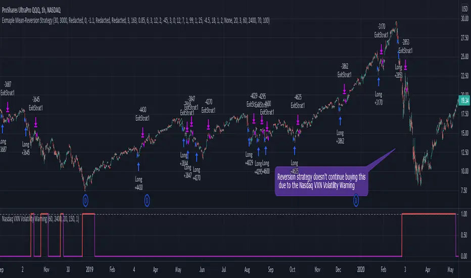
Nasdaq VXN Volatility Warning IndicatorToday I am sharing with the community a volatility indicator that uses the Nasdaq VXN Volatility Index to help you or your algorithms avoid black swan events. This is a similar the indicator I published last week that uses the SP500 VIX, but this indicator uses the Nasdaq VXN and can help inform strategies on the Nasdaq index or Nasdaq derivative instruments.
Variance is most commonly used in statistics to derive standard deviation (with its square root). It does have another practical application, and that is to identify outliers in a sample of data. Variance is defined as the squared difference between a value and its mean. Calculating that squared difference means that the farther away the value is from the mean, the more the variance will grow (exponentially). This exponential difference makes outliers in the variance data more apparent.
Why does this matter?
There are assets or indices that exist in the stock market that might make us adjust our trading strategy if they are behaving in an unusual way. In some instances, we can use variance to identify that behavior and inform our strategy.
Is that really possible?
Let’s look at the relationship between VXN and the Nasdaq100 as an example. If you trade a Nasdaq index with a mean reversion strategy or algorithm, you know that they typically do best in times of volatility . These strategies essentially attempt to “call bottom” on a pullback. Their downside is that sometimes a pullback turns into a regime change, or a black swan event. The other downside is that there is no logical tight stop that actually increases their performance, so when they lose they tend to lose big.
So that begs the question, how might one quantitatively identify if this dip could turn into a regime change or black swan event?
The Nasdaq Volatility Index ( VXN ) uses options data to identify, on a large scale, what investors overall expect the market to do in the near future. The Volatility Index spikes in times of uncertainty and when investors expect the market to go down. However, during a black swan event, historically the VXN has spiked a lot harder. We can use variance here to identify if a spike in the VXN exceeds our threshold for a normal market pullback, and potentially avoid entering trades for a period of time (I.e. maybe we don’t buy that dip).
Does this actually work?
In backtesting, this cut the drawdown of my index reversion strategies in half. It also cuts out some good trades (because high investor fear isn’t always indicative of a regime change or black swan event). But, I’ll happily lose out on some good trades in exchange for half the drawdown. Lets look at some examples of periods of time that trades could have been avoided using this strategy/indicator:
Example 1 – With the Volatility Warning Indicator, the mean reversion strategy could have avoided repeatedly buying this pullback that led to this asset losing over 75% of its value:
Example 2 - June 2018 to June 2019 - With the Volatility Warning Indicator, the drawdown during this period reduces from 22% to 11%, and the overall returns increase from -8% to +3%
How do you use this indicator?
This indicator determines the variance of VXN against a long term mean. If the variance of the VXN spikes over an input threshold, the indicator goes up. The indicator will remain up for a defined period of bars/time after the variance returns below the threshold. I have included default values I’ve found to be significant for a short-term mean-reversion strategy, but your inputs might depend on your risk tolerance and strategy time-horizon. The default values are for 1hr VXN data/charts. It will pull in variance data for the VXN regardless of which chart the indicator is applied to.
Disclaimer: Open-source scripts I publish in the community are largely meant to spark ideas or be used as building blocks for part of a more robust trade management strategy. If you would like to implement a version of any script, I would recommend making significant additions/modifications to the strategy & risk management functions. If you don’t know how to program in Pine, then hire a Pine-coder. We can help!
S&P500 VIX Volatility Warning IndicatorToday I am sharing with the community a volatility indicator that can help you or your algorithms avoid black swan events. Variance is most commonly used in statistics to derive standard deviation (with its square root). It does have another practical application, and that is to identify outliers in a sample of data. Variance in statistics is defined as the squared difference between a value and its mean. Calculating that squared difference means that the farther away the value is from the mean, the more the variance will grow (exponentially). This exponential difference makes outliers in the variance data more apparent.
Why does this matter?
There are assets or indices that exist in the stock market that might make us adjust our trading strategy if they are behaving in an unusual way. In some instances, we can use variance to identify that behavior and inform our strategy.
Is that really possible?
Let’s look at the relationship between VIX and the S&P500 as an example. If you trade an S&P500 index with a mean reversion strategy or algorithm, you know that they typically do best in times of volatility. These strategies essentially attempt to “call bottom” on a pullback. Their downside is that sometimes a pullback turns into a regime change, or a black swan event. The other downside is that there is no logical tight stop that actually increases their performance, so when they lose they tend to lose big.
So that begs the question, how might one quantitatively identify if this dip could turn into a regime change or black swan event?
The CBOE Volatility Index (VIX) uses options data to identify, on a large scale, what investors overall expect the market to do in the near future. The Volatility Index spikes in times of uncertainty and when investors expect the market to go down. However, during a black swan event, the VIX spikes a lot harder. We can use variance here to identify if a spike in the VIX exceeds our threshold for a normal market pullback, and potentially avoid entering trades for a period of time (I.e. maybe we don’t buy that dip).
Does this actually work?
In backtesting, this cut the drawdown of my index reversion strategies in half. It also cuts out some good trades (because high investor fear isn’t always indicative of a regime change or black swan event). But, I’ll happily lose out on some good trades in exchange for half the drawdown. Lets look at some examples of periods of time that trades could have been avoided using this strategy/indicator:
Example 1 – With the Volatility Warning Indicator, the mean reversion strategy could have avoided repeatedly buying this pullback that led to SPXL losing over 75% of its value:
Example 2 - June 2018 to June 2019 - With the Volatility Warning Indicator, the drawdown during this period reduces from 22% to 11%, and the overall returns increase from -8% to +3%
How do you use this indicator?
This indicator determines the variance of the VIX against a long term mean. If the variance of the VIX spikes over an input threshold, the indicator goes up. The indicator will remain up for a defined period of bars/time after the variance returns below the threshold. I have included default values I’ve found to be significant for a short-term mean-reversion strategy, but your inputs might depend on your risk tolerance and strategy time-horizon. The default values are for 1hr VIX data. It will pull in variance data for the VIX regardless of which chart the indicator is applied to.
Disclaimer : Open-source scripts I publish in the community are largely meant to spark ideas or be used as building blocks for part of a more robust trade management strategy. If you would like to implement a version of any script, I would recommend making significant additions/modifications to the strategy & risk management functions. If you don’t know how to program in Pine, then hire a Pine-coder. We can help!

MACD Alert [All MA in one] [Smart Crypto Trade (SCT)]This code is a gift from "Smart Crypto Trade (SCT)" group
MACD indicator contains 3 EMA, I think one of the best usage of MACD is trend detection and divergences.
In our indicator, you can select the type of Moving averages that used in macd.
You can using "MACD" based on several types of moving averages including:
Exponential Moving Average ( EMA )
Volume-Weighted Moving Average ( VWMA )
Simple Moving Average ( SMA )
Weighted Moving Average ( WMA )
Exponentially Weighted Moving Average (RMA) that used in RSI
Smoothed Moving Average ( SMMA )
Arnaud Legoux Moving Average ( ALMA )
Double EMA ( DEMA )
Double SMA (DSMA)
Double WMA (DWMA)
Double RMA (DRMA)
Triple EMA ( TEMA )
Triple SMA (TSMA)
Triple WMA (TWMA)
Triple RMA (TRMA)
Linear regression curve Moving Average ( LSMA )
Variable Index Dynamic Average ( VIDYA )
Fractal Adaptive Moving Average ( FRAMA )
In other words we tried to collect all the most popular MAs in our MACD indicator.
In addition, you can use four types of alert or alarm conditions for detection LONG or SHORT positions and trends. For this, you must set an alert in alert tab and set the condition based on four defaults conditions.
Enjoy

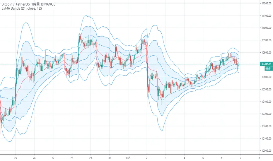
EvMA BandsIt is an index that looks like the final evolution by weighting the Bollinger band with exponential smoothing and volume.
The base Line is my EvMA as volume weighted EMA, so it is quite responsive.
The standard deviation is also exponentially smoothed, and the reaction is too good to handle, so it is further smoothed by EMA.
Charts without volume are not weighted with volume as 1.
It seems that the usage in trading is the same as the Bollinger band
ボリンジャーバンドを指数平滑出来高加重し、最終進化したような指標です
中央線は拙作のEvMAで出来高加重EMAなのでかなり反応が良いです
標準偏差も指数平滑出来高加重して反応が良すぎて扱いにくいのでさらにEMAで平滑化しています
出来高の無いチャートは出来高を1として加重しないようにしています
トレードでの使い方はボリンジャーバンドと同じで良いと思われます
Moving Averages Linear CombinatorLinearly combining moving averages can provide relatively interesting results such as a low-lagging moving averages or moving averages able to produce more pertinent crosses with the price.
As a remainder, a linear combination is a mathematical expression that is based on the multiplication of two variables (or terms) with two coefficients (also called scalars when working with vectors) and adding the results, that is:
ax + by
This expression is a linear combination , with x/y as variables and a/b as coefficients. Lot of indicators are made from linear combinations of moving averages, some examples include the double/triple exponential moving average, least squares moving average and the hull moving average.
Today proposed indicator allow the user to combine many types of moving averages together in order to get different results, we will introduce each settings of the indicator as well as how they affect the final output.
Explaining The Effects Of Linear Combinations
There are various ways to explain why linear combination can produce low-lagging moving averages, lets take for example the linear combination of a fast SMA of period p/2 and slow simple moving average of period p , the linear combination of these two moving averages is described as follows:
MA = 2SMA(p/2) + -1SMA(p)
Which is equivalent to:
MA = 2SMA(p/2) - SMA(p) = SMA(p/2) + SMA(p/2) - SMA(p)
We can see the above linear combinations consist in adding a bandpass filter to the fast moving average, which of course allow to reduce the lag. It is important to note that lag is reduced when the first moving average term is more reactive than the second moving average term. In case we instead use:
MA = -2SMA(p/2) + 1SMA(p)
we would have a combination between a low-pass and band-reject filter.
The Indicator
The indicator is based on the following linear combination:
Coeff × LeadingMA(length) - (Coeff-1) × LaggingMA(length)
The length setting control both moving averages period, leading control the type of moving average used as leading MA, while lagging control the type of MA used as lagging moving average, in order to get low lag results the leading MA should be more reactive than the lagging MA. Coeff control the coefficients of the linear combination, with higher values of coeff amplifying the effects of the linear combination, negative values of coeff would make a low-lag moving average become a lagging moving average, coeff = 1 return the leading MA, coeff = -1 return the lagging MA. The leading period divisor allow to divide the period of the leading MA by the selected number.
The types of moving average available are: simple, exponentially weighted, triangular, least squares, hull and volume weighted. The lagging MA allow you to select another MA on the chart as input.
length = 100, leading period divisor = 2, coeff = 2, with both MA type = SMA. Using coeff = -2 instead would give:
You can select "Plot leading and lagging" in order to show the leading and lagging MA.
Conclusion
The proposed tool allow the user to create a custom moving averages by making use of linear combination. The script is not that useful when you think about it, and might maybe be one of my worst, as it is relatively impractical, not proud of it, but it still took time to make so i decided to post it anyway.

Reflex & Trendflex█ OVERVIEW
Reflex and Trendflex are zero-lag oscillators that decompose price into independent cycle and trend components using SuperSmoother filtering. These indicators isolate each component separately, providing clearer identification of cyclical reversals (Reflex) versus trending movements (Trendflex).
Based on Dr. John F. Ehlers' "Reflex: A New Zero-Lag Indicator" article (February 2020, TASC), both oscillators use normalized slope deviation analysis to minimize lag while maintaining signal clarity. The SuperSmoother filter removes high-frequency noise, then deviations from linear regression (Reflex) or current value (Trendflex) are measured and normalized by RMS for consistent amplitude across instruments and timeframes.
█ CONCEPTS
SuperSmoother Filter
Both oscillators begin with a two-pole Butterworth low-pass filter that smooths price data without the excessive lag of simple moving averages. The filter uses exponential decay coefficients and cosine modulation based on the cutoff period, providing aggressive smoothing while preserving signal timing.
Reflex: Cycle Component
Reflex isolates cyclical price behavior by measuring deviation from a linear regression line fitted through the SuperSmoother output. For each bar, the filter calculates a linear slope over the lookback period, then sums how much the smoothed price deviates from this trendline. These deviations represent pure cyclical movement - price oscillations around the dominant trend. The result is normalized by RMS (root mean square) to produce consistent amplitude regardless of volatility or timeframe.
Trendflex: Trend Component
Trendflex extracts trending behavior by measuring cumulative deviation from the current SuperSmoother value. Instead of comparing to a regression line, it simply sums the differences between the current smoothed value and all past values in the period. This captures sustained directional movement rather than oscillations. Like Reflex, normalization by RMS ensures comparable readings across different instruments.
RMS Normalization
Both oscillators normalize their raw deviation measurements using an exponentially weighted RMS calculation: `rms = 0.04 * deviation² + 0.96 * rms `. This adaptive normalization ensures the oscillator amplitude remains stable as volatility changes, making threshold levels meaningful across different market conditions.
█ INTERPRETATION
Reflex (Cycle Component)
Oscillates around zero representing cyclical price behavior isolated from trend:
• Above zero : Price is in upward phase of cycle
• Below zero : Price is in downward phase of cycle
• Zero crossings : Potential cycle reversal points
• Extremes : Indicate stretched cyclical condition, often precede mean reversion
Best used for identifying cyclical turning points in ranging or oscillating markets. More sensitive to reversals than Trendflex.
Trendflex (Trend Component)
Oscillates around zero representing trending behavior isolated from cycles:
• Above zero : Sustained upward trend
• Below zero : Sustained downward trend
• Zero crossings : Trend direction changes
• Magnitude : Strength of trend (larger absolute values = stronger trend)
Best used for confirming trend direction and identifying trend exhaustion. Less noisy than Reflex due to focus on directional movement rather than oscillations.
Combined Analysis
Using both oscillators together provides powerful signal confirmation:
• Both positive: Strong uptrend with positive cycle phase (high probability long setup)
• Both negative: Strong downtrend with negative cycle phase (high probability short setup)
• Divergent signals: Conflicting cycle and trend (choppy conditions, reduce position size)
• Reflex reversal with Trendflex agreement: Cyclical turn within established trend (entry/exit timing)
Dynamic Thresholds
Threshold bands identify statistically significant oscillator readings that warrant attention:
• Breach above +threshold : Strong bullish cycle (Reflex) or trend (Trendflex) behavior - potential overbought condition
• Breach below -threshold : Strong bearish cycle or trend behavior - potential oversold condition
• Return inside thresholds : Signal strength normalizing, potential reversal or consolidation ahead
• Threshold compression : During low volatility, thresholds narrow (especially with StdDev mode), making breaches more frequent
• Threshold expansion : During high volatility, thresholds widen, filtering out minor oscillations
Combine threshold breaches with zero-line position for stronger signals:
• Threshold breach + zero-line cross = high-conviction signal
• Threshold breach without zero-line support = monitor for confirmation
Alert Conditions
Six built-in alerts trigger on bar close (no repainting):
• Above +Threshold : Oscillator crossed above positive threshold (strong bullish behavior)
• Below -Threshold : Oscillator crossed below negative threshold (strong bearish behavior)
• Reflex Above Zero : Reflex crossed above zero (bullish cycle phase)
• Reflex Below Zero : Reflex crossed below zero (bearish cycle phase)
• Trendflex Above Zero : Trendflex crossed above zero (bullish trend shift)
• Trendflex Below Zero : Trendflex crossed below zero (bearish trend shift)
█ SETTINGS & PARAMETER TUNING
Oscillator Settings
• Source : Price series to decompose
• Reflex Period (5-50): SuperSmoother period for cycle component. Lower values increase responsiveness to cyclical turns but add noise. Default 20.
• Trendflex Period (5-50): SuperSmoother period for trend component. Lower values respond faster to trend changes. Default 20.
Display Settings
• Reflex/Trendflex Display : Toggle visibility and customize colors for each oscillator independently
• Zero Line : Reference line showing neutral oscillator position
Dynamic Thresholds
Optional significance bands that identify when oscillator readings indicate strong cyclical or trending behavior:
• Threshold Mode : Choose calculation method based on market characteristics
- MAD (Median Absolute Deviation) : Outlier-resistant, best for markets with occasional spikes (default)
- Standard Deviation : Volatility-sensitive, adapts quickly to regime changes
- Percentile Rank : Fixed probability bands (e.g., 90% = only 10% of values exceed threshold)
• Apply To : Select which oscillator (Reflex or Trendflex) to calculate thresholds for
• Period (2-200): Lookback window for threshold calculation. Default 50.
• Multiplier (k) : Scaling factor for MAD/StdDev modes. Higher values = fewer threshold breaches (default 1.5)
• Percentile (%) : For Percentile mode only. Higher percentile = more selective threshold (default 90%)
Parameter Interactions
• Shorter periods make both oscillators more sensitive but noisier
• Reflex typically more volatile than Trendflex at same period settings
• For ranging markets: shorter Reflex period (10-15) captures swings better
• For trending markets: shorter Trendflex period (10-15) follows trend shifts faster
█ LIMITATIONS
Inherent Characteristics
• Near-zero lag, not zero-lag : Despite the name, some lag remains from SuperSmoother filtering
• Normalization artifacts : RMS normalization can produce unusual readings during volatility regime changes
• Period dependency : Oscillator characteristics change significantly with different period settings - no "correct" universal parameter
Market Conditions to Avoid
• Very low volatility : Normalization amplifies noise in quiet markets, producing false signals
• Sudden gaps : SuperSmoother assumes continuous data; large gaps disrupt filter continuity requiring bars to stabilize
• Micro timeframes : Sub-minute charts contain microstructure noise that overwhelms signal quality
Parameter Selection Pitfalls
• Matching periods to dominant cycle : If period doesn't align with actual market cycle period, signals degrade
• Threshold over-tuning : Optimizing threshold parameters for past data often fails forward - use conservative defaults
• Ignoring component differences : Reflex and Trendflex measure different aspects - don't expect identical behavior
█ NOTES
Credits
These indicators are based on Dr. John F. Ehlers' "Reflex: A New Zero-Lag Indicator" published in the February 2020 issue of Technical Analysis of Stocks & Commodities (TASC) magazine. The article introduces a novel approach to isolating cycle and trend components using SuperSmoother filtering combined with normalized deviation analysis.
For those interested in the underlying mathematics and DSP concepts:
• Ehlers, J.F. (February 2020). "Reflex: A New Zero-Lag Indicator" - Technical Analysis of Stocks & Commodities magazine
• Ehlers, J.F. (2001). Rocket Science for Traders: Digital Signal Processing Applications . John Wiley & Sons
• Various TASC articles by John Ehlers on SuperSmoother filters and oscillator design
by ♚@e2e4

[BTX] TRIX + MA combined indicator (open version)This indicator combines TRIX and MA of TRIX in one. You can choose which type of moving average line to be used (EMA or SMA).
Default values are 12 periods for TRIX and 10 periods for MA/TRIX, which helps better response to price movement.
This indicator can use in all markets, all timeframes. This is an update to my indicator, which is a protected script. You can find it at the link: .
What is the TRIX (Triple Exponential Average) indicator?
TRIX is a momentum oscillator that displays the percent rate of change of a triple exponentially smoothed moving average. It was developed in the early 1980s by Jack Hutson, an editor for 'Technical Analysis of Stocks and Commodities' magazine. With its triple smoothing, TRIX is designed to filter out insignificant price movements. Chartists can use TRIX to generate signals similar to MACD. A signal line can be applied to look for signal line crossovers. A directional bias can be determined with the absolute level. Bullish and bearish divergences can be used to anticipate reversals.

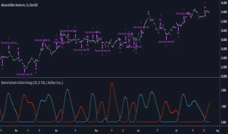
Bilateral Stochastic Oscillator StrategyIntroduction
Strategy based on the bilateral stochastic oscillator, this oscillator aim to detect trends and possible reversal points of the current trend. The oscillator is composed of 1 bull line in blue and 1 bear line in red as well as a signal line in orange, the strategy have many options such as two different strategy framework and a martingale mode. If you require more information about the indicator go check it into my uploaded indicators.
Strategy Frameworks
There are two frameworks available that can be selected from the strategy settings window. Both have the same closing conditions, the "Bull/Bear Cross" entry conditions are :
Buy : when the bull line cross over the bear line
Sell : when the bear line cross over the bull line
The "Signal Cross" entry conditions are :
Buy : when the bull line cross over the signal line
Sell : when the bear line cross over the signal line
Both have the same close conditions that is : close when bull/bear cross under the signal line.
Introduction To Martingale
The martingale money management system consist to double the order size after a loosing trade and can be described as a 2^x where x is the current number of loosing trades since the last win trade, when we win a trade the order size return to the default order size. Therefore our order size function is based on exponential growth.
This system enable the trader to win back his previous losses plus a potential profit, martingales must always be used with stops and sometimes take profits in order to get control in a strategy.
It must always be taken into account that in a series of losses the balance can exponentially decay thus ending to 0 in a matter of trades, this is why it is not recommended to use such system. The strategy allow you to select a martingale multiplier that can be inferior to 2 thus limiting risks, a multiplied of 1 disable the martingale.
Results
Those are the some statistics of the strategy applied to some forex majors by using the default settings in a time frames of 15 minutes.
//-------------------------------------------------------
EURUSD - Order Size 1000 - Spread 0.0002
Profit : $ 21.08
Trades : 19
PP : 57.89 %
Profit Factor : 3.228
Max Drawdown : -$ 3.81
Average Trade : $ 1.11
//-------------------------------------------------------
GBPUSD - Order Size 1000 - Spread 0.0002
Profit : $ 2.31
Trades : 20
PP : 55 %
Profit Factor : 0.938
Max Drawdown : -$ 20.29
Average Trade : $ 0.12
//-------------------------------------------------------
EURAUD - Order Size 1000 - Spread 0.0002
Profit : -$ 9.22
Trades : 20
PP : 40 %
Profit Factor : 0.698
Max Drawdown : -$ 23.44
Average Trade : $ 0.46
//-------------------------------------------------------
EURCHF - Order Size 1000 - Spread 0.0002
Profit : $ 1.58
Trades : 24
PP : 54.17 %
Profit Factor : 1.103
Max Drawdown : -$ 7.23
Average Trade : $ 0.07
//-------------------------------------------------------
Conclusions
Based on the results the strategy does not posses the sufficient performance in order to apply a martingale or any other growth systems as order size. Parameters might be subject to drastic changes depending on the market/time-frame in order to return long-term positive results. I let you draw your conclusions.
Tripple Smoothed RSITriple Exponentially Smoothed RSI by Mauritz van der Walt
If you like this idea, find it useful or use it anywhere please inform me @ www.tradingview.com
I use the RSI primarily for divergences and was in need for something more smooth to spot divergences easier without adding too much lag. Therefor I decided to use a Triple Exponential Moving Average (TEMA) to achieve this. /
The settings for all three EMA are exposed. After smoothing I rescale the value between 0 and 100 using the stochastics technique.

lib_kernelLibrary "lib_kernel"
Library "lib_kernel"
This is a tool / library for developers, that contains several common and adapted kernel functions as well as a kernel regression function and enum to easily select and embed a list into the settings dialog.
How to Choose and Modify Kernels in Practice
Compact Support Kernels (e.g., Epanechnikov, Triangular): Use for localized smoothing and emphasizing nearby data.
Oscillatory Kernels (e.g., Wave, Cosine): Ideal for detecting periodic patterns or mean-reverting behavior.
Smooth Tapering Kernels (e.g., Gaussian, Logistic): Use for smoothing long-term trends or identifying global price behavior.
kernel_Epanechnikov(u)
Parameters:
u (float)
kernel_Epanechnikov_alt(u, sensitivity)
Parameters:
u (float)
sensitivity (float)
kernel_Triangular(u)
Parameters:
u (float)
kernel_Triangular_alt(u, sensitivity)
Parameters:
u (float)
sensitivity (float)
kernel_Rectangular(u)
Parameters:
u (float)
kernel_Uniform(u)
Parameters:
u (float)
kernel_Uniform_alt(u, sensitivity)
Parameters:
u (float)
sensitivity (float)
kernel_Logistic(u)
Parameters:
u (float)
kernel_Logistic_alt(u)
Parameters:
u (float)
kernel_Logistic_alt2(u, sigmoid_steepness)
Parameters:
u (float)
sigmoid_steepness (float)
kernel_Gaussian(u)
Parameters:
u (float)
kernel_Gaussian_alt(u, sensitivity)
Parameters:
u (float)
sensitivity (float)
kernel_Silverman(u)
Parameters:
u (float)
kernel_Quartic(u)
Parameters:
u (float)
kernel_Quartic_alt(u, sensitivity)
Parameters:
u (float)
sensitivity (float)
kernel_Biweight(u)
Parameters:
u (float)
kernel_Triweight(u)
Parameters:
u (float)
kernel_Sinc(u)
Parameters:
u (float)
kernel_Wave(u)
Parameters:
u (float)
kernel_Wave_alt(u)
Parameters:
u (float)
kernel_Cosine(u)
Parameters:
u (float)
kernel_Cosine_alt(u, sensitivity)
Parameters:
u (float)
sensitivity (float)
kernel(u, select, alt_modificator)
wrapper for all standard kernel functions, see enum Kernel comments and function descriptions for usage szenarios and parameters
Parameters:
u (float)
select (series Kernel)
alt_modificator (float)
kernel_regression(src, bandwidth, kernel, exponential_distance, alt_modificator)
wrapper for kernel regression with all standard kernel functions, see enum Kernel comments for usage szenarios. performance optimized version using fixed bandwidth and target
Parameters:
src (float) : input data series
bandwidth (simple int) : sample window of nearest neighbours for the kernel to process
kernel (simple Kernel) : type of Kernel to use for processing, see Kernel enum or respective functions for more details
exponential_distance (simple bool) : if true this puts more emphasis on local / more recent values
alt_modificator (float) : see kernel functions for parameter descriptions. Mostly used to pronounce emphasis on local values or introduce a decay/dampening to the kernel output

Daily Play Ace SpectrumSo the idea of the Daily Play Ace Spectrum is to extend the Ace Spectrum .
By exposing more parameters, making a variation of the Ace Spectrum which is more configurable.
The idea is this makes the Daily Play Ace Spectrum more suitable for use on shorter (hourly and minute) time scales.
These specific parameters exposed still maintain the original form of the original Ace Spectrum, but loosen up the hard coded assumptions of the original indicator.
By exposing more parameters this now makes the Daily Ace Spectrum more sensitive to input.
Meaning the parameters you choose are important and will set the characteristic reaction of the indicator to the series you give it.
This presents a trade-off, the simplicity of the original indicator is sacrificed.
But what's gained is a more comprehensive indicator that now needs more careful parameter adjustment .
Related to the Ace Spectrum:

Volume Flow Anatomy [Kodexius]Volume Flow Anatomy is a dynamic, multi-dimensional volume map that reconstructs how buy, sell, and “stealth” activity is distributed across price rather than just across time. Instead of relying on a static, session-based volume profile, it uses an exponentially decaying memory of recent bars to build a constantly evolving “anatomy” of the auction, where each price level carries an adaptive history of order flow.
The script separates buy vs. sell pressure, adds a third “Stealth Flow” dimension for low-volume price movement (ease of movement / divergence), and automatically derives POC, Value Area, imbalances, absorption zones, and classic profile shapes (D, P, b, B). This gives the trader a compact but highly information-dense map on the right side of the chart to read control (buyers vs. sellers), structure (balanced vs. trending vs. double distribution), and key reaction levels (support/resistance born from flow, not just wicks).
🔹 Features
🔸 Dynamic Lookback with Decay
- The script computes an effective lookback N from the Decay Factor and caps it with Max Lookback.
- Higher decay keeps more history; lower decay emphasizes the most recent flow.
- The profile continuously adapts as new bars are printed.
🔸 Price-Bucketed Flow Map
Each bucket accumulates:
- Sell Flow (sell pressure)
- Buy Flow (buy pressure)
- Stealth Flow (low-volume price movement)
- Box width at each bucket is proportional to the relative intensity of that component.
🔸 Stealth Flow (Low-Volume Price Movement)
- Measures close to close movement relative to volume, emphasizing price movement that occurs on comparatively low volume.
- Helps reveal hidden participation, inefficient moves, and areas that may be vulnerable to re-tests or reversions.
🔸 POC & 70% Value Area (VA)
- Identifies the Point of Control (price bucket with the highest total volume) over the effective lookback.
- Builds a 70% Value Area by expanding from POC towards the nearest high volume neighbors until 70% of the total volume is included.
- POC is drawn as a line over the analyzed range; VA is displayed as a shaded band in the profile area.
🔸 Market Profile Shape Detection
Splits the profile vertically into three zones (bottom / middle / top) and compares their volume distribution.
Classifies structure as:
- D-Shape (Balanced)
- P-Shape (Short Covering)
- b-Shape (Long Liquidation)
- B-Shape (Double Distribution)
Displays a shape label with color coded bias for quick auction context interpretation.
🔸 Imbalance Zones & Absorption
Imbalance: detects buckets where Buy Flow or Sell Flow exceeds the opposite side by at least Imbalance Ratio.
Absorption: flags zones with high volume but low price “ease”, where price is not moving much despite significant volume.
Extends these levels into horizontal zones, marking potential support/resistance and trap areas.
Bullish Imbalance Zone :
Bearish Imbalance Zone :
Absorption Zone :
🔸 Range Context & On-Chart Legend
Draws a Range Box covering the dynamically determined lookback (N bars), with a label displaying the effective bar count.
A bottom-right legend summarizes:
- Color keys for Buy / Sell / Stealth
- POC / VA status
- Bullish vs. Bearish dominance percentage
- Profile shape classification
- Imbalance and Absorption conventions
🔹 Calculations
1. Dynamic Lookback & Price Buckets
int N = math.min(int(4 / (1 - decayFactor) - 1), maxHistory)
float priceHigh = ta.highest(high, N)
float priceLow = ta.lowest(low, N)
float bucketSize = (priceHigh - priceLow) / bucketCount
The effective lookback N is derived from the Decay Factor, using the approximation 4 / (1 - decay) to capture roughly 99% of the decayed influence, then capped with maxHistory to control performance. Over that adaptive range, the script finds the highest and lowest prices and divides the band into bucketCount equal slices (bucketSize). Each slice is a price bucket that will accumulate volume-flow information.
2. Exponentially Decayed Volume Allocation
addValue(array profile, float weight, float minPrice, float maxPrice) =>
for j = 0 to bucketCount - 1
float bucketMin = priceLow + j * bucketSize
float bucketMax = bucketMin + bucketSize
float overlapMin = math.max(minPrice, bucketMin)
float overlapMax = math.min(maxPrice, bucketMax)
float overlapRange = overlapMax - overlapMin
if overlapRange > 0
profile.set(j, profile.get(j) * decayFactor + weight * overlapRange)
This function is the core engine of the indicator. For a given price span and intensity, it checks every bucket for overlap, distributes the weight proportionally to the overlapping range, and before adding new value, decays the existing bucket content by decayFactor. This results in an exponentially weighted profile: recent activity dominates, while older levels retain a gradually fading footprint.
3. POC and 70% Value Area
array totalProfile = array.new(bucketCount, 0)
for j = 0 to bucketCount - 1
float total = sellProfile.get(j) + buyProfile.get(j)
totalProfile.set(j, total)
if total > eaMax
eaMax := total
int pocIdx = 0
float pocVal = 0.0
for j = 0 to bucketCount - 1
if totalProfile.get(j) > pocVal
pocVal := totalProfile.get(j)
pocIdx := j
float totalSum = totalProfile.sum()
float targetSum = totalSum * 0.70
int vaLow = pocIdx
int vaHigh = pocIdx
float currentSum = pocVal
while currentSum < targetSum and (vaLow > 0 or vaHigh < bucketCount - 1)
float lowVal = vaLow > 0 ? totalProfile.get(vaLow - 1) : 0.0
float highVal = vaHigh < bucketCount - 1 ? totalProfile.get(vaHigh + 1) : 0.0
First, totalProfile is built as the sum of buy and sell flow per bucket, and eaMax (the maximum total) is tracked for later normalization. The POC bucket (pocIdx) is simply the index with the highest totalProfile value.
To compute the 70% Value Area, the algorithm starts at the POC bucket and expands outward, each step adding either the upper or lower neighbor depending on which has more volume. This continues until the cumulative volume reaches 70% of totalSum. The result is a volume-driven VA, not necessarily symmetric around POC, which more accurately represents where the market has truly traded.
4. Market Profile Shape Classification
float volTopThird = 0.0
float volMidThird = 0.0
float volBotThird = 0.0
int thirdIdx = int(bucketCount / 3)
for j = 0 to bucketCount - 1
float val = totalProfile.get(j)
if j < thirdIdx
volBotThird += val
else if j < thirdIdx * 2
volMidThird += val
else
volTopThird += val
float totalVolShape = totalProfile.sum()
string shapeStr = "D-Shape (Balanced)"
if (volTopThird > totalVolShape * 0.20) and (volBotThird > totalVolShape * 0.20) and (volMidThird < totalVolShape * 0.50)
shapeStr := "B-Shape (Double Dist)"
else
if pocIdx > bucketCount * 0.5 and volTopThird > volBotThird * 1.3
shapeStr := "P-Shape (Short Covering)"
else if pocIdx < bucketCount * 0.5 and volBotThird > volTopThird * 1.3
shapeStr := "b-Shape (Long Liquidation)"
else
shapeStr := "D-Shape (Balanced)"
The profile is split into bottom, middle, and top thirds. The script compares how much volume is concentrated in each and combines that with the relative location of POC. If both extremes are heavy and the middle light, it labels a B-Shape (double distribution). If the POC is high and the top dominates the bottom, it’s a P-Shape (short covering). If the POC is low and the bottom dominates, it’s a b-Shape (long liquidation). Otherwise, it defaults to a D-Shape (balanced). This provides a quick, at-a-glance assessment of auction structure.
5. Imbalances, Absorption & Zones
bool isBuyImb = showImb and sVal > 0 and (bVal / sVal >= imbRatio)
bool isSellImb = showImb and bVal > 0 and (sVal / bVal >= imbRatio)
float volRatio = eaMax > 0 ? tVal / eaMax : 0
float stRatio = esmRange > 0 ? (stVal - esmMin) / esmRange : 1.0
bool isAbsorp = showAbsorp and volRatio > 0.6 and stRatio < 0.25
if showImbZone
if isSellImb
zoneBoxes.push(box.new(bar_index - N + 1, bucketHi, bar_index + 1, bucketLo, ...))
if isBuyImb
zoneBoxes.push(box.new(bar_index - N + 1, bucketHi, bar_index + 1, bucketLo, ...))
if isAbsorp
zoneBoxes.push(box.new(bar_index - N + 1, bucketHi, bar_index + 1, bucketLo, ...))
Imbalances are identified where one side’s volume (buy or sell) exceeds the other by at least Imbalance Ratio. These buckets are marked as buy or sell imbalance zones, indicating aggressive participation from one side.
Absorption is detected by combining a high volume ratio (volRatio) with a low normalized stealth ratio (stRatio). High volume with limited price movement suggests that opposing orders are absorbing flow at that level. Both imbalance and absorption buckets are extended into horizontal zones from the start of the lookback to the current bar, visually emphasizing key support/resistance and liquidity areas.
6. Building Buy, Sell & Stealth Profiles
sellProfile := array.new(bucketCount, 0)
buyProfile := array.new(bucketCount, 0)
stealthProfile := array.new(bucketCount, 0)
Three arrays are used to store Sell Flow, Buy Flow, and Stealth Flow. Bars are processed from oldest to newest so that decay is applied in correct chronological order. For each bar, a volume density (volume / range) is calculated and distributed across the candle range. Bull candles feed buyProfile, bear candles feed sellProfile.
Stealth Flow computes the close-to-close move between consecutive bars, scaled by 1 / (1 + volume). Big moves on low volume produce high stealth values, which are then allocated across the move’s price span into stealthProfile. This yields a three-layer profile per price level: directional volume and stealthy price movement.

statsLibrary "stats"
stats
factorial(x)
factorial
Parameters:
x (int)
standardize(x, length, lengthSmooth)
standardize
@description Moving Standardization of a time series.
Parameters:
x (float)
length (int)
lengthSmooth (int)
dnorm(x, mean, sd)
dnorm
@description Approximation for Normal Density Function.
Parameters:
x (float)
mean (float)
sd (float)
pnorm(x, mean, sd, log)
pnorm
@description Approximation for Normal Cumulative Distribution Function.
Parameters:
x (float)
mean (float)
sd (float)
log (bool)
ewma(x, length, tau_hl)
ewma
@description Exponentially Weighted Moving Average.
Parameters:
x (float)
length (int)
tau_hl (float)
ewm_sd(x, length, tau_hl)
Exponentially Weighted Moving Standard Deviation.
Parameters:
x (float)
length (int)
tau_hl (float)
ewm_scoring(x, length, tau_hl)
ewm_scoring
@description Exponentially Weighted Moving Standardization:
Parameters:
x (float)
length (int)
tau_hl (float)
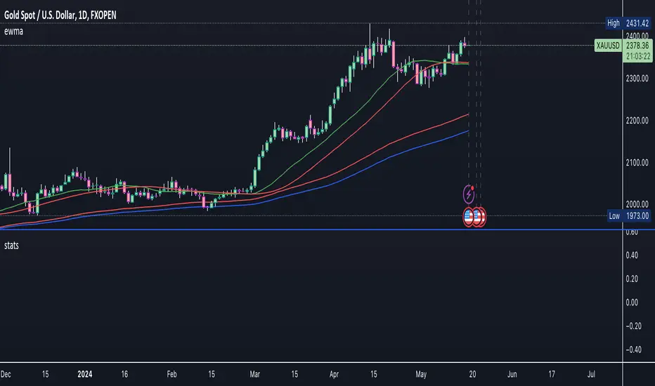
Kaufman Efficiency Ratio-Based Risk PercentageOVERVIEW
The Kaufman Efficiency Ratio-Based Exposure Management indicator uses the Kaufman Efficiency Ratio (KER) to calculate how much you should risk per trade.
If KER is high, then the indicator will tell you to risk more per trade.
A high KER value indicates a trending market, so if you are a trend trader, it makes sense to risk more during these times.
If KER is low, then the indicator will tell you to risk less per trade.
A low KER value indicates a trending market, so if you are a trend trader, it makes sense to risk less during these times.
CONCEPTS
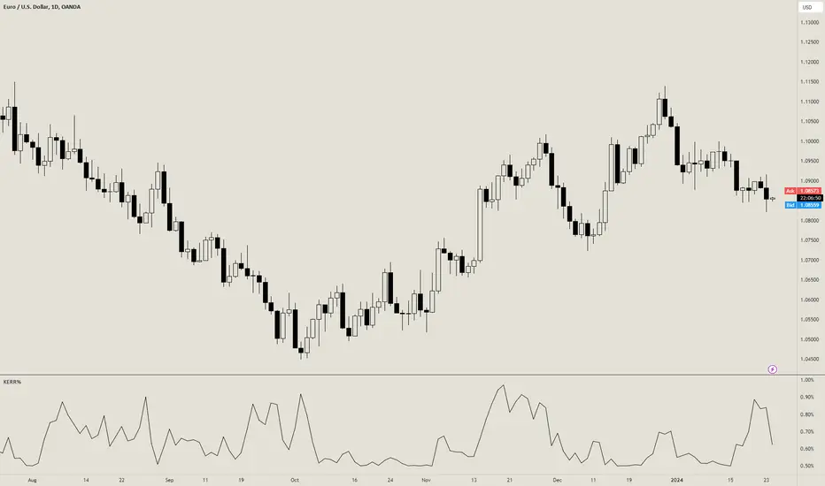
The Kaufman Efficiency Ratio (also known as the Efficiency Ratio, KER, or ER) is a separate indicator developed by Perry J. Kaufman and first published in Kaufman's book, "New Trading Systems and Methods" in 1987.
The KER used to measure the efficiency of a financial instrument's price movement. It is calculated as follows:
KER = (change in price over x bars) / (sum of absolute price changes over x bars)
The first part of the formula, "change in price over x bars" measures the difference between the current close price and the close price x bars ago. The second part of the formula "sum of absolute price changes over x bars" measures the sum of the |open-close| range of each bar between now and x bars ago.
If there is a high change in price over x bars relative to the sum of absolute price changes over x bars, a trending/volatile market is likely in place.
If there is a low change in price over x bars relative to the sum of absolute price changes over x bars, a ranging/choppy market is likely in place.
If you are a trend trader, you can assume that entries taken during high KER periods are more likely to lead to a trend. This indicator helps capitalize on that assumption by increasing risk % per trade during high KER periods, and decreasing risk % per trade during low KER periods.
It uses the following formulas to calculate a KER-adjusted risk % per trade:
Linearly-increasing risk % = min risk + (KER * (max risk - min risk))
Exponentially-increasing risk % = min risk + ((KER^n) * (max risk - min risk))
min risk = the smallest amount you'd be willing to risk on a trade
max risk = the largest amount you'd be willing to risk on a trade
KER = the current Kaufman Efficiency Ratio value
n = an exponent factor used to control the rate of increase of the risk %
Here is an example of how these formulas work:
Assuming that min risk is 0.5%, max risk is 2%, and KER is 0.8 (indicating a trending market), we can calculate the following risk per trade amounts:
Linearly-increasing risk % = 0.5 + (0.8 * (2 - 0.5)) = 1.7%
Exponentially-increasing risk % = 0.5 + ((0.8^3) * (2 - 0.5)) = 1.27%
Now, lets do the same calculations with a lower KER of 0.2 , which indicates a choppy market:
Linearly-increasing risk % = 0.5 + (0.2 * (2 - 0.5)) = 0.8%
Exponentially-increasing risk % = 0.5 + ((0.2^3) * (2 - 0.5)) = 0.51%
With a high KER, we risk more per trade to capitalize on the higher chance of a trending market. With a lower KER, we risk less per trade to protect ourselves from the higher chance of a choppy market.
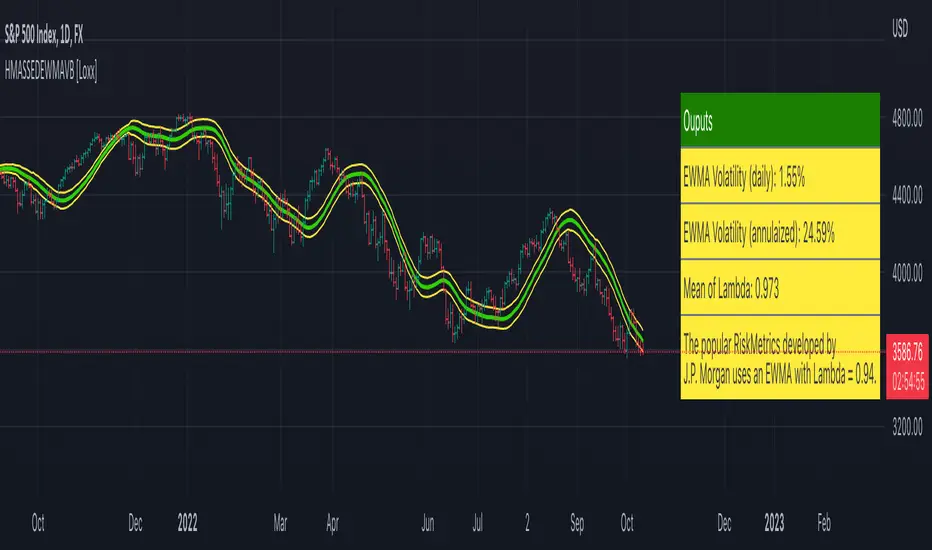
HMA w/ SSE-Dynamic EWMA Volatility Bands [Loxx]This indicator is for educational purposes to lay the groundwork for future closed/open source indicators. Some of thee future indicators will employ parameter estimation methods described below, others will require complex solvers such as the Nelder-Mead algorithm on log likelihood estimations to derive optimal parameter values for omega, gamma, alpha, and beta for GARCH(1,1) MLE and other volatility metrics. For our purposes here, we estimate the rolling lambda (λ) value used to calculate EWMA by minimizing of the sum of the squared errors minus the long-run variance--a rolling window of the one year mean of squared log-returns. In practice, practitioners will use a λ equal to a standardized value put out by institutions such as JP Morgan. Even simpler than this, others use a ratio of (per - 1) / (per + 1) to derive λ where per is the lookback period for EWMA. Due to computation limits in Pine, we'll likely not see a true GARCH(1,1) MLE on Pine for quite some time, but future closed source indicators will contain some very interesting industry hacks to get close by employing modifications to EWMA. Enjoy!
Exponentially weighted volatility and its relationship to GARCH(1,1)
Exponentially weighted volatility--also called exponentially weighted moving average volatility (EWMA)--puts more weight on more recent observations. EWMA is calculated as follows:
σ*2 = λσ(n - 1)^2 + (1 − λ)u(n - 1)^2
The estimate, σn, of the volatility for day n (made at the end of day n − 1) is calculated from σn −1 (the estimate that was made at the end of day n − 2 of the volatility for day n − 1) and u^n−1 (the most recent daily percentage change).
The EWMA approach has the attractive feature that the data storage requirements are modest. At any given time, we need to remember only the current estimate of the variance rate and the most recent observation on the value of the market variable. When we get a new observation on the value of the market variable, we calculate a new daily percentage change to update our estimate of the variance rate. The old estimate of the variance rate and the old value of the market variable can then be discarded.
The EWMA approach is designed to track changes in the volatility. Suppose there is a big move in the market variable on day n − 1 so that u2n−1 is large. This causes our estimate of the current volatility to move upward. The value of λ governs how responsive the estimate of the daily volatility is to the most recent daily percentage change. A low value of λ leads to a great deal of weight being given to the u(n−1)^2 when σn is calculated. In this case, the estimates produced for the volatility on successive days are themselves highly volatile. A high value of λ (i.e., a value close to 1.0) produces estimates of the daily volatility that respond relatively slowly to new information provided by the daily percentage change.
The RiskMetrics database, which was originally created by JPMorgan and made publicly available in 1994, used the EWMA model with λ = 0.94 for updating daily volatility estimates. The company found that, across a range of different market variables, this value of λ gives forecasts of the variance rate that come closest to the realized variance rate. In 2006, RiskMetrics switched to using a long memory model. This is a model where the weights assigned to the u(n -i)^2 as i increases decline less fast than in EWMA.
GARCH(1,1) Model
The EWMA model is a particular case of GARCH(1,1) where γ = 0, α = 1 − λ, and β = λ. The “(1,1)” in GARCH(1,1) indicates that σ^2 is based on the most recent observation of u^2 and the most recent estimate of the variance rate. The more general GARCH(p, q) model calculates σ^2 from the most recent p observations on u2 and the most recent q estimates of the variance rate.7 GARCH(1,1) is by far the most popular of the GARCH models. Setting ω = γVL, the GARCH(1,1) model can also be written:
σ(n)^2 = ω + αu(n-1)^2 + βσ(n-1)^2
What this indicator does
Calculate log returns log(close/close(1))
Calculates Lambda (λ) dynamically by minimizing the sum of squared errors. I've restricted this to the daily timeframe so as to not bloat the code with additional logic required to derive an annualized EWMA historical volatility metric.
After the Lambda is derived, EWMA is calculated one last time and the result is the daily volatility
This daily volatility is multiplied by the source and the multiplier +/- the HMA to create the volatility bands
Finally, daily volatility is multiplied by the square-root of days per year to derive annualized volatility. Years are trading days for the asset, for most everything but crypto, its 252, for crypto is 365.
SwiftEdge ApexThis open-source indicator is designed to help traders visually identify aggressive volume activity ("big trades"), place it in the context of dynamic price deviation from an exponentially weighted VWAP, track a developing Point of Control (POC) during a user-defined session, and highlight potential absorption or exhaustion patterns.
Core Components and Original Integration:
Adaptive VWAP with EWMA Deviation Bands
Instead of a standard cumulative VWAP, the script calculates an exponentially weighted moving average (EWMA) of variance on price-volume data (using a user-adjustable lambda sensitivity). This produces smoother, faster-adapting standard deviation bands (1σ to 3σ) that highlight statistically significant price extensions more responsively than simple moving averages.
Tiered Big Trade Detection (Footprint-Style Bubbles)
Volume is compared against a simple moving average over a user-defined lookback period. Trades exceeding customizable multipliers (1.2× to 8×) and a minimum volume threshold are flagged.
For Premium users, the bubble is plotted at the volume-weighted average price within the bar's 1-second sub-bars (true footprint precision). Non-Premium users fall back to the bar's close price (no errors occur). Bubble size scales with multiplier strength, with white outlines on the largest ones for clarity, and bubbles are colored green/red based on candle direction.
Live Session-Based POC
Volume is accumulated at price levels (rounded to 10 ticks) starting from a configurable session time (default 09:00). The array resets on new sessions or daily changes, producing a developing POC line that acts as a potential value-area magnet or support/resistance reference.
Absorption & Exhaustion Filters
Absorption: High-volume bars with unusually small range (below average range × user multiplier) are marked with lime/red triangles — suggesting hidden buying/selling pressure.
Exhaustion: Extremely high-volume bars with tiny bodies (small close-open relative to range) receive a background tint and "EXH" label — indicating potential climactic activity or fatigue.
How the Elements Work Together:
The VWAP bands provide overall market context (is price extended?). Big-trade bubbles show where aggressive participants are active. The session POC adds a developing fair-value reference. Absorption and exhaustion signals help interpret whether big volume is being met with resistance (absorption → possible continuation) or capitulation (exhaustion → possible reversal). Together they create a layered "smart money footprint" overlay rather than isolated plots.
How to Use the Indicator:
Apply to liquid instruments with reliable volume data (futures, major stocks, large-cap crypto).
In the "Big Trade Bobler" settings:
Adjust lookback period and minimum volume to reduce noise.
Tune multipliers (lower = more signals, higher = stronger but rarer events).
Turn "Use Premium Bubbles" off if you do not have TradingView Premium (script gracefully uses bar close instead of 1-second data).
Set session start hour/minute for POC calculation (e.g., NYSE open at 9:30).
Enable/disable absorption triangles and exhaustion highlights/labels based on preference.
Interpretation tips:
Watch for clusters of large bubbles near VWAP ±2σ/3σ or close to the POC line.
Absorption on trend bars may indicate continuation.
Exhaustion often appears at swing highs/lows and can precede reversals.
Important Limitations:
1-second footprint precision requires TradingView Premium; non-Premium accounts use standard bar close (still functional but less granular).
Volume data quality depends on the symbol and data feed (tick volume is used as proxy on forex/crypto).
This is a discretionary visualization tool — not a mechanical strategy, no entry/exit signals, and no performance backtest is included.
Volume spikes and patterns do not predict future price movement with certainty; always use in combination with your own analysis and proper risk management.

Password Generator by Chervolino [CHE]Enhancing Password Security with Pine Script: A Deep Dive into Brute-Force Attack Prevention
1. Introduction: The Importance of Password Security
Why Password Security Matters:
In today’s digital age, protecting sensitive information through strong passwords is vital. Weak passwords are vulnerable to brute-force attacks, where attackers try every possible character combination until they guess the correct one.
What is Pine Script?
Pine Script is a scripting language developed by TradingView. While mainly used for financial analysis and strategy creation, its versatility allows us to explore other domains, such as password generation and security analysis.
2. Understanding Brute-Force Attacks
What is a Brute-Force Attack?
A brute-force attack systematically tries every possible combination of characters until the correct password is found. The longer and more complex the password, the more secure it is.
Types of Characters in Passwords:
Lowercase Letters (26 characters): Examples include 'a' to 'z'.
Uppercase Letters (26 characters): Examples include 'A' to 'Z'.
Digits (10 characters): Examples include '0' to '9'.
Special Characters: Characters such as '!@#$%^&*' add further complexity to a password.
3. The Role of Password Length in Security
Why Does Password Length Matter?
The number of possible combinations grows exponentially as the length of the password increases.
For example, a password made of only lowercase letters has 26 possible characters. A 7-character password in this case has 26 raised to the power of 7 possible combinations, which equals about 8 billion possibilities.
In comparison, if uppercase letters are included, the possible combinations jump to 52 raised to the power of 7, resulting in over 1 trillion combinations.
Time to Crack a Password:
Assuming a computer can test 2.15 billion passwords per second:
A 7-character password with only lowercase letters can be cracked in about 3.74 seconds.
If uppercase letters are added, it takes approximately 8 minutes.
Adding numbers and special characters makes the cracking time increase further to hours or even days.
4. Password Strength Analysis Using Pine Script
How Pine Script Helps in Password Analysis:
Pine Script can simulate password strength by generating random passwords and calculating how long it would take for a brute-force attack to crack them based on different character combinations and lengths.
We can experiment with using different types of characters (uppercase, lowercase, digits, special characters) and varying the length of the password to estimate the security.
For example:
A password consisting only of lowercase letters would take just a few seconds to crack.
By adding uppercase letters, the time increases to several minutes.
Including digits and special characters can make a password secure for many hours, or even days, depending on the length.
5. Results: Time to Crack Passwords
Here’s a textual summary of how different passwords can be cracked based on their composition and length:
Password with Lowercase Letters Only:
Length: 8 characters
Time to Crack: Less than 1 second.
Password with Uppercase and Lowercase Letters:
Length: 8 characters
Time to Crack: Approximately 24 hours.
Password with Uppercase, Lowercase, and Digits:
Length: 8 characters
Time to Crack: Around 27 minutes.
Password with Uppercase, Lowercase, Digits, and Special Characters:
Length: 12 characters
Time to Crack: Several hundred years.
From these examples, you can see that adding complexity to a password by using a variety of character types and increasing its length exponentially increases the time required to crack it.
6. Best Practices for Password Security
Use a mix of character types: Include lowercase and uppercase letters, digits, and special characters to increase complexity.
Increase the password length: The longer the password, the more difficult it is to crack.
Avoid predictable patterns: Refrain from using common words, dates, or sequential characters like "123456" or "password123".
Use a password manager: Tools like 1Password or LastPass can help store and manage complex passwords securely, so you only need to remember one master password.
7. Conclusion
Password length and complexity are the two most important factors in protecting against brute-force attacks.
Pine Script offers a powerful way to simulate password generation and security analysis, giving you insights into how secure your password is and how long it would take to crack it.
By applying these techniques, you can ensure that your passwords are strong and secure, making brute-force attacks infeasible.
