FlowStateTrader FlowState Trader - Advanced Time-Filtered Strategy
## Overview
FlowState Trader is a sophisticated algorithmic trading strategy that combines precision entry signals with intelligent time-based filtering and adaptive risk management. Built for traders seeking to achieve their optimal performance state, FlowState identifies high-probability trading opportunities within user-defined time windows while employing dynamic trailing stops and partial position management.
## Core Strategy Philosophy
FlowState Trader operates on the principle that peak trading performance occurs when three elements align: **Focus** (precise entry signals), **Flow** (optimal time windows), and **State** (intelligent position management). This strategy excels at finding reversal opportunities at key support and resistance levels while filtering out suboptimal trading periods to keep traders in their optimal flow state.
## Key Features
### 🎯 Focus Entry System
**Support/Resistance Zone Trading**:
- Dynamic identification of key price levels using configurable lookback periods
- Entry signals triggered when price interacts with these critical zones
- Volume confirmation ensures genuine breakout/reversal momentum
- Trend filter alignment prevents counter-trend disasters
**Entry Conditions**:
- **Long Signals**: Price closes above support buffer, touches support level, with above-average volume
- **Short Signals**: Price closes below resistance buffer, touches resistance level, with above-average volume
- Optional trend filter using EMA or SMA for directional bias confirmation
### ⏰ FlowState Time Filtering System
**Comprehensive Time Controls**:
- **12-Hour Format Trading Windows**: User-friendly AM/PM time selection
- **Multi-Timezone Support**: UTC, EST, PST, CST with automatic conversion
- **Day-of-Week Filtering**: Trade only weekdays, weekends, or both
- **Lunch Hour Avoidance**: Automatically skips low-volume lunch periods (12-1 PM)
- **Visual Time Indicators**: Background coloring shows active/inactive trading periods
**Smart Time Features**:
- Handles overnight trading sessions seamlessly
- Prevents trades during historically poor performance periods
- Customizable trading hours for different market sessions
- Real-time trading window status in dashboard
### 🛡️ Adaptive Risk Management
**Multi-Level Take Profit System**:
- **TP1**: First profit target with optional partial position closure
- **TP2**: Final profit target for remaining position
- **Flexible Scaling**: Choose number of contracts to close at each level
**Dynamic Trailing Stop Technology**:
- **Three Operating Modes**:
- **Conservative**: Earlier activation, tighter trailing (protect profits)
- **Balanced**: Optimal risk/reward balance (recommended)
- **Aggressive**: Later activation, wider trailing (let winners run)
- **ATR-Based Calculations**: Adapts to current market volatility
- **Automatic Activation**: Engages when position reaches profitability threshold
### 📊 Intelligent Position Sizing
**Contract-Based Management**:
- Configurable entry quantity (1-1000 contracts)
- Partial close quantities for profit-taking
- Clear position tracking and P&L monitoring
- Real-time position status updates
### 🎨 Professional Visualization
**Enhanced Chart Elements**:
- **Entry Zone Highlighting**: Clear visual identification of trading opportunities
- **Dynamic Risk/Reward Lines**: Real-time TP and SL levels with price labels
- **Trailing Stop Visualization**: Live tracking of adaptive stop levels
- **Support/Resistance Lines**: Key level identification
- **Time Window Background**: Visual confirmation of active trading periods
**Dual Dashboard System**:
- **Strategy Dashboard**: Real-time position info, settings status, and current levels
- **Performance Scorecard**: Live P&L tracking, win rates, and trade statistics
- **Customizable Sizing**: Small, Medium, or Large display options
### ⚙️ Comprehensive Customization
**Core Strategy Settings**:
- **Lookback Period**: Support/resistance calculation period (5-100 bars)
- **ATR Configuration**: Period and multipliers for stops/targets
- **Reward-to-Risk Ratios**: Customizable profit target calculations
- **Trend Filter Options**: EMA/SMA selection with adjustable periods
**Time Filter Controls**:
- **Trading Hours**: Start/end times in 12-hour format
- **Timezone Selection**: Four major timezone options
- **Day Restrictions**: Weekend-only, weekday-only, or unrestricted
- **Session Management**: Lunch hour avoidance and custom periods
**Risk Management Options**:
- **Trailing Stop Modes**: Conservative/Balanced/Aggressive presets
- **Partial Close Settings**: Enable/disable with custom quantities
- **Alert System**: Comprehensive notifications for all trade events
### 📈 Performance Tracking
**Real-Time Metrics**:
- Net profit/loss calculation
- Win rate percentage
- Profit factor analysis
- Maximum drawdown tracking
- Total trade count and breakdown
- Current position P&L
**Trade Analytics**:
- Winner/loser ratio tracking
- Real-time performance scorecard
- Strategy effectiveness monitoring
- Risk-adjusted return metrics
### 🔔 Alert System
**Comprehensive Notifications**:
- Entry signal alerts with price and quantity
- Take profit level hits (TP1 and TP2)
- Stop loss activations
- Trailing stop engagements
- Position closure notifications
## Strategy Logic Deep Dive
### Entry Signal Generation
The strategy identifies high-probability reversal points by combining multiple confirmation factors:
1. **Price Action**: Looks for price interaction with key support/resistance levels
2. **Volume Confirmation**: Ensures sufficient market interest and liquidity
3. **Trend Alignment**: Optional filter prevents counter-trend positions
4. **Time Validation**: Only trades during user-defined optimal periods
5. **Zone Analysis**: Entry occurs within calculated buffer zones around key levels
### Risk Management Philosophy
FlowState Trader employs a three-tier risk management approach:
1. **Initial Protection**: ATR-based stop losses set at strategy entry
2. **Profit Preservation**: Trailing stops activate once position becomes profitable
3. **Scaled Exit**: Partial profit-taking allows for both security and potential
### Time-Based Edge
The time filtering system recognizes that not all trading hours are equal:
- Avoids low-volume, high-spread periods
- Focuses on optimal liquidity windows
- Prevents trading during news events (lunch hours)
- Allows customization for different market sessions
## Best Practices and Optimization
### Recommended Settings
**For Scalping (1-5 minute charts)**:
- Lookback Period: 10-20
- ATR Period: 14
- Trailing Stop: Conservative mode
- Time Filter: Major session hours only
**For Day Trading (15-60 minute charts)**:
- Lookback Period: 20-30
- ATR Period: 14-21
- Trailing Stop: Balanced mode
- Time Filter: Extended trading hours
**For Swing Trading (4H+ charts)**:
- Lookback Period: 30-50
- ATR Period: 21+
- Trailing Stop: Aggressive mode
- Time Filter: Disabled or very broad
### Market Compatibility
- **Forex**: Excellent for major pairs during active sessions
- **Stocks**: Ideal for liquid stocks during market hours
- **Futures**: Perfect for index and commodity futures
- **Crypto**: Effective on major cryptocurrencies (24/7 capability)
### Risk Considerations
- **Market Conditions**: Performance varies with volatility regimes
- **Timeframe Selection**: Lower timeframes require tighter risk management
- **Position Sizing**: Never risk more than 1-2% of account per trade
- **Backtesting**: Always test on historical data before live implementation
## Educational Value
FlowState serves as an excellent learning tool for:
- Understanding support/resistance trading
- Learning proper time-based filtering
- Mastering trailing stop techniques
- Developing systematic trading approaches
- Risk management best practices
## Disclaimer
This strategy is for educational and informational purposes only. Past performance does not guarantee future results. Trading involves substantial risk of loss and is not suitable for all investors. Users should thoroughly backtest the strategy and understand all risks before live trading. Always use proper position sizing and never risk more than you can afford to lose.
---
*FlowState Trader represents the evolution of systematic trading - combining classical technical analysis with modern risk management and intelligent time filtering to help traders achieve their optimal performance state through systematic, disciplined execution.*
Cari dalam skrip untuk "Futures"

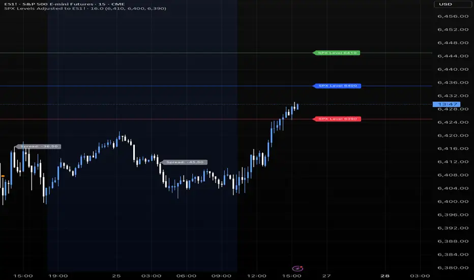
SPX Levels Adjusted to Active TickerThis indicator allows you to plot custom SPX levels directly on the ES1! (E-mini S&P 500 Futures) chart, automatically adjusting for the spread between SPX and ES1!. This is particularly useful for traders who perform technical analysis on SPX but execute trades on ES1!.
Features:
Input up to three SPX key levels to track (e.g., 5000, 4950, 4900)
The script adjusts these levels in real-time based on the current spread between SPX and ES1!
Displays the spread in the chart header for quick reference
Plots updated horizontal lines that move with the spread
Includes optional labels showing the spread periodically to reduce clutter
Supports Multiple Tickers, ES1!, SPY and SPX500USD.
Ideal for futures traders who want SPX context while trading ES1!.

Synthetic VX3! & VX4! continuous /VX futuresTradingView is missing continuous 3rd and 4th month VIX (/VX) futures, so I decided to try to make a synthetic one that emulates what continuous maturity futures would look like. This is useful for backtesting/historical purposes as it enables traders to see how their further out VX contracts would've performed vs the front month contract.
The indicator pulls actual realtime data (if you subscribe to the CBOE data package) or 15 minute delayed data for the VIX spot (the actual non-tradeable VIX index), the continuous front month (VX1!), and the continuous second month (VX2!) continually rolled contracts. Then the indicator's script applies a formula to fairly closely estimate how 3rd and 4th month continuous contracts would've moved.
It uses an exponential mean‑reversion to a long‑run level formula using:
σ(T) = θ+(σ0−θ)e−kT
You can expect it to be off by ~5% or so (in times of backwardation it might be less accurate).

SPX Levels Adjusted to ES1!This indicator allows you to plot custom SPX levels directly on the ES1! (E-mini S&P 500 Futures) chart, automatically adjusting for the spread between SPX and ES1!. This is particularly useful for traders who perform technical analysis on SPX but execute trades on ES1!.
Features:
Input up to three SPX key levels to track (e.g., 5000, 4950, 4900)
The script adjusts these levels in real-time based on the current spread between SPX and ES1!
Displays the spread in the chart header for quick reference
Plots updated horizontal lines that move with the spread
Includes optional labels showing the spread periodically to reduce clutter
Ideal for futures traders who want SPX context while trading ES1!.
Make sure to apply this indicator on the ES1! chart, not SPX.
CME Price Limits (Futures Prop Firm Rule)This indicator shows the CME Price Limit, combined with a safety distance that is used by several futures prop firms. Trading in the highlighted area means a rule violation for many Futures prop firm accounts.
The levels are calculated from the "Settlement as close" closing price of the previous daily candle.

Celestial Pair Spread Hello friends, after a very long time!
Today, I tried to put into code an idea that came to my mind spontaneously and suddenly.
Note :
This script is experimental and improvable.
I haven't had a chance to try it yet.
TIMEFRAME : 1D (Daily Bars)
CELESTIAL SPREAD
The spread moves in a very limited area and is consistent within itself, especially on days far from the end of the contract.
That's why there is a reassuring sky atmosphere. That's why this name was given completely improvised.
Basic logic of the script
We enter the name of the CME Futures contract we want to enter:
Ex : CL1! , ES1! , ZC1! , NQ1!
The script creates us a pair trade parity divided into secondary contracts.
Example : ES1!/ES2!
What is pair trading?
I will explain briefly here.
For users who are wondering:
www.investopedia.com
Let's get back to our topic.
Now we have created a parity that does not actually exist.
This parity is the manifestation of the relative movements of two contracts.
When the parity rises, ES1! increased,ES2! has fallen.
In the opposite case, We can say: ES1! Contract has been dropped ES2! has increased.
Pair trading is generally a trade that needs to be kept in mind from time to time.
It is a method preferred by professionals who can process very quickly.
Market risk is minimal, but since 2 contracts are purchased, more money is paid and very low percentage profits are made.
It is very expensive to do pair trading, especially with oil and its derivatives and interest security derivatives.
The contract we are considering has micros. (small-item contracts tied to the same value)
So when we switch to our broker MES1!/MES2! We will trade.
For all CME futures :
www.cmegroup.com
Anyway, let's continue:
The script created the parity showing its relationship with the next contract and plotted it as bars.
Celestial bands are just like Bollinger bands, but they consist of 3 bands based on percentage changes rather than standard deviation.
The middle band is obtained from moving averages.
The upper and lower bands are the middle band subjected to a threshold value.
The threshold value can be changed.
0.15 percent was charged for this script.
CAUTION :
As can be seen in the example below;
The most important thing is not to make any transactions when the contract switch dates are approaching.
Therefore, it is recommended to use it just below the main chart.
The blue bars in the parity are
Values that outside the upper and lower threshold values are colored blue.
For this condition
Alerts has been added.
Don't forget to add alert and edit.
MAIN PURPOSE
It is aimed to start a pair trade when such conditions come and to quickly close the trades when the parity basis reaches the value.
OTHER IMPORTANT POINTS
Other issues are broker related issues.
Difference between initial margins and maintanence margins of contracts (between 1! and 2!)
It shouldn't be too high.
The commission should not be too high.
Leverage must be high because the profit percentage is very low.
To calculate leverage you must divide your contract size by the relevant margin requirement.
Sample margin requirement table:
www.interactivebrokers.com
RISKS
It is an experimental and intellectual script,
the risk of contract price differences (maybe it will not leave a profit except for very extreme values)
I remind you of the quickness risk that comes from a two-legged trade.
Alerts definitely synchronized with an audible alert sent to a smartphone as an e-mail notification and displayed on the locked screen for quick action.
Best regards!

Position Size Calculator (MOEX Futures)Описание на русском языке
Этот скрипт для TradingView создан специально для трейдеров, работающих с фьючерсами на Московской бирже. Его основная цель – помочь трейдерам быстро и точно рассчитывать параметры позиции, такие как количество контрактов, риск на сделку, общий размер маржи, а также цены стоп-лосса и тейк-профита.
Функционал:
Расчет цены контракта: учитывает цену актива (в пунктах) и стоимость одного пункта.
Риск на сделку: определяется как процент от общего капитала.
Размер позиции: рассчитывается на основе риска на сделку и стоп-лосса.
Количество контрактов: округляется до целого числа вниз.
Общий размер маржи: определяется исходя из количества контрактов и маржи на один контракт.
Цены стоп-лосса и тейк-профита: вычисляются как для лонг-, так и для шорт-позиций.
Интерактивная таблица: статично отображается в правом верхнем углу графика и обновляется автоматически при изменении входных данных.
Скрипт заточен исключительно под специфику фьючерсов Московской биржи и позволяет трейдерам оптимизировать расчёты, минимизировать ошибки и экономить время.
Description in English
This TradingView script is specifically designed for traders working with futures on the Moscow Exchange. Its primary purpose is to help traders quickly and accurately calculate position parameters, such as the number of contracts, risk per trade, total margin size, and stop-loss and take-profit prices.
Features:
Contract price calculation: Takes into account the asset price (in points) and the price per point.
Risk per trade: Defined as a percentage of the total capital.
Position size: Calculated based on the risk per trade and stop-loss percentage.
Number of contracts: Rounded down to the nearest whole number.
Total margin size: Determined based on the number of contracts and margin per contract.
Stop-loss and take-profit prices: Calculated for both long and short positions.
Interactive table: Statically displayed in the top-right corner of the chart and dynamically updated when input parameters change.
This script is tailored exclusively to the specifics of futures trading on the Moscow Exchange, enabling traders to optimize calculations, minimize errors, and save time.

TASC 2023.10 COT Commercials Indicator█ OVERVIEW
This script implements the COT Commercials Indicator introduced by Alfred François Tagher in an article featured in TASC's October 2023 edition of Traders' Tips . The indicator is designed for use in futures markets and represents a fast stochastic (%K) calculated based on the commercial open interest values of an asset derived from the weekly Commitments Of Traders (COT) report .
█ CONCEPTS
The COT report, issued by the Commodity Futures Trading Commission (CFTC) , presents a breakdown of reportable open interest positions held by various trader groups—commercial, noncommercial, and nonreportable (small traders). Open interest reflects the total number of derivative contracts entered by market participants but not yet settled. Consequently, it can serve as a measure of market activity and liquidity.
The indicator showcased here aims to analyze changes in the reported net values of open interest for commercial traders/hedgers (often referred to as 'smart money', as they deal directly in underlying commodities). The net values are positive when the commercial traders have more long positions than short ones and negative when they hold more short positions than long ones. Positive net values indicate that commercial traders hold more long positions than short ones, while negative values indicate the opposite. Thus, overbought and oversold conditions of the COT Commercials Indicator potentially suggest collective bullish and bearish sentiments, respectively.
█ CALCULATIONS
The calculations involve these steps:
1. Net open interest values are extracted from COT data using the LibraryCOT library provided by TradingView.
2. A fast stochastic indicator (%K) is then applied to normalize these net values.
The script also provides an option of calculating and plotting the indicator curve for noncommercial (speculators) open interest.

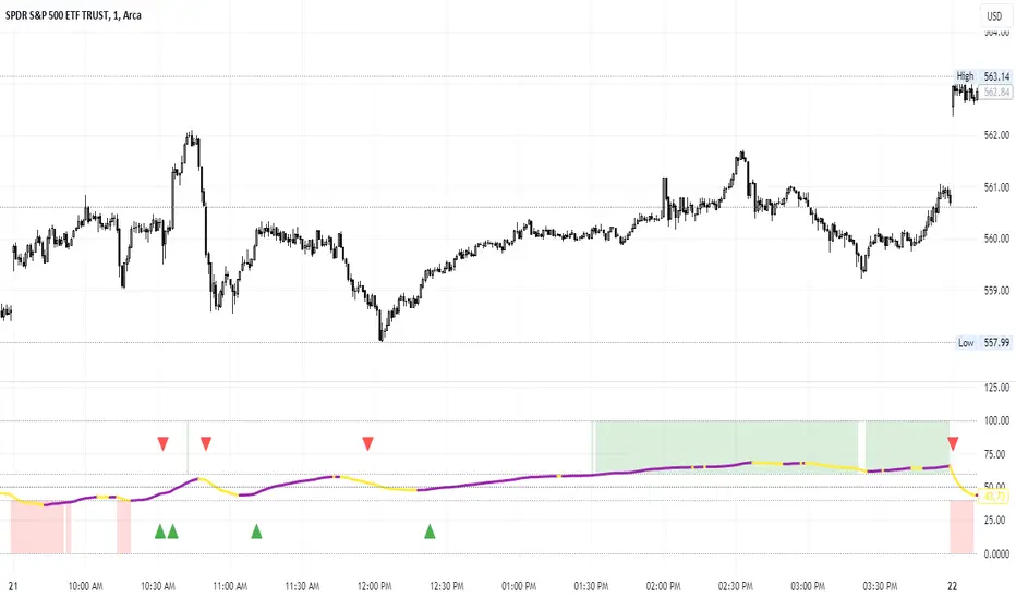
Percent of U.S. Stocks Above VWAPThis indicator plots a line reflecting the percentage of all U.S. stocks above or below their VWAP for the given candle. Horizontal lines have been placed at 40% (oversold), 50% (mid-line), and 60% (overbought). I recommend using this indicator as a market breadth indicator when trading individual stocks. In my experience, this indicator is best utilized while trading the major indices (SPX, SPY, QQQ, IWM) or their futures (ES, NQ, RTY) in the following manner:
- When the line crosses 50%, a green or red triangle is plotted indicating the majority of market momentum has turned bullish or bearish based on price positioning vs. VWAP. Look for longs when the line is rising (green) or above 50%, or shorts when the line is falling (red) or below 50%.
- When the line is below 40%, indicator shows red shading; I would not be long anything during this period. When the line exits this level, I begin looking for long entries. This line is adjustable in the indicator settings if you prefer to use a tighter or looser oversold level.
- When the line is above 60%, indicator shows green shading; I would not be short anything during this period. When the line exits this level, I begin looking for short entries. This line is adjustable in the indicator settings if you prefer to use a tighter or looser overbought level.
This indicator uses the TradingView ticker “PCTABOVEVWAP.US”, thus it only updates during NY market hours. If trading futures, I recommend applying VWAP to your chart and using that as the level to trade against in a similar manner, along with your personal price action analysis and other indicators you find useful.
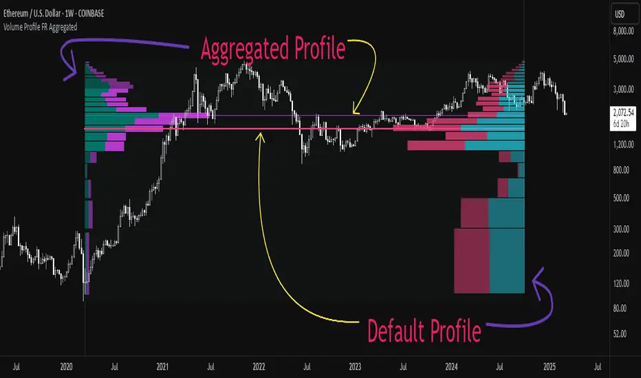
Aggregated Volume Profile Spot & Futures ⚉ OVERVIEW ⚉
Aggregate Volume Profile - Shows the Volume Profile from 9 exchanges. Works on almost all CRYPTO Tickers!
You can enter your own desired exchanges, on/off any others, as well as select the sources of SPOT, FUTURES and others.
The script also includes several input parameters that allow the user to control which exchanges and currencies are included in the aggregated data.
The user can also choose how volume is displayed (in assets, U.S. dollars or euros) and how it is calculated (sum, average, median, or dispersion).
WARNING Indicator is for CRYPTO ONLY.
______________________
⚉ SETTINGS ⚉
‾‾‾‾‾‾‾‾‾‾‾‾‾‾‾‾‾‾‾‾‾‾
Data Type — Choose Single or Aggregated data.
• Single — Show only current Volume.
• Aggregated — Show Aggregated Volume.
Volume By — You can also select how the volume is displayed.
• COIN — Volume in Actives.
• USD — Volume in United Stated Dollar.
• EUR — Volume in European Union.
• RUB — Volume in Russian Ruble.
Calculate By — Choose how Aggregated Volume it is calculated.
• SUM — This displays the total volume from all sources.
• AVG — This displays the average price of the volume from all sources.
• MEDIAN — This displays the median volume from all sources.
• VARIANCE — This displays the variance of the volume from all sources.
• Delta Type — Select the Volume Profile type.
• Bullish — Shows the volume of buyers.
• Bearish — Shows the volume of sellers.
• Both — Shows the total volume of buyers and sellers.
Additional features
The remaining functions are responsible for the visual part of the Volume Profile and are intuitive and I recommend that you familiarize yourself with them simply by using them.
________________
⚉ NOTES ⚉
‾‾‾‾‾‾‾‾‾‾‾‾‾‾‾‾
If you have any ideas what to add to my work to add more sources or make calculations cooler, suggest in DM .
Also I recommend exploring and trying out my similar work.
EuroDollar Curve Implied 3M RateChart shows the Eurodollar futures prices latest prices from Sep 22 onwards. Display logic based on LongFiats code. This needs to be readjusted manually every 3 months whenever the front-month expires. Good tool to see where professional eurodollar futures think interest rates will be over the next few years. Check regularly as sentiment changes.

Binance Big Open Interest Delta Change v2 Note: This script will only work properly with Binance Futures symbols.
This script simply looks at the open interest for the symbol you are currently viewing and determines if a large change in open interest has occurred, which triggers a background color alert.
It does this by comparing the absolute value of the range of the current open interest bar with a simple average (length set by user) of the past x range. The user also determines what is considered a 'large' change in open interest by setting a multiplier with which the current range must exceed compared to the average range in order to trigger an alert.
If the change in open interest is an increase in OI, the alert is blue, and if the change in open interest is a decrease, the alert is orange.
The open interest ticker that is used for calculation is derived by adding the current ticker and "_OI" so that it auto changes each time you switch to a new Binance futures contract.

Liquidations by volume (spot/futures)BINANCE:BTCUSDT
Shows actual liquidations on a per-candle basis by using the difference in volume between spot and futures markets.
i.e. volume on a futures market will be much higher if there are many liquidations.
Long liquidation data should in theory be more accurate than short liquidation data due to the inability to short on a spot market.
This indicator should be able to help identify trends by determining liquidation points in the chart.

SPXL Futures Strategy- Buy/sell signals for SPXL using futures momentum.
- For real-time signals at close, use ES1! on 2 minute chart and sign up for real-time cboe mini futures data feed in tradingview.
- All buys and sells are at near close of US RTH market at 4pm.
- Best to use the script with other breadth signals to decide on trading strategy.
- Script is compatible with SPY, SPXL, RSP, QQQ, TQQQ and many other SPX correlated tickers, however it’s primarily developed for SPX.

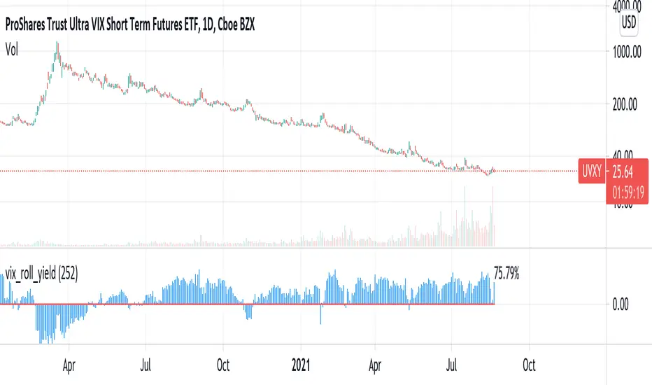
vix_roll_yieldShows the roll yield of the VX futures, which is the ratio of a continuously weighted average of the front two months to the VIX. The VX (VIX futures) contract expires on the third Tuesday of each month. On the next trading day, the front month will have full weighting, and the second month will have no weight. On the expiration day, the back month will have full weighting and the front month will have no weight. In between, the weight gradually shifts.
This weighted average is similar to the SPVIXSTR index that UVXY and several other funds track. When the average is below the VIX, the indicator is negative, and the front month contract will tend to gain value relatively more rapidly than the back month as it converges upward to the VIX spot price. Because funds whose NAV is tied up in VX contracts continuously roll from the (typically cheaper) front month to the back, in situations where the front month is more expensive than usual--or even more expensive than the back month--these products may have a "tailwind". In this case, they are selling expensive front month contracts to purchase cheap back month contracts.
Ordinarily, VIX funds have a "headwind." The roll yield is positive, the front month is cheap, and the back month is expensive. Day by day the funds sell cheap front month contracts and buy expensive back month contracts, which, in turn and over time, become the front month and converge with the VIX, losing value rapidly. This is a brief explanation about the decay of these products.
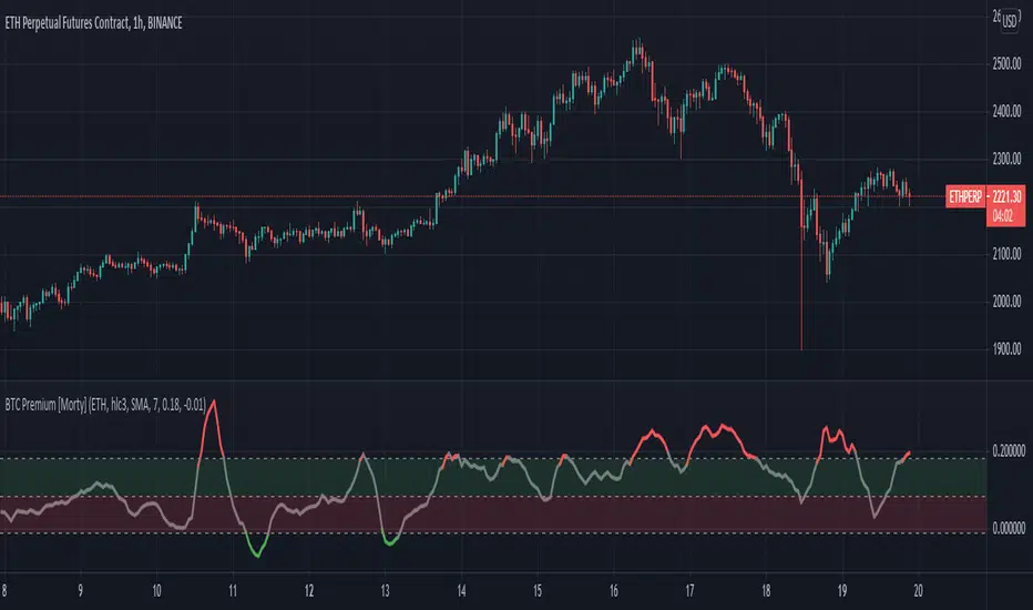
BTC Perpetual Futures Premium [Morty]Version 1.0, 20210409
This is an oscillator indicator that shows the premium between BTC perpetual futures and spot prices.
The prices of futures and spot are weighted average prices, weighted by the exchange's trading volume.
When the indicator is in the upper half of the region, the funding rate of perpetual contracts is relatively high, and the market trend is bullish.
When the indicator is in the upper half of the region, the funding rate of perpetual contracts is relatively high, and the market trend is bearish.
You can set the upper and lower limits of the premium. When the indicator exceeds the upper or lower limit, the trend usually reverses.
Buy the dip, Sell the high.
----------------------------------------------------------
Version 1.0, 20210409
这是一个振荡器指标,它显示了BTC永续期货和现货之间的溢价。
期货和现货的价格是加权平均价格,由交易所的交易量加权。
当指标在上半部区域时,永续合约的资金费率相对较高,市场趋势是牛市。
当指标在上半部区域时,永续合约的资金费率相对较高,市场趋势是熊市。
您可以设置溢价的上限和下限。当指标超过上限或者下限,通常会趋势反转。
Buy the dip, Sell the high.
VIX Near-Term Futures CurveThis indicator provides a 3 day smoothed histogram expressing whether the near term VIX futures curve is in a state of contango or backwardation. The solid red/green bars express the spot vs front-month vs next month curve with the value being the cumulative point spread between them. The shaded overlay bars express the spread between the VIX spot index and front-month futures contract only.
This indicator is to be used on a 1 DAY interval or higher.

ADX Momentum cross + MacD + HH LL + Buy/Sell Signals and alerts Hello, This is the first indicator I have made and would like to contribute to the community.
This strategy came from trying to replicate a previous ADX Cross Indicator that I loved on MT4 which I used successfully on EUR/USD on high and low time frames. Through the process of trying to replicate it I failed, I decided to take what I had written so far and create my own ADX cross strategy using the combination of 3 ADX's, their lag. Then also using Higher highs and lower lows with the MacD to further filter the signals.
There are two buy and two sell conditions , the difference between these are just the order in which the ADX crossing determines the entry. The MacD and higher highs and lower lows are the same for filtering the signal.
You can change the look back for HH and LL look back range, along with the DI Length & ADX Smoothing for all ADX's. The lag used for either the buy or sell strategy with the Lag_Buy/Lag_Sell inputs. Lag_mid setting will affect all 4 conditions.
From testing and based on the ADX cross logic you should follow this structure when changing the inputs for:
DI Length: Lowest DI value (I.E. 1)
DI Lengtha: Middle DI value (I.E. 2)
DI Lengthb: Highest DI value (I.E. 3)
ADX Smoothing: Lowest Smoothing value (I.E. 1)
ADX Smoothinga: Middle Smoothing value (I.E. 2)
ADX Smoothingb: Highest Smoothing value (I.E. 3)
I tested this on the EUR/USD, but mainly I have been using it on BTC/USDT(binance) and BTC/USDT Perpetual futures(binance) with the 5 minute chart. I suggest playing around with the settings depending on the Symbol and timeframe you use because the default settings are what I last found to be optimal for my self on the 5min BTC/USDT Perpetual futures(binance) chart.
A good starting point I found when using the indicator on other charts is to use the below values:
DI Length: 7
DI Lengtha: 14
DI Lengthb: 21
ADX Smoothing: 7
ADX Smoothinga: 14
ADX Smoothingb: 21
If you have any questions, suggestions, or requests for this indicator feel free contact me. You can either comment on here or Message me
If you like this indicator please like and comment where you found it useful.

Open Interest Money Flow Index (OIMFI)CAUTION : This system was inspired from seiglerj' s "Money Flow Index " script. Open Interests are used instead of volume.
What is the Money Flow Index ( MFI )?
The Money Flow Index ( MFI ) is a technical oscillator that uses price and volume for identifying overbought or oversold conditions in an asset. It can also be used to spot divergences which warn of a trend change in price. The oscillator moves between 0 and 100.
Unlike conventional oscillators such as the Relative Strength Index ( RSI ), the Money Flow Index incorporates both price and volume data, as opposed to just price. For this reason, some analysts call MFI the volume-weighted RSI .
What Does the Money Flow Index ( MFI ) Tell You?
One of the primary ways to use the Money Flow Index is when there is a divergence. A divergence is when the oscillator is moving in the opposite direction of price. This is a signal of a potential reversal in the prevailing price trend.
For example, a very high Money Flow Index that begins to fall below a reading of 80 while the underlying security continues to climb is a price reversal signal to the downside. Conversely, a very low MFI reading that climbs above a reading of 20 while the underlying security continues to sell off is a price reversal signal to the upside.
Traders also watch for larger divergences using multiple waves in the price and MFI . For example, a stock peaks at $10, pulls back to $8, and then rallies to $12. The price has made two successive highs, at $10 and $12. If MFI makes a lower higher when the price reaches $12, the indicator is not confirming the new high. This could foreshadow a decline in price.
The overbought and oversold levels are also used to signal possible trading opportunities. Moves below 10 and above 90 are rare. Traders watch for the MFI to move back above 10 to signal a long trade, and to drop below 90 to signal a short trade.
Other moves out of overbought or oversold territory can also be useful. For example, when an asset is in an uptrend, a drop below 20 (or even 30) and then a rally back above it could indicate a pullback is over and the price uptrend is resuming. The same goes for a downtrend. A short-term rally could push the MFI up to 70 or 80, but when it drops back below that could be the time to enter a short trade in preparation for another drop .
Reference : www.investopedia.com
WARNING :
** Since each instrument in the list has its own unique contract data, you must first enter its name to display it. I recommend you to select OANDA from the markets. Finally, when the COT reports are issued, it may repaints. However, this repaint is usually close to closing or after close .(When COT reports are so sharp ) So use this script only 1W ( 1 week ) or 1 M ( 1 month ) timeframe.
** This data is taken to Tradingview with the help of Quandl. This is a very low possibility, but the system will not work if there is a malfunction.
FEATURES :
*** Working with all futures (Including : Bitcoin )
*** If you dont work with "Futures" , you can select "Others" from switchable menu and use volume for all instruments.
*** New generation elegant design used : Adaptive coloring Overbought - Oversold Levels according to the closing price.
NOTE : This code is open source under the MIT License. If you have any improvements or corrections to suggest, please send me a pull request via the github repository github.com
Stay tuned. Best wishes !

BTC South Korea_PricesSince BTC prices are diverging, this set of 4 indicators charts volume-weighted prices for different exchanges:
Spot, Tether, Futures and South Korea.
I tried doing EUR & JPY, but the divergence is minimal so its a little pointless.
Here is the 4 links:

BTC Futures_PricesSince BTC prices are diverging, this set of 4 indicators charts volume-weighted prices for different exchanges:
Spot, Tether, Futures and South Korea.
I tried doing EUR & JPY, but the divergence is minimal so its a little pointless.
Here is the 4 links:

BTC Spot_PricesSince BTC prices are diverging, this set of 4 indicators charts volume-weighted prices for different exchanges:
Spot, Tether, Futures and South Korea.
I tried doing EUR & JPY, but the divergence is minimal so its a little pointless.
Here is the 4 links:
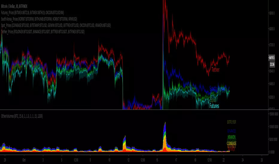
BTC Tether_PricesSince BTC prices are diverging, this set of 4 indicators charts volume-weighted prices for different exchanges:
Spot, Tether, Futures and South Korea.
I tried doing EUR & JPY, but the divergence is minimal so its a little pointless.
Here is the 4 links:
