LYFX-GOLD-15MIndicator Operation Method:
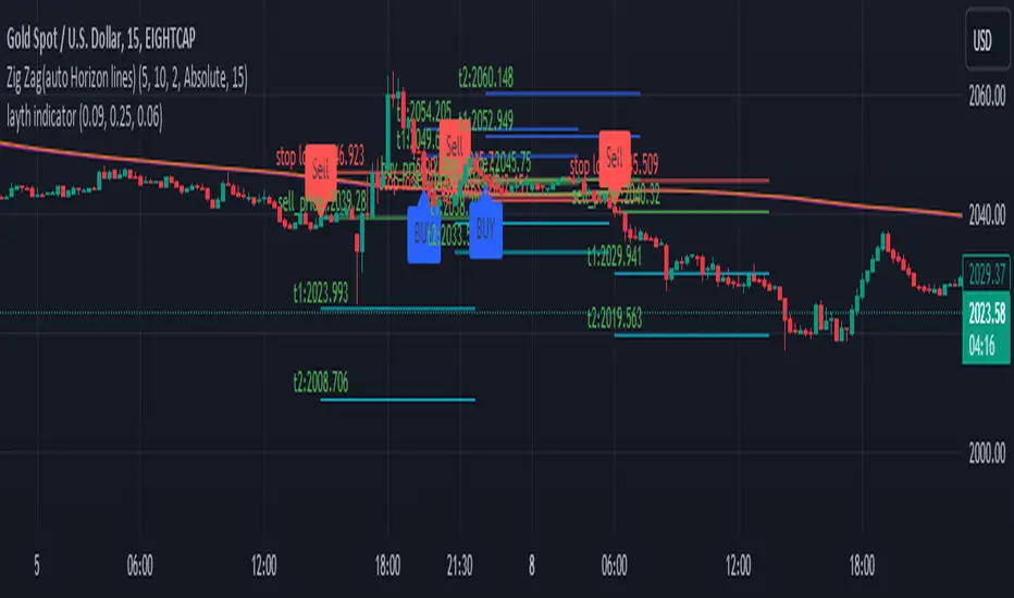
The indicator provides a buy signal when the price stabilizes above the moving averages. It should be close to the averages at the same time to ensure a close stop loss.
When the conditions are met, a long trade is opened, and the buy signal appears on the indicator. The stop loss is placed with the red line, and the targets are indicated with the blue balloons. Usually, the first target is twice the stop loss, and the second target is three times the stop loss.
This indicator is one of the most powerful indicators for monitoring price explosions in gold.
For clarification, this indicator is used (according to its default settings) exclusively for gold and only on the 15-minute timeframe. The indicator is created by Mr. Layth Al-Muhandis:
The indicator provides a very close stop loss compared to the first and second targets. I recommend adhering strictly to the stop loss and securing the trade after achieving profits.
This is a simple explanation of how the indicator works.
طريقة عمل المؤشر:
يوفر المؤشر إشارة شراء عند استقرار السعر فوق المتوسطات المتحركة. يجب أن يكون السعر قريبًا من المتوسطات في نفس الوقت لضمان وجود استوب لوس قريب.
عند تحقيق الشروط، يتم فتح صفقة شراء، وتظهر إشارة الشراء على المؤشر. يتم وضع الاستوب لوس بالخط الأحمر، وتوضح البالونات الزرقاء الأهداف. عادةً، يكون الهدف الأول ضعف الاستوب لوس، والهدف الثاني ثلاثة أضعاف الاستوب.
هذا المؤشر من بين أقوى المؤشرات لرصد انفجارات الأسعار في الذهب.
للتنويه، يُستخدم هذا المؤشر (وفقًا لإعداداته الافتراضية) حصريًا للذهب وعلى فاصل زمني 15 دقيقة فقط. تم إنشاء المؤشر بواسطة السيد ليث المهندس.
يوفر المؤشر استوب لوس قريب جداً مقارنة بالهدف الأول والهدف الثاني. أنصح بالالتزام الصارم بالاستوب لوس وتأمين الصفقة بعد تحقيق الأرباح.
Cari dalam skrip untuk "GOLD"
XAUXXXThis simple script is meant to get around the limitations some data providers have, in terms of the length of historical data they choose to provide traders. Inspired by OANDA's XAUCAD pair only having data as far back as 2005, whereas XAUUSD has data back to to the 19th century.
By taking the OHLC data from XAUUSD and multiplying it by the price of USD in a desired currency you are able to see further back in time, the limitation now being the length of FX data available instead of the price of Precious metal / currency pair. As shown in the chart you can now see the price of Gold in CAD as far back as the late 1960s, a nearly half century of data uncovered for all to see!

The Golden Candlestick PatternThe Golden pattern is a three-candlestick configuration based on a variation of the golden ratio (2.618) from the Fibonacci sequence.
The bullish Golden pattern is composed of a normal bullish candlestick with any type of body, followed by a bigger bullish candlestick with a close price that is at least 2.618 times the size of the first candlestick (high to low). Finally, there must be an important condition that is, a third candlestick that comes back to test the open of the second candlestick from where the entry is given.
The bearish Golden pattern is composed of a normal bearish candlestick with any type of body, followed by a bigger bearish candlestick with a close price that is at least 2.618 times the size of the first candlestick (high to low). Finally, there must be an important condition that is, a third candlestick that comes back to test the open of the second candlestick from where the entry is given.

Multi-Symbol Cross Indicator Template - Unleash Your Potential!Unlock your full trading potential with this powerful and versatile Multi-Symbol Cross Indicator Template! This script is designed to make you stand out from the crowd by enabling you to monitor multiple symbols on a single chart for specific events, such as a Golden Cross or Death Cross. With its high adaptability to include various technical indicators, you're in complete control of your trading decisions and market analysis.
By using the built-in request.security function, this template fetches data for your chosen symbols from the selected exchange and calculates the conditions (e.g., moving average crossovers) for each symbol. Although the current implementation focuses on Golden Crosses and Death Crosses, the sky is the limit when it comes to modifying the script to incorporate other technical indicators such as RSI, MACD, or Bollinger Bands.
You, as a discerning trader, can easily customize the script by selecting your preferred exchange and symbols through input options. This flexibility allows you to monitor your favorite markets without the need for any direct code modification, giving you the ultimate adaptability for various trading strategies and market analysis purposes.
Remember, this script is more than just an example or template; it's the key to unleashing your inner trading genius. While it's not intended to be a standalone trading strategy, it serves as the foundation for you to build upon and create your own customized multi-symbol indicators or strategies. You are awesome, and with this Multi-Symbol Cross Indicator Template, there's no doubt that you're on the path to achieving great success in your trading journey!

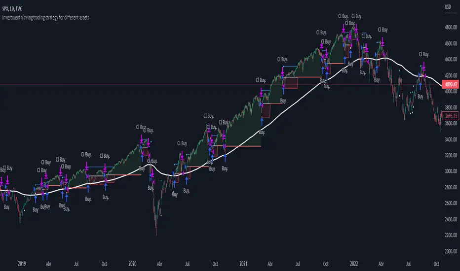
Investments/swing trading strategy for different assetsStop worrying about catching the lowest price, it's almost impossible!: with this trend-following strategy and protection from bearish phases, you will know how to enter the market properly to obtain benefits in the long term.
Backtesting context: 1899-11-01 to 2023-02-16 of SPX by Tvc. Commissions: 0.05% for each entry, 0.05% for each exit. Risk per trade: 2.5% of the total account
For this strategy, 5 indicators are used:
One Ema of 200 periods
Atr Stop loss indicator from Gatherio
Squeeze momentum indicator from LazyBear
Moving average convergence/divergence or Macd
Relative strength index or Rsi
Trade conditions:
There are three type of entries, one of them depends if we want to trade against a bearish trend or not.
---If we keep Against trend option deactivated, the rules for two type of entries are:---
First type of entry:
With the next rules, we will be able to entry in a pull back situation:
Squeeze momentum is under 0 line (red)
Close is above 200 Ema and close is higher than the past close
Histogram from macd is under 0 line and is higher than the past one
Once these rules are met, we enter into a buy position. Stop loss will be determined by atr stop loss (white point) and break even(blue point) by a risk/reward ratio of 1:1.
For closing this position: Squeeze momentum crosses over 0 and, until squeeze momentum crosses under 0, we close the position. Otherwise, we would have closed the position due to break even or stop loss.
Second type of entry:
With the next rules, we will not lose a possible bullish movement:
Close is above 200 Ema
Squeeze momentum crosses under 0 line
Once these rules are met, we enter into a buy position. Stop loss will be determined by atr stop loss (white point) and break even(blue point) by a risk/reward ratio of 1:1.
Like in the past type of entry, for closing this position: Squeeze momentum crosses over 0 and, until squeeze momentum crosses under 0, we close the position. Otherwise, we would have closed the position due to break even or stop loss.
---If we keep Against trend option activated, the rules are the same as the ones above, but with one more type of entry. This is more useful in weekly timeframes, but could also be used in daily time frame:---
Third type of entry:
Close is under 200 Ema
Squeeze momentum crosses under 0 line
Once these rules are met, we enter into a buy position. Stop loss will be determined by atr stop loss (white point) and break even(blue point) by a risk/reward ratio of 1:1.
Like in the past type of entries, for closing this position: Squeeze momentum crosses over 0 and, until squeeze momentum crosses under 0, we close the position. Otherwise, we would have closed the position due to break even or stop loss.
Risk management
For calculating the amount of the position you will use just a small percent of your initial capital for the strategy and you will use the atr stop loss for this.
Example: You have 1000 usd and you just want to risk 2,5% of your account, there is a buy signal at price of 4,000 usd. The stop loss price from atr stop loss is 3,900. You calculate the distance in percent between 4,000 and 3,900. In this case, that distance would be of 2.50%. Then, you calculate your position by this way: (initial or current capital * risk per trade of your account) / (stop loss distance).
Using these values on the formula: (1000*2,5%)/(2,5%) = 1000usd. It means, you have to use 1000 usd for risking 2.5% of your account.
We will use this risk management for applying compound interest.
In settings, with position amount calculator, you can enter the amount in usd of your account and the amount in percentage for risking per trade of the account. You will see this value in green color in the upper left corner that shows the amount in usd to use for risking the specific percentage of your account.
Script functions
Inside of settings, you will find some utilities for display atr stop loss, break evens, positions, signals, indicators, etc.
You will find the settings for risk management at the end of the script if you want to change something. But rebember, do not change values from indicators, the idea is to not over optimize the strategy.
If you want to change the initial capital for backtest the strategy, go to properties, and also enter the commisions of your exchange and slippage for more realistic results.
If you activate break even using rsi, when rsi crosses under overbought zone break even will be activated. This can work in some assets.
---Important: In risk managment you can find an option called "Use leverage ?", activate this if you want to backtest using leverage, which means that in case of not having enough money for risking the % determined by you of your account using your initial capital, you will use leverage for using the enough amount for risking that % of your acount in a buy position. Otherwise, the amount will be limited by your initial/current capital---
Some things to consider
USE UNDER YOUR OWN RISK. PAST RESULTS DO NOT REPRESENT THE FUTURE.
DEPENDING OF % ACCOUNT RISK PER TRADE, YOU COULD REQUIRE LEVERAGE FOR OPEN SOME POSITIONS, SO PLEASE, BE CAREFULL AND USE CORRECTLY THE RISK MANAGEMENT
Do not forget to change commissions and other parameters related with back testing results!
Some assets and timeframes where the strategy has also worked:
BTCUSD : 4H, 1D, W
SPX (US500) : 4H, 1D, W
GOLD : 1D, W
SILVER : 1D, W
ETHUSD : 4H, 1D
DXY : 1D
AAPL : 4H, 1D, W
AMZN : 4H, 1D, W
META : 4H, 1D, W
(and others stocks)
BANKNIFTY : 4H, 1D, W
DAX : 1D, W
RUT : 1D, W
HSI : 1D, W
NI225 : 1D, W
USDCOP : 1D, W
Recession Warning Traffic LightThis is an indicator that uses 6 different metrics to determine the combined probability of a recession and compares the high probability warning periods against actual historical periods of recession.
GREEN tells us that the referenced recession indicators are not exhibiting any warning. Observe the long stretches of “all-green” in between recessionary periods in the chart above.
RED will show a full-on warning level for that particular recession indicator, signaling that monitoring of this sector is clearly showing a problem – which has in the past, reliably exhibited itself as a forewarning of recessions.
Adding green and red together can help determine a combined probability of recession.
IMPORTANT: Your chart should be on 1d and set to SPX , DJI ,or NDQ indices
Precious metals: This indicator calculates the relative prices of Gold & rhodium. Gold is a flight-to-quality asset. Rhodium is the rarest of precious industrial metals and prices spike when the economy is heating up. In front of a recession, the upper relative movement of rhodium precedes gold.
Stock markets: This indicator compares closing prices to growth rate curves of the SPX. This indication is the noisiest but tells us very well when the recession has ended. Stock market indices, which respond to “smart money” moving out of markets when the other indicators begin to warn of recession, or when markets become overheated and rise to historically unsustainable levels.
Yield curve: This indicator compares the 3m & 10y treasuries and detects yield curve inversions. Interest rates are controlled by the Federal Reserve and by the purchasers in the Federal Treasury auction markets, which together create the treasury yield curve. This inversion is the most reliable recession indicator. These happen during a flight to quality.
Federal Reserve: This indicator measures GDP and detects contraction which is technically a recession. This is usually one of the last indicators to enter a Warning state, and it could be 6 months delayed simply confirming what may have already been projected.
Money Supply. This indicator measures the M2 money supply, which typically grows about 1% per calendar quarter. When this shrinks, it's tapping the brakes on the economy. This can also lead to yield curve inversion. This is also a measure of inflation and its effects on the aggregate money supply (liquid capital) available for short-term economic activity, or which can be directed into the purchase of long-term, less liquid assets.
Leading Economic factors: There is a whole basket of leading economic indicators that, as collections, reflect overall growth or contraction of economic activity. These indicators include measures of level and growth in productivity, employment, housing, consumer confidence, industrial purchasing confidence, and much more. These indicators may or may not be detached from the broader economy, and often provide up to 6 months of foresight. For more information please visit www.conference-board.org
Actual Recession: Central Bank indicators are published by the Federal Reserve and reflect their own analysis of national and regional economic health, as well as their calculations of the likelihood of a recession. The Federal Reserve has a recession ticker which is used to plot periods of actual recessions on this indicator for comparison.

In Chart Currency TickersQuick View of Multiple Currencies & Gold Price on Chart
In Chart Currency Tickers will help quick view of Multiple Currencies (Up/Down points & Percentage), you can change symbols on settings as per your requirement
മെയിൻ കറൻസികളും സ്വർണവിലയും റിയൽ ടൈം മോണിറ്റർ ചെയ്യുന്നതിനും മാർക്കറ്റ് സെന്റിമെൻറ് അറിയുന്നതിനും അതിനനുസരിച്ച് ട്രേഡിങ്ങ് ഡിസിഷൻ എടുക്കുന്നതിനും നിങ്ങളെ സഹായിക്കുന്നു
Happy Trading to All..!!!
Asif Kerim Naduvilaparambil

EMA ON MA SETSOORY FOR MY EINGLISH
ITS NOT MY NATIVE AND IM NOT GOING TO GOOGLE TRANSLATE THIS
this is a beuaitful indicator that plot EMA that gat is calc from another ma and length for your choise so you will get an = 'ema on ma '
it can plot you more beautiful results and more smoothing results
i added golden/death cross for all ma
enjoy !
היי חברים זה בעצם אינדיקטור של ממוצע נע על ממוצע נע לנוחיכותכם
הפלט הראשי הוא EMA
הוא לוקח את החישוב שלו ממוצע אחר והאורך שתגדירו
נותן תוצאה יותר חלקה של ממוצעים נעים
הוספתי חתיוכים בין ההמוצעים
תהנו.
Find Best Performing MA For Golden CrossHello!
This script calculates the performance of any asset following a golden cross of two moving averages of any length!
The calculated moving averages are: SMA, EMA, HMA, VWMA, WMA, LSMA, and ALMA
The best performing moving average for the selected data series is listed first, followed by a descending order.
The indicator works on any timeframe, any asset, and can even be used on indicators such as RSI, %b, %k, etc.
The Moving Average Length and Source Are Customizable!
The Moving Averages Can Be Plotted on Most Data Series, Such As:
Close, Open, Low, hlc3, RSI, %B, %K, Etc.
The Script Will Recalculate for the Timeframe (1m, 5m, D, etc.)!
The (XX Candles) Indicates the Average Number of
Sessions the Shorter Ma Remains Above the Longer Ma Following an Upside Cross!
The Percentages (XX.XX%) Indicate the Average
Percentage Price Gain/Loss Following a Golden Cross,
Until the Shorter Ma Crosses Back Under the Longer Ma!
In This Example I Am Using a 63 Session Length for the
Shorter Ma for All Listed Ma Types for Closing Prices, and a 196 Candle Length for the Longer Ma!

Bitcoin Golden Bottom Oscillator (MZ BTC Oscillator)This indicator uses Elliot Wave Oscillator Methodology applied on "BTC Golden Bottom with Adaptive Moving Average" and Relative Strength Index of Resulted EVO to form an Oscillator to detect trend health in Bitcoin price. Ticker is set to "INDEX : BTCUSD" on 1D timeframe.
Methodology
Oscillator uses Adaptive Moving Average with 1 year of length, Minor length of 50 and Major length of 100 to mark AMA as Golden Bottom.
Percentage Elliot Wave Oscillator is calculated between BTC price and AMA.
Relative Strength Index of EVO is calculated to detect trend strength and divergence detection.
Hull Moving Average of resulted RSI is used to smoothen the Oscillator.
Oscillator is hard coded to 'INDEX:BTCUSD' ticker on 1d so it can be used on any other chart and on any other timeframe.
Color Schemes
Bright Red background color indicates that price has left top Fib multiple ATR band and possibly go for top.
Light Red background color indicates that price has left 2nd top Fib multiple ATR band and possibly go for local top.
Lime background color indicates that price has entered lowest band indicating local bottom.
Bright Green background color indicates that price is approximately resting on Golden Bottom i.e. AMA.
Oscillator color is set to gradient for easy directional adaption.
BTC Golden Bottom with Adaptive Moving Average

Baekdoo golden diamond signalHi forks,
I'm trader Baekdoosan who trading Equity from South Korea. This Baekdoo golden Diamond signal indicate good buying position to trade.
Here's the ideas
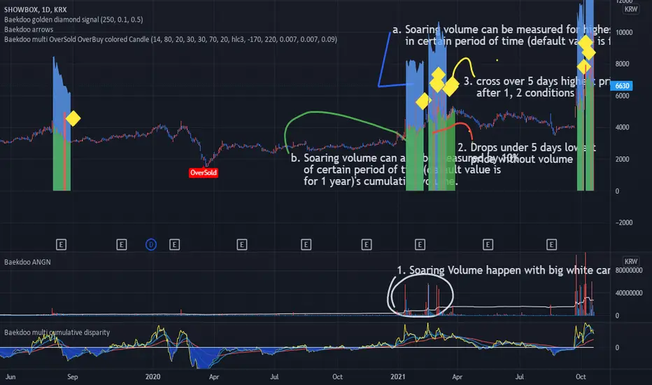
1. Soaring volume happen with big white candle.
a. Soaring volume can be measured for highest volume in certain period of time (default value is for 1 year). (blue area)
b. Soaring volume can also be measured by 10% of certain period of time(default value is for 1 year)'s cumulative volume . (green area) => you can adjust this ratio input. the higher value is the more likely to trail of whale
2. Drops under 5 days lowest price without volume . (red area) => I put half of average volume as default but you may can adjust it (the lower value is the more likely to soar again)
3. cross over 5 days highest price after 1, 2 conditions => Golden Diamond
underneath of this idea is, big chunk of the money comes and correction is on going but major whale's amount hold tight.
you can modify input values based on your investigation. It works well on day chart as well as minute chart. for the area with breaks plots are to checking the 1,2 conditions. so for final indicator will only be shown from this indicator but you can select plots if you think that is useful.
hope this will help your trading on equity as well as crypto. I didn't try it on futures . Best of luck all of you. Gazua~!
Baekdoo Golden Diamond signalHi forks,
I'm trader Baekdoosan who trading Equity from South Korea. This Baekdoo golden Diamond signal indicate good buying position to trade.
Here's the ideas
1. Soaring volume happen with big white candle.
a. Soaring volume can be measured for highest volume in certain period of time (default value is for 1 year). (blue area)
b. Soaring volume can also be measured by 10% of certain period of time(default value is for 1 year)'s cumulative volume. (green area) => you can adjust this ratio input. the higher value is the more likely to trail of whale
2. Drops under 5 days lowest price without volume. (red area) => I put half of average volume as default but you may can adjust it (the lower value is the more likely to soar again)
3. cross over 5 days highest price after 1, 2 conditions => Golden Diamond
underneath of this idea is, big chunk of the money comes and correction is on going but major whale's amount hold tight.
you can modify input values based on your investigation. It works well on day chart as well as minute chart. for the area with breaks plots are to checking the 1,2 conditions. so for final indicator will only be shown from this indicator but you can select plots if you think that is useful.
hope this will help your trading on equity as well as crypto. I didn't try it on futures . Best of luck all of you. Gazua~!

Auto Fib Golden Pocket Band - Strategy with Buy Signalsthis strategy is based on the Indicator "Auto Fib Golden Pocket Band - "Autofib Moving Average"
it's the same as the indicator but with:
- the strategy tester included
- several entry Signal filter
- Dynamic SL

Center Of Gravity OscillatorThe COG Oscillator (center of gravity) is an indicator based on statistics and the Fibonacci golden ratio. It uses ALMA as a trigger and LSMA as "zero line". The trigger is set tight by default but can be tweaked by adjusting the window size and sigma in settings. This is a great indicator for setting up trades and spotting reversals. There are 2 main strategies that come with this indicator:
Strategy 1: Long positions are entered when current low point is higher than previous low. Short positions are entered as current high is lower than previous high. (Shown in image above)
Strategy 2 : If market is bullish long trades are entered as COG line crosses over red LSMA line. Traders have the option of scalping the first crossover or even scaling out of trade to close on second exit. This works the opposite for shorts when market is bearish.
Above shows different configurations of the indicator. Top shows length of 50, Middle has length of 21 and bottom is default 9.

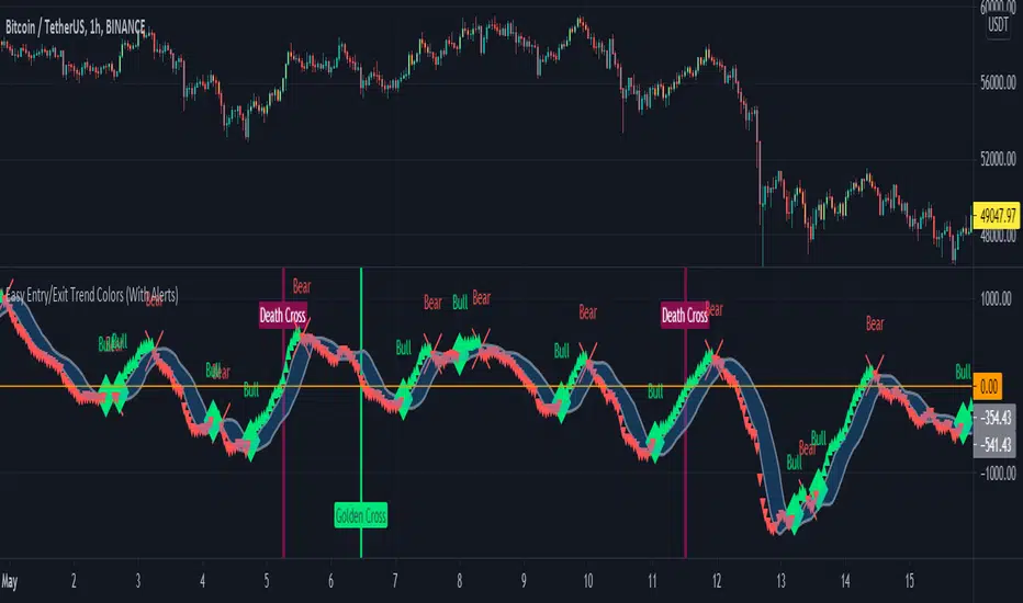
Easy Entry/Exit Trend Colors (With Alerts)This is an updated version of user Algokid's script called 'AK MACD BB INDICATOR V 1.00'. You can find that original script here:
I added many alerts along with the Bullish and Bearish alerts when the MACD crosses over the Upperband or crosses down on the Lowerband.
I personally use this indicator with Crypto charts (Bitcoin on a 15min, 1hour, and 4 hour timeframe) as one of many confirmations that it's a good time to enter a trade. This script was made to be easy to follow with the colors of GREEN triangles being a good uptrend or entry confirmation, and RED being a confirmation to sell/short or exit your trade.
It's important to use this indicator in combination with other indicators that can give you more confirmations to enter or exit a trade, and make sure you are on normal candles and not HA or any other candles as you can get wildly inaccurate results.
This script also has the Death & Golden crosses, which is the slow and fast moving averages crossing over each other. I don't use this as an additional confirmation, it's just nice to know where the cross happens.
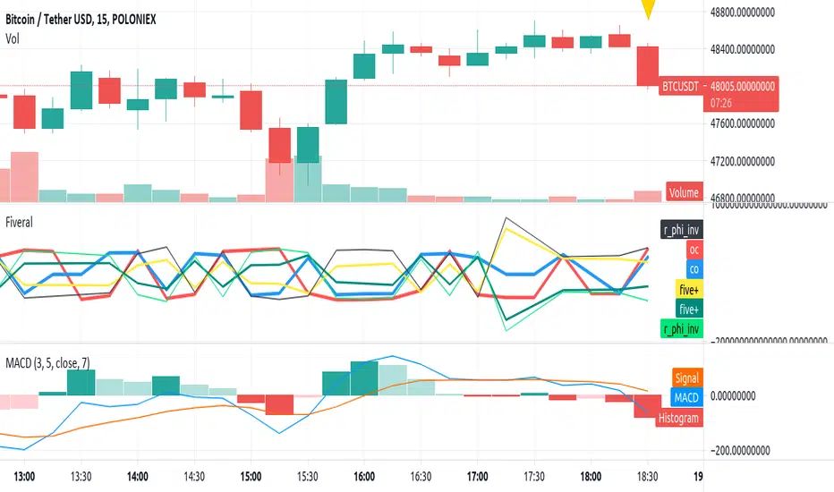
Fiveral: Repulsion/Golden Radio HackAnother in a series of experimental indicators using logarithmic scale visualisation.
This one extends into some work on I've been doing on 'the cube', but Pine isn't liking multiple log lines even when the equations are included for each plotted variable, meaning, no variables used in the definition of a variable, as is done here. As a result, accuracy of this indicator can't be guaranteed between scales, or during use.
Have at it, and enjoy!
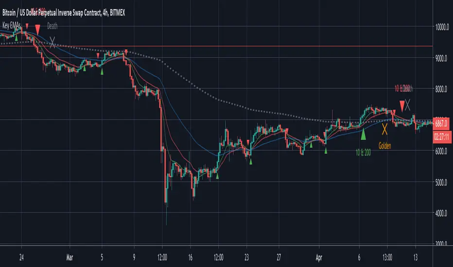
Key EMAsSimple trade helper script that plots:
- 10 & 20 EMA crosses for fast moves
- 10 & 200 EMA crosses for trends
- 50 & 200 EMA golden and death crosses
Alerts built in.
Moving Averages CrossThis Indicator helps you spot crosses between moving averages.
Thought to combine short term and long term strategies.
A complementary element for your trading tool belt.
The First study (short term):
Helps you visualise the relation between two simple moving averages (9,21) by default.
The Second study (long term):
Helps you identify the relation between three simple moving averages (50,100, 200) by default.
Spot Golden Crosses and Death Crosses from far.

Bollinger Band Strategy (Basic) Version 1 This strategy is for learning purposes only. Pay special attention to these strategies on longer aggregation periods (like 1 hr chart or more). Don't expect accurate results when you set a limit to 10 cents above your entry to be accurate. For example if you set the chart to 1 day, the price may move down and hit a stop 10 times then tag your limit. If this doesn't make sense, just don't use strategies here. Learn more first. That being said, I don't have specific recommendations for each aggregation period, backtesting isn't always perfect.
Now then, this strategy can be used as the traditional BB method by setting the "Stop" and "Limit Out" to like 10000, check "Reversal Entry" and uncheck "Limit Time of Day" This will keep the strategy running just reverse your position when price crosses outside each band.
INPUTS:
Length - length of WMA that I used for mean of Bollinger Band (this may suppose to be SMA, too bad)
Source - O-H-L-C basis for WMA
Deviation - normal Standard deviation that would be set when using Bollinger Band
Trailing stop check box - your stop value will be either a hard stop or trailing stop for an exit
Stop - the stop value - remember you can set this really high and it won't stop out
Limit Out - the limit value for exit
Reversal Entry check box - This changes each entry from a reversal (traditional idea of BB) to enter a trend trade - hopefully version 2 will have choice to trend one direction and reversal in the other.
Limit Time of Day - Especially when trading futures, you may want to only trade a specific time of day, when this box is checked, you can set the entry times below, exit will still only occur based on limit/stop or a flip entry order (the opposite entry condition is met)
Tips:
when I don't know a thing about a price range, like gold. I can set the limit out to 10000 and play with a trailing stop to get a better idea of what is even possible before tuning further.


Kringold2[WOZDUX] gold equivalentThe indicator is a tool for global analysis. The default is the price of gold. The price of the instrument from the main window is divided by the price of gold. The result is the price of the instrument in units of gold. The screen uses the Dow Jones index as an example. In the indicator window, the price of the index in units of gold or the so-called gold Dow Jones. The use of the gold equivalent makes it possible to see more truthful trends. The Indicator has the ability to change gold to any other equivalent. It is enough to change the name of the exchange and the name of the instrument in the options tool and exchange. In addition, in the settings, the second box on top allows you to view the graph in a linear or logarithmic scale. The first box at the top switches the line chart or the CCI =WT indicator to this chart.
-------------------------------------------
Индикатор это инструмент для глобального анализа. По умолчанию используется цена золота. Цена инструмента из основного окна делится на цену золота. В результате получается цена инструмента в единицах золота. На экране для примера используется индекс Доу джонса. В окне индикатора цена индекса в единицах золота или так называемый золотой Доу Джонс. Использование золотого эквивалента дает возможность видеть более правдивые тенденции движения. В Индикаторе есть возможность поменять золото на любой другой эквивалент. Достаточно в опциях инструмент и биржа изменить название биржи и название инструмента. Кроме того, в настройках, второй бокс сверху дает возможность смотреть график в линейном или логарифмическом масштабе. Первый бокс сверу переключает линейный график или индикатор CCI =WT к данному графику.
