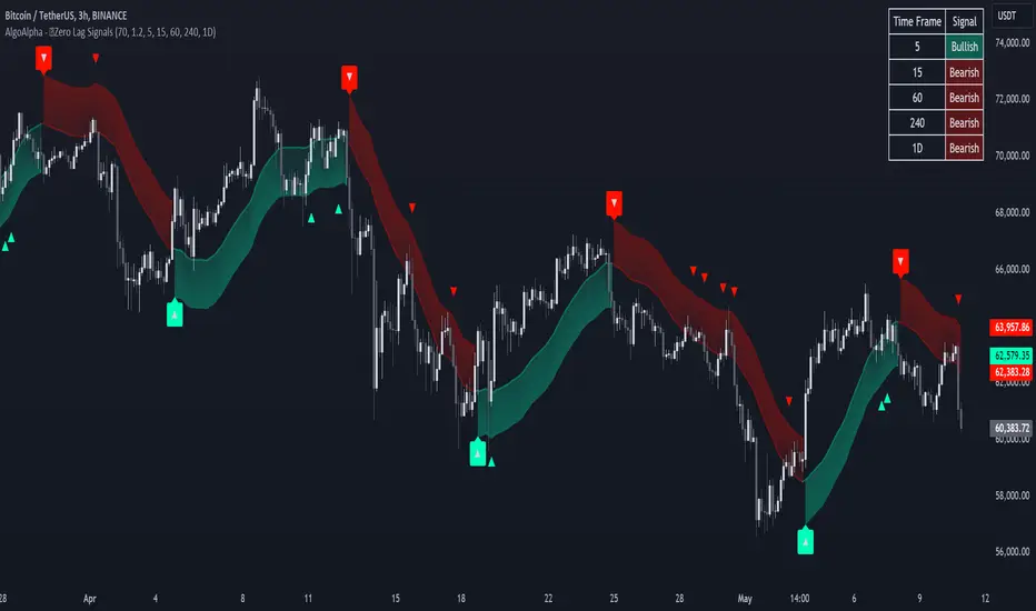
Zero Lag Trend Signals (MTF) [AlgoAlpha]Zero Lag Trend Signals 🚀📈
Ready to take your trend-following strategy to the next level? Say hello to Zero Lag Trend Signals , a precision-engineered Pine Script™ indicator designed to eliminate lag and provide rapid trend insights across multiple timeframes. 💡 This tool blends zero-lag EMA (ZLEMA) logic with volatility bands, trend-shift markers, and dynamic alerts. The result? Timely signals with minimal noise for clearer decision-making, whether you're trading intraday or on longer horizons. 🔄
🟢 Zero-Lag Trend Detection : Uses a zero-lag EMA (ZLEMA) to smooth price data while minimizing delay.
⚡ Multi-Timeframe Signals : Displays trends across up to 5 timeframes (from 5 minutes to daily) on a sleek table.
📊 Volatility-Based Bands : Adaptive upper and lower bands, helping you identify trend reversals with reduced false signals.
🔔 Custom Alerts : Get notified of key trend changes instantly with built-in alert conditions.
🎨 Color-Coded Visualization : Bullish and bearish signals pop with clear color coding, ensuring easy chart reading.
⚙️ Fully Configurable : Modify EMA length, band multiplier, colors, and timeframe settings to suit your strategy.
How to Use 📚
⭐ Add the Indicator : Add the indicator to favorites by pressing the star icon. Set your preferred EMA length and band multiplier. Choose your desired timeframes for multi-frame trend monitoring.
💻 Watch the Table & Chart : The top-right table dynamically updates with bullish or bearish signals across multiple timeframes. Colored arrows on the chart indicate potential entry points when the price crosses the ZLEMA with confirmation from volatility bands.
🔔 Enable Alerts : Configure alerts for real-time notifications when trends shift—no need to monitor charts constantly.
How It Works 🧠
The script calculates the zero-lag EMA (ZLEMA) by compensating for data lag, giving traders more responsive moving averages. It checks for volatility shifts using the Average True Range (ATR), multiplied to create upper and lower deviation bands. If the price crosses above or below these bands, it marks the start of new trends. Additionally, the indicator aggregates trend data from up to five configurable timeframes and displays them in a neat summary table. This helps you confirm trends across different intervals—ideal for multi-timeframe analysis. The visual signals include upward and downward arrows on the chart, denoting potential entries or exits when trends align across timeframes. Traders can use these cues to make well-timed trades and avoid lag-related pitfalls.
Cari dalam skrip untuk "Table"
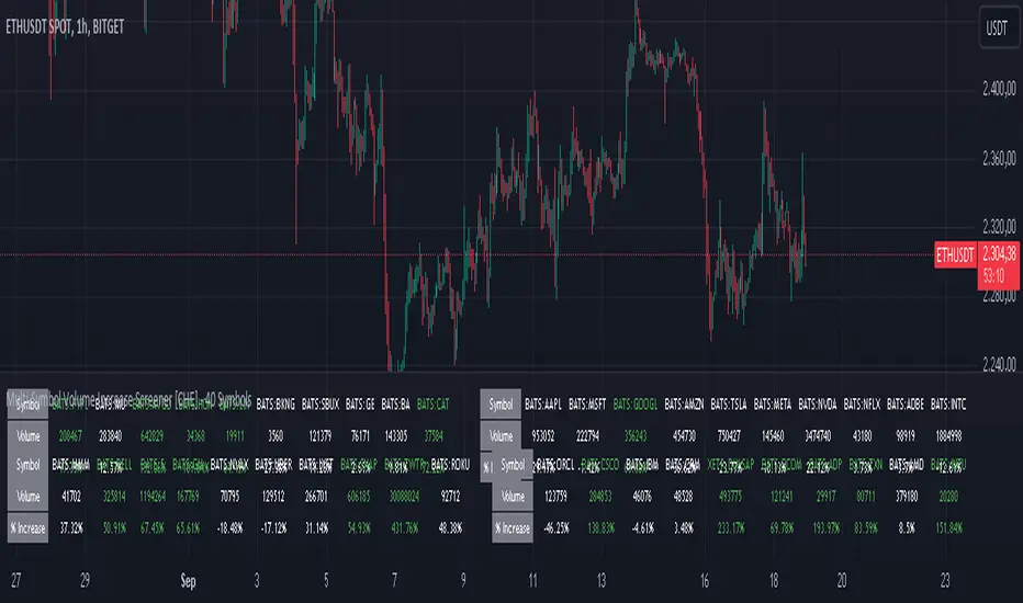
Multi-Symbol Volume Increase Screener [CHE] MultiSymbol Volume Increase Screener
Designed for TradingView
Presented by Chervolino
Introduction
Welcome to the presentation of the MultiSymbol Volume Increase Screener—a powerful tool designed to enhance your trading strategy on TradingView. Developed at the request of jscott143, this screener provides traders with realtime insights into significant volume movements across multiple symbols, enabling more informed and timely trading decisions.
Purpose and Objectives
Identify HighVolume Opportunities: Detect symbols experiencing a significant increase in volume compared to their historical average.
Monitor Multiple Symbols Simultaneously: Efficiently track up to five symbols in one view.
RealTime Alerts: Receive instant notifications when predefined volume conditions are met.
Comprehensive Overview: Display volume data and percentage increases in an organized table for easy analysis.
Key Features
1. MultiSymbol Monitoring
Track up to five different symbols simultaneously.
Customize the list of symbols based on your trading portfolio.
2. Volume Analysis
Compare current candle volume against the average volume over a specified period.
Calculate and display the percentage increase in volume.
3. RealTime Alerts
Set a volume increase multiplier (e.g., 1.5x) to trigger alerts.
Receive alerts via email, popup, or SMS when conditions are met.
4. UserFriendly Table Display
View symbols, their current volume, and percentage increase in a clear, concise table.
Colorcoded indicators highlight significant volume changes.
5. Customizable Parameters
Adjust the average volume period to suit different trading strategies.
Set your preferred volume increase multiplier for alerts.
How It Works
1. User Inputs:
Symbols Selection: Choose up to five symbols you wish to monitor.
Average Volume Period: Define the number of bars over which the average volume is calculated (default is 20).
Volume Increase Multiplier: Set the threshold for volume increase to trigger alerts (default is 1.5x).
2. Volume Calculation:
The screener fetches the current volume and calculates the simple moving average (SMA) of volume over the defined period for each symbol.
It then determines if the current volume exceeds the average volume by the specified multiplier.
3. Data Display:
A table is generated on the chart displaying each symbol, its current volume, and the percentage increase.
Green text indicates that the volume increase condition has been met.
4. Alert Generation:
When a symbol's current volume surpasses the average volume by the set multiplier, an alert is triggered.
Alerts are customizable and can be set to notify you through various channels.
Benefits
Enhanced DecisionMaking: Quickly identify highvolume trading opportunities across multiple assets.
Time Efficiency: Monitor several symbols without the need to switch between charts.
Proactive Trading: Stay informed with realtime alerts, allowing for timely trading actions.
Customization: Tailor the screener settings to align with your unique trading strategies and preferences.
Setup Instructions
1. Add the Screener to TradingView:
Navigate to TradingView and open the Pine Editor.
Add the MultiSymbol Volume Increase Screener indicator to your chart.
Save and apply the indicator.
2. Configure User Inputs:
Select up to five symbols you wish to monitor in the input fields "Symbol 1" to "Symbol 5".
Adjust the "Average Volume Period" and "Volume Increase Multiplier" as needed.
3. Set Up Alerts:
Click on the Alarm icon (🔔) in the TradingView toolbar.
In the "Condition" dropdown, select the "MultiSymbol Volume Increase Screener".
Choose the specific alert condition for each symbol (e.g., "Volume Increase Alert for Symbol 1").
Configure the alert actions (e.g., email, popup, SMS) and click "Create".
Repeat this process for each symbol you wish to monitor.
Visual Demonstration
Table Display Example:
| Symbol | Volume | % Increase |
| AAPL | 150,000 | 50.00% |
| MSFT | 120,000 | 20.00% |
| GOOGL | 180,000 | 80.00% |
| AMZN | 130,000 | 30.00% |
| TSLA | 160,000 | 60.00% |
Green Text: Indicates that the volume increase condition has been met for that symbol.
Alert Notification Example:
```
🚀 Symbol 1 shows a volume increase!
```
Note: Replace "Symbol 1" with the actual symbol as per your configuration.
Customization Options
Increase the Number of Symbols:
While the current screener monitors five symbols, it can be extended to monitor more by adding additional input fields and corresponding calculations. However, be mindful of TradingView's Pine Script limitations and potential performance impacts.
Adjust Volume Period and Multiplier:
Tailor the "Average Volume Period" and "Volume Increase Multiplier" to align with your specific trading strategies and market conditions.
Enhance Table Information:
Incorporate additional data points such as current price, price change percentage, or other technical indicators to enrich your analysis.
Benefits of Using the Screener
Efficiency: Saves time by providing a consolidated view of multiple symbols' volume activity.
Proactive Trading: Enables you to act swiftly on significant volume movements, which often precede price changes.
DataDriven Decisions: Facilitates informed trading decisions based on realtime volume analysis.
Customization: Offers flexibility to adapt the screener to various trading styles and preferences.
Conclusion
The MultiSymbol Volume Increase Screener is an invaluable tool for traders looking to capitalize on significant volume movements across multiple assets. Developed at the request of jscott143, this screener integrates seamlessly with TradingView, providing realtime insights and alerts to enhance your trading strategy.
Q&A
Feel free to ask any questions or request further customization to better suit your trading needs.
Contact Information
Created for: jscott143
Thank you for your attention!
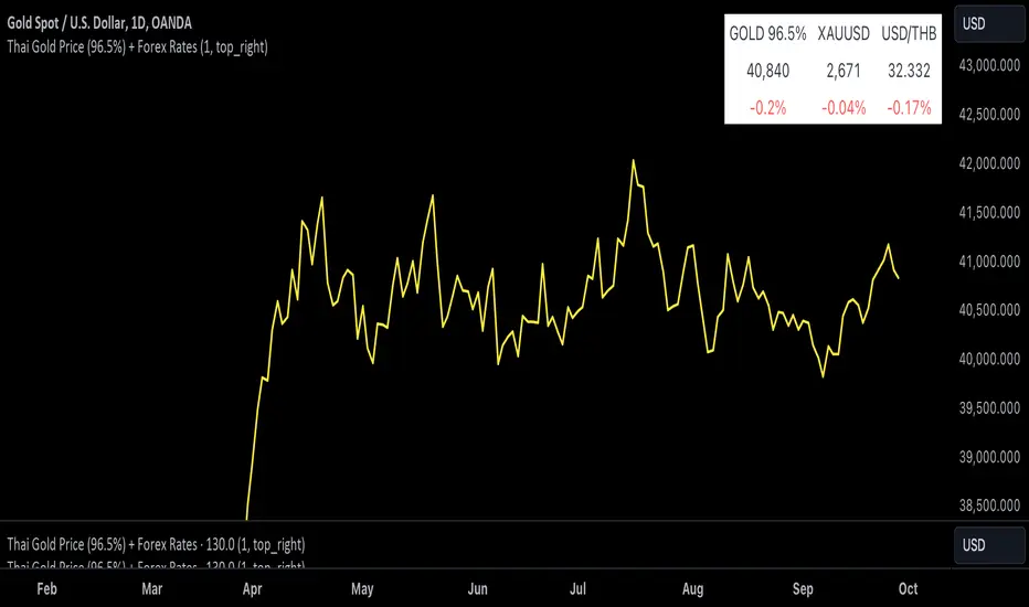
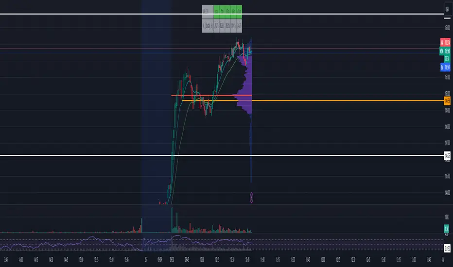
Thai Gold 96.5%Gold 96.5% Price Display (Test Version)
This Pine Script indicator is a test version designed to display the current price of Thai gold (96.5%) in a customizable table on your TradingView chart. The script calculates the gold price using the latest values for XAU/USD and USD/THB, reflecting the price of gold in Thai Baht (THB) with a purity adjustment.
Features:
- Price Calculation: Computes the Thai gold price by multiplying the XAU/USD price with USD/THB and adjusting for gold purity (0.49 * 0.965).
- Customizable Display: Adjust text size, text color, background color, and table position (Top Right, Top Left, Bottom Right, Bottom Left).
- Formatted Output: Gold price is formatted with commas for better readability.
Inputs:
- Text Size: Choose from tiny, small, normal, large, or huge.
- Text Color: Customize the text color.
- Background Color: Select a background color for the table.
- Table Position: Choose the table position on the chart.
Usage:
Add this test script to your TradingView chart to see the current Thai gold price displayed in a table format. This version is for testing purposes and may be updated based on feedback.
Feel free to test and customize the script further!
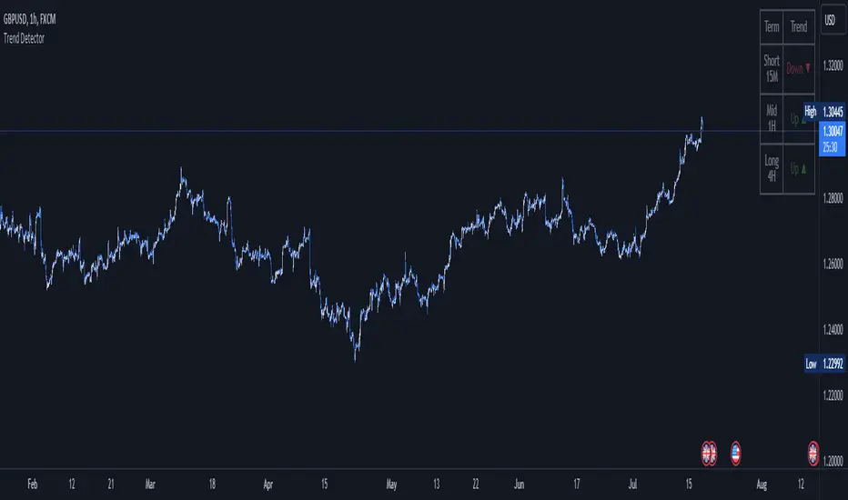
Trend DetectorThe Trend Detector indicator is a powerful tool to help traders identify and visualize market trends with ease. This indicator uses multiple moving averages (MAs) of different timeframes to provide a comprehensive view of market trends, making it suitable for traders of all experience levels.
█ USAGE
This indicator will automatically plot the chosen moving averages (MAs) on your chart, allowing you to visually assess the trend direction. Additionally, a table displaying the trend data for each selected MA timeframe is included to provide a quick overview.
█ FEATURES
1. Customizable Moving Averages: The indicator supports various types of moving averages, including Simple (SMA) , Exponential (EMA) , Smoothed (RMA) , Weighted (WMA) , and Volume-Weighted (VWMA) . You can select the type and length for each MA.
2. Multiple Timeframes: Plot moving averages for different timeframes on a single chart, including fast (short-term) , mid (medium-term) , and slow (long-term) MAs.
3. Trend Detector Table: A customizable table displays the trend direction (Up or Down) for each selected MA timeframe, providing a quick and easy way to assess the market's overall trend.
4. Customizable Appearance: Adjust the colors, frame, border, and text of the Trend Detector Table to match your chart's style and preferences.
5. Wait for Timeframe Close: Option to wait until the selected timeframe closes to plot the MA, which will remove the gaps.
█ CONCLUSION
The Trend Detector indicator is a versatile and user-friendly tool designed to enhance your trading strategy. By providing a clear visualization of market trends across multiple timeframes, this indicator helps you make informed trading decisions with confidence and trade with the market trend. Whether you're a day trader or a long-term investor, this indicator is an essential addition to your trading toolkit.
█ IMPORTANT
This indicator is a tool to aid in your analysis and should not be used as the sole basis for trading decisions. It is recommended to use this indicator in conjunction with other tools and perform comprehensive market analysis before making any trades.
Happy trading!
Time-itTime-it = Time based indicator
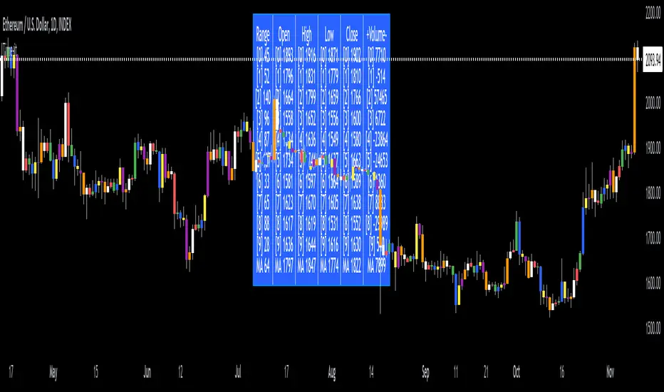
The Time-it indicator parses data by the day of week. Every tradeable instrument has its own personality. Some are more volatile on Mondays, and some are more bullish / bearish on Fridays or any day in between. The key metrics Time-it parses is range, open, high, low, close and +volume-.
The Time-it parsed data is printed in a table format. The table, position, size & color and text color & size can be changed to your preference. Each column parsed data is the last 10 which is numbered 0-9 which refers to the number of the selected day bars ago. For example: if Monday is chosen, 0 is the last closed Monday bar and 9 is the last closed Monday 9 Monday bars ago.
Range = measures the range between high and low for the day.
Open = is the opening price for the day.
High = is the high price for the day.
Low = is the low price for the day.
Close = is the closing price for the day.
+volume- = is the positive or negative volume for the day.
Default settings:
*Represents a how to use tooltip*
Source = ohlc4
* The source used for MA
MA length = 20
* The moving average used
Day bar color on / off
* checked on / unchecked off
Monday = blue
Tuesday = yellow
Wednesday = purple
Thursday = orange
Friday = white
Saturday = red
Sunday = green
Day M, T, W, TH, F, ST, SN.
* Parsed data for the day of week tables
Table, position, size & color:
Top, middle, bottom, left, center, right
* Table position on the chart.
Frame width & border width = 1
Text color and text size
Border color and frame color
Decimal place = 0
* example: use 0 for a round number, use 4 for Forex
*** The Time-it indicator uses parts and/or pieces of code from "Tradingview Up/Down Volume" and "Tradingview Financials on Chart".
Smart Money Breakouts [ChartPrime]The " Smart Money Breakouts " indicator is designed to identify breakouts based on changes in character (CHOCH) or breaks of structure (BOS) patterns, facilitating automated trading with user-defined Take Profit (TP) level.
the indicator incorporates essential elements such as volume analysis and a data table to assist traders in optimizing their strategies.
🔸 Breakout Detection:
The indicator scans price movements for "Change in Character" (CHOCH) and "Break of Structure" (BOS) patterns, signaling potential breakout opportunities in the market.
🔸User-Defined TP :
Traders can customize the Take Profit (TP) through the indicator settings, with these levels dynamically calculated based on the Average True Range (ATR). This allows for precise risk management and profit targets that adapt to market volatility.
🔸 Volume Analysis and Trade Direction Specific Analysis:
The indicator includes a volume checker that provides valuable insights into the strength of the breakout, taking into account trade direction.
🔸If the volume label is red and the trade is long, it suggests a higher likelihood of hitting the Stop Loss (SL).
🔸If the volume label is green and the trade is long, it indicates a higher probability of hitting the Take Profit (TP).
🔸For short trades, a red volume label suggests a higher likelihood of hitting TP, while a green label suggests a higher likelihood of hitting SL.
🔸A yellow volume label suggests that the volume is inconclusive, neither favoring bullish nor bearish movements.
🔸Data Table:
The indicator features a data table that keeps track of the number of winning and losing trades for specific timeframes or configurations.
This table serves as a valuable tool for traders to analyze performance and discover optimal settings and timeframes.
The "Smart Money Breakouts" indicator provides traders with a comprehensive solution for breakout trading, combining technical analysis of changes in character and breaks of structure, volume insights, and performance tracking while dynamically adjusting TP and SL levels based on market volatility through the ATR.

IU Probability CalculatorHow This Script Works:
1. This script calculate the probability of price reaching a user-defined price level within one candle with the help Normal Distribution Probability Table.
2. Normal Distribution Probability Table is use for calculating probability of events, it's very powerful for calculation of probability and this script is fully based on that table.
3. It takes the Average True Range value or Standard Deviation value of past user-defined length bar.
4. After that it take this formula z = ( price_level - close ) / (ATR or Standard Deviation) and return the value for z, for the bearish side it take z = (close - price level) / (ATR or Standard Deviation ) formula.
5. Once we have the z it look into Normal Distribution Probability Table and match the value.
6. Now the value of z is multiple buy 100 in order to make it look in percentage term.
7. After that this script subtract the final value with 100 because probability always comes under 100%
8. finally we plot the probability at the bottom of the chart the red line indicates "The probability of price not reaching that price level", While the green line indicates "Probability of price Reaching that level " .
9. This script will work fine for both of the directions
How This Is Useful For The User:
1. With this script user can know the probability of price reaching the certain level within one candle for both Directions .
2. This is useful while creating options hedging strategies
3. This can be helpful for deciding stop loss level.
4. It's useful for scalpers for managing their traders and it can be use by binary option traders.

Market Open - Relative VolumeThe indicator calculates the Pre-market volume percentage of the current day, relative to the average volume being traded in the trading session (14 days), displayed in Table Row 1, Table Cell 1, as V%. Pre-market volume between 15% & 30% has a orange background color. Pre-market volume percentage above 30% has a green background color.
The indicator calculates the relative volume per candle relative to the average volume being traded in that time period (14 days) (e.g., "1M," "2M," up to "5M"), displayed in a table. Relative volume between 250% & 350% has a orange background color. Relative volume above 350% has a green background color.
FYI >> Indicator calculations are per candle, not time unit (due to pine script restrictions). Meaning, the indicator current table data is only accurate in the 1M chart. If you are using the indicator in a higher timeframe, e.g., on the 5M chart, then the values in table cells >> (1M value == relative volume of the first 5-minute candle) (5M value = relative volume of the first five 5-minute candles) and so on. (Future versions will have a dynamic table).
Supertrend Targets [ChartPrime]The Supertrend Targets indicator combines the concepts of trend-following with dynamic volatility-based target levels. It takes core simple and classical concepts and provides actionable insights. The core of this indicator revolves around the "Supertrend" algorithm, which essentially uses the Average True Range (ATR) and a multiplier to determine if the price of a financial instrument is in an uptrend or downtrend. The indicator generates various plot points on the trading chart, which traders can use to make informed trading decisions.
Users can set several input parameters such as the source price, custom levels, multiplier scale, length of the average true range, and the window length. Traders can also opt to enable a table that shows numeric target data by percentiles, risk ratio, take profit and stop loss points.
The generated plots and fills on the chart represent various levels of potential gains and drawdowns, acting as potential targets for taking profit or stopping losses. These include the 25th, 50th, 75th, 90th, and 100th percentiles, which are adjustable by scale. There are also plots for average gain and drawdown levels, enhanced by standard deviation curves if enabled.
The Supertrend line indicators are color-coded for ease of understanding: blue for bullish performance and orange for bearish performance. The "Center Line" represents the point at which traders might consider entering a position.
Lastly, the script presents a summary table (when enabled) at the right side of the chart displaying numeric data of the plotted targets. This data provides additional insights on the risk-reward balance for each percentile, helping traders to execute their strategies more effectively.
Here's a comprehensive breakdown of its functionalities and features:
Inputs:
Source: Determines the price series type (e.g., Close, Open, High, Low, etc.).
Show Trailing Stop: Option to display the trailing stop on the chart.
Levels: Sets the number of target levels you want to display. Can range from -5 to 5.
Scale: A scaling factor for adjusting targets, can be between 1 to 100.
Window Length: Length for the target computation, determines how many bars will be considered.
Unique: Ensures every data point used in calculations is unique.
Multiplier: Multiplier for the ATR (Average True Range) to compute the SuperTrend.
ATR Length: Period for the ATR computation.
Custom Level: Allows users to set their own levels using various statistics like Average, Average + STDEV, Percentile, or can be disabled.
Percent Rank: Determines the percentile rank for targeting.
Enable Table: Enables or disables a table display.
Methods:
Flag: Identifies bullish and bearish trend reversals.
Target Percent: Determines the expected price movement (both gains and drawdowns) based on historical trend reversals.
Value Percent: Computes the percentage difference between the current price and the entry price during trend reversals.
Plots:
Multiple target lines are plotted on the chart to visualize potential gain and drawdown levels. These levels are adjusted based on user settings. Additionally, the main Supertrend line is plotted to indicate the prevailing trend direction.
Gain Levels: Target levels which show potential upside from the current price.
Drawdown Levels: Target levels which represent potential downside from the current price.
SuperTrend Line: A line that adjusts based on price volatility and trend direction, acting as a dynamic support or resistance.
In conclusion, the "Supertrend Targets " indicator is a powerful tool that combines the principle of trend-following with dynamic targets, providing traders with insights into potential future price movements. The range of customization options allows traders to adapt the indicator to different trading strategies and market conditions.

Philpose's Binary Turbo 1.2Hello there,
I'm thrilled to introduce my very first TradingView indicator - "Philpose's Binary Turbo 1.0." This indicator isn't just another tool; it's my unique take on binary options trading, powered by the Relative Strength Index (RSI).
Differences from Other Indicators:
This indicator is designed for traders who prefer short-term trading, as it uses a 1-minute timeframe.
It assumes that RSI crossovers of overbought and oversold levels can be used to generate binary options signals.
Users should backtest and evaluate the indicator's performance in different market conditions and consider risk management strategies.
Custom Logic: This indicator implements a custom trading logic based on RSI crossovers of overbought and oversold levels. Many indicators on TradingView use standard indicators, but this script incorporates unique logic.
Signal Tracking: It tracks and displays the last buy and sell signals on the chart. This visual representation can be helpful for traders to see when signals were generated.
Streak Tracking: The script keeps track of winning and losing streaks, which can provide traders with insights into their trading performance over time.
Table Summary: It creates a table summarizing various statistics related to the signals generated, such as total signals, wins, losses, and streaks. This tabular representation can be useful for traders to assess the indicator's performance.
How to Use:
To use this indicator effectively, follow these steps:
Add the Indicator: Copy and paste the script into TradingView's Pine Script editor. Then, apply the indicator to the chart.
Customize Parameters: Adjust the RSI parameters (period, overbought, and oversold levels) and the minimum bars between signals according to your trading strategy and preferences.
Interpret Signals: Buy signals are generated when the RSI crosses above the oversold level, and sell signals occur when it crosses below the overbought level.
Analyze Streaks: Keep an eye on the win and loss streaks to assess the indicator's performance and your trading strategy.
Review Table: The table at the top-right corner of the chart provides a summary of important statistics related to signals, wins, losses, and streaks.
Markets and Conditions:
The script can be used in various financial markets, including stocks, forex, commodities, and indices. However, it's important to note that binary options trading has a distinct risk profile and is available on certain platforms. Therefore, you should ensure that your chosen binary options platform supports TradingView indicators and that you understand the specific conditions of binary options trading.
Conditions for Use:
This indicator is designed for traders who prefer short-term trading, as it uses a 1-minute timeframe.
It assumes that RSI crossovers of overbought and oversold levels can be used to generate binary options signals.
Users should backtest and evaluate the indicator's performance in different market conditions and consider risk management strategies.
Please exercise caution when using any trading indicator or strategy, especially in binary options trading, as it involves a high level of risk, and you may lose your entire investment. It's advisable to thoroughly test any strategy on a demo account before trading with real funds and to seek the advice of a qualified financial advisor if you are unsure about your trading decisions.

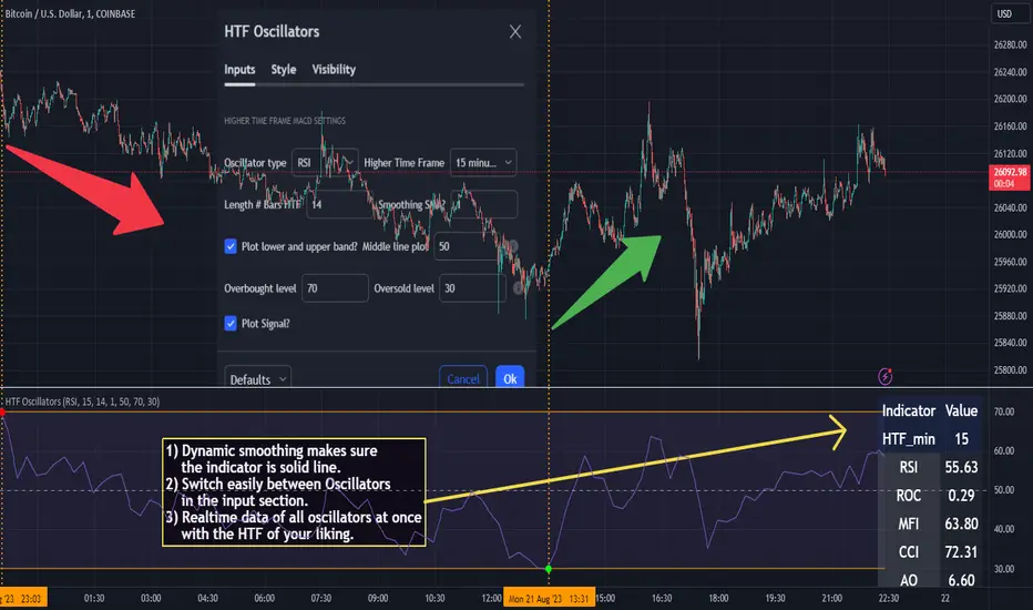
HTF Oscillators RSI/ROC/MFI/CCI/AO - Dynamic SmoothingThe Interplay of Time Frames: A Balanced View
Navigating the markets often involves interpreting trends from multiple angles. The HTF Oscillators with Dynamic Smoothing indicator enables you to do just that. This tool provides the option to integrate smoothed oscillator readings from Higher Time Frames (HTF) into lower time frame charts, such as a 1-minute chart. By doing so, the indicator offers a balanced viewpoint that bridges the gap between micro and macro perspectives, helping you make informed decisions without losing sight of the broader market context.
Features
Multi-Oscillator Support
Choose from a range of popular oscillators like the Relative Strength Index (RSI), Rate of Change (ROC), Money Flow Index (MFI), Commodity Channel Index (CCI), and Awesome Oscillator (AO). These oscillators are commonly used as foundational building blocks in trading strategy scripts by traders worldwide. Switch effortlessly between them, depending on your trading strategy and requirements. To maintain consistency and a familiar user experience, our script adopts the same visual aesthetics that you'll find in Pine Script indicators on TradingView: a sleek purple line for the oscillator and a transparent band filling. These visual elements are not only pleasing to the eye but also widely appreciated by the trading community.
Dynamic Smoothing
The unique dynamic smoothing feature calculates a smoothing factor based on the ratio of minutes between the Higher Time Frame (HTF) and your current time frame. This provides a sleek and responsive oscillator line that still holds the weight of the longer trend. One of the significant advantages of this feature is user experience; when you change your time frame, the HTF-values in your settings will remain consistent. This ensures that you can easily switch between different time frames without losing the insights provided by your selected HTF.
Visual Aids
Visual cues are an essential part of any trading strategy. The indicator not only plots signals to mark overbought and oversold conditions based on the dynamically smoothed oscillator but also provides you with the flexibility to customize your visual experience. You have the option to toggle on/off the display of these signals depending on your specific needs. Additionally, bands can be displayed at overbought and oversold levels, along with a reference middle line. If you switch between different oscillators (available in the parameter settings), remember to manually adjust the bands in the input settings to ensure signals matches with the type of oscillator to your liking.
User-Friendly Settings
We've grouped related settings together, making it easier for you to find what you're looking for. Adjust the oscillator type, length of bars, smoothing settings, and more with just a few clicks.
Information Table
A standout feature of this indicator is the real-time information table, which displays the values of all selected oscillators based on your specified Higher Time Frame (HTF) settings. This can be particularly useful for traders who depend on multiple indicators for their decision-making process. The data presented in the table is synchronized with the HTF options you've configured in the input settings, allowing for a more efficient and quick scan of values from higher time frames.
Educational Corner: The Power of the Information Table and Customization
The table incorporated into this indicator isn't just eye-candy; it's a practical tool designed to elevate your trading strategy. It dynamically displays real-time values of various oscillators for the HTF you've chosen. This is an exemplary use of TradingView's scripting capabilities to blend multiple indicators into a single visual panel, streamlining your analysis and decision-making process.
But here's the best part: You're not limited to what we've created. With some basic understanding of TradingView's scripting language, Pine Script, you can easily adapt this table to include different indicators that suit your unique trading style. The logic in the script is modular and can serve as a foundation for your own customized trading dashboard. So, go ahead, get creative and explore new combinations of indicators that will help you excel in your trading endeavors!
You no longer have to toggle between different charts or indicators to get the information you need; it's all there in one neatly organized table. We encourage you to tap into this feature and make it your own, empowering your trading like never before.
By doing so, you not only gain a more comprehensive toolset, but you also engage more deeply with your trading strategy, understanding its nuances and, ultimately, making more informed decisions.
Conclusion
The HTF Oscillators with Dynamic Smoothing is a versatile and powerful tool that brings together the best of both worlds: the perspective of higher time frames and the granularity of shorter ones. Its feature-rich setting options and real-time information table make it a potential useful addition to your trading toolkit.
Remember, while this indicator offers a comprehensive and smarter way to look at the markets, it is not a foolproof method for predicting market movements. Always use it in conjunction with other analysis methods and risk management strategies.
Statistics: High & Low timings of custom session; 1yr historyGet statistics of the Session High and Session Low timings for any custom session; based on around 1yr of data.
//Purpose:
-To get data on the 'time of day' tendencies of an asset.
-Narrow in on a custom defined session and get statistics on that session.
//Notes:
-Input times are always in New York time (but changing the timezone after setting WILL adust both table stats and background highlight correctly.
-For particularly long sessions, make sure text size is set to 'tiny' (very long vertical table), or adjust table to display horizontally.
-You'll notice most assets show higher readings around NY equities open (9:30am NY time). Other assets will have 'hot-spots' at other times too.
-Timings represent the beginning of a 15m candle. i.e. reading for 15:45 represents a high occurring between 15:45 and 1600.
-Premium users should get 20k bars => around 1year's worth of data on a 15minute chart. Days of history is displayed in the top left corner of the table.
//Limitations
-only designed and working on 15minute timeframe (to gather a full year of meaningful/comparable % stats, need 15minute 'buckets' of time.
-sessions cannot cross through midnight, or start at midnight (00:15 is ok). 00:15 >> 23:45 is the max session length. On BTC, same applies but 01:00 instead of midnight (all in NY time).
-if your session crosses through 'dead time' (e.g. 17:00-18:00 S&P NY time); table will correctly omit these non-existent candles, but it will add on the missing hour before the start time.
//Cautionary note:
-Since markets are not uncommonly in a trending state when your defined session starts or ends, the high/low timings % readings for start and end of session may be misleadingly high. Try to look for unusually high readings that are not at the start/end of your session.
Wheat (ZW1!) 15min chart; Table displayed vertically:
Nasdaq (NQ1!) 15m chart; Table displayed horizontally and with smaller text to view a very long custom session:

RSI Screener and Divergence [5ema]
Displayed on the RSI chart according to a custom timeframe.
Displays the RSI tracking table of various timeframes.
Identify normal divergence, hidden divergence on RSI chat.
Show buy and sell signals (strong, weak) on the board.
Send notifications when RSI has a buy or sell signal.
-----
I reused some functions, made by (i believe that):
©paaax : The table position function.
@everget : The RSI divergence function.
@QuantNomad : The function calculated value and array to show on table for input symbols.
I have commented in my code. Thanks so much!
-----
How it works:
1. Input :
input.int length of RSI => calculate RSI.
input.int upper/lower => checking RSI overbought/oversold.
input.int right bars / left bars => returns price of the pivot low & high point => checking divergence.
input.int range upper / lower bars => compare the low & high point => checking divergence.
input.timeframe => request.security another time frame.
input.string table position => display screener table.
2. Input bool:
plot RSI on chart.
Plot Regular Bullish divergence .
Regular Bearish divergence.
Hidden Bullish divergence .
Hidden Bearish divergence.
3. Basic calculated:
Make function for RSI , pivot low & high point of RSI and price.
Request.security that function for earch time frame.
Result RSI, Divergence.
4. Condition of signal:
Buy condition:
RSI oversold (1)
Bullish divergence (2).
=> Buy if (1) and (2), review buy (1) or (2).
Sell condition:
RSI overbought (3).
Bearish divergence (4).
=> Sell if (3) and (4), review sell (3) or (4).
5. Table screener:
Time frame.
RSI (green - oversold, red - overbought)
Divergence (⬈⬈ - regular bullish , ⬊⬊ regular bearish , ⬊ - hidden bullish , ⬈ - hidden bearish ).
Signal (🟢 - Buy, 🔴 - sell, green 〇 - review buy, red 〇 - review sell)
----
This indicator is for reference only, you need your own method and strategy.
If you have any questions, please let me know in the comments.

Peer Performance - NIFTY36STOCKSI have created a peer performance dashboard for:
36 stocks from:
5 sectors of Nifty 100
This kind of dashboard is very useful for traders when they are planing to trade in a stocks and like to see how that is stocks is performing against other stocks in the same sector . Picking outperforming stocks will always give outstanding results when market starts moving. os having view on teh complete sector will always be good for traders before picking a specific stock.
Sectors covered in this indicators are:
Indian Auto Sector
Banking Sector
Oil, Gas and Energy Stocks
Cement Sector
Technology Sector
It will help traders reviewing performance ( stock return in last 1 year) of group of stocks from a particular sector .
Basically 5 functions are used to plot this dashboard
using "if " function to shortlist the stocks and the sector it belongs to.
tablo function to plot a table with specific parameters like number of row and columns, color of the frame of table
Getting yearly return into a series of variables using "request.security" function
str.tostring function is used to convert yearly return into a series of text so that it can inserted into the table cell.
finally plotting all the text and yearly return values using table.cell function

MLExtensionsLibrary "MLExtensions"
normalizeDeriv(src, quadraticMeanLength)
Returns the smoothed hyperbolic tangent of the input series.
Parameters:
src : The input series (i.e., the first-order derivative for price).
quadraticMeanLength : The length of the quadratic mean (RMS).
Returns: nDeriv The normalized derivative of the input series.
normalize(src, min, max)
Rescales a source value with an unbounded range to a target range.
Parameters:
src : The input series
min : The minimum value of the unbounded range
max : The maximum value of the unbounded range
Returns: The normalized series
rescale(src, oldMin, oldMax, newMin, newMax)
Rescales a source value with a bounded range to anther bounded range
Parameters:
src : The input series
oldMin : The minimum value of the range to rescale from
oldMax : The maximum value of the range to rescale from
newMin : The minimum value of the range to rescale to
newMax : The maximum value of the range to rescale to
Returns: The rescaled series
color_green(prediction)
Assigns varying shades of the color green based on the KNN classification
Parameters:
prediction : Value (int|float) of the prediction
Returns: color
color_red(prediction)
Assigns varying shades of the color red based on the KNN classification
Parameters:
prediction : Value of the prediction
Returns: color
tanh(src)
Returns the the hyperbolic tangent of the input series. The sigmoid-like hyperbolic tangent function is used to compress the input to a value between -1 and 1.
Parameters:
src : The input series (i.e., the normalized derivative).
Returns: tanh The hyperbolic tangent of the input series.
dualPoleFilter(src, lookback)
Returns the smoothed hyperbolic tangent of the input series.
Parameters:
src : The input series (i.e., the hyperbolic tangent).
lookback : The lookback window for the smoothing.
Returns: filter The smoothed hyperbolic tangent of the input series.
tanhTransform(src, smoothingFrequency, quadraticMeanLength)
Returns the tanh transform of the input series.
Parameters:
src : The input series (i.e., the result of the tanh calculation).
smoothingFrequency
quadraticMeanLength
Returns: signal The smoothed hyperbolic tangent transform of the input series.
n_rsi(src, n1, n2)
Returns the normalized RSI ideal for use in ML algorithms.
Parameters:
src : The input series (i.e., the result of the RSI calculation).
n1 : The length of the RSI.
n2 : The smoothing length of the RSI.
Returns: signal The normalized RSI.
n_cci(src, n1, n2)
Returns the normalized CCI ideal for use in ML algorithms.
Parameters:
src : The input series (i.e., the result of the CCI calculation).
n1 : The length of the CCI.
n2 : The smoothing length of the CCI.
Returns: signal The normalized CCI.
n_wt(src, n1, n2)
Returns the normalized WaveTrend Classic series ideal for use in ML algorithms.
Parameters:
src : The input series (i.e., the result of the WaveTrend Classic calculation).
n1
n2
Returns: signal The normalized WaveTrend Classic series.
n_adx(highSrc, lowSrc, closeSrc, n1)
Returns the normalized ADX ideal for use in ML algorithms.
Parameters:
highSrc : The input series for the high price.
lowSrc : The input series for the low price.
closeSrc : The input series for the close price.
n1 : The length of the ADX.
regime_filter(src, threshold, useRegimeFilter)
Parameters:
src
threshold
useRegimeFilter
filter_adx(src, length, adxThreshold, useAdxFilter)
filter_adx
Parameters:
src : The source series.
length : The length of the ADX.
adxThreshold : The ADX threshold.
useAdxFilter : Whether to use the ADX filter.
Returns: The ADX.
filter_volatility(minLength, maxLength, useVolatilityFilter)
filter_volatility
Parameters:
minLength : The minimum length of the ATR.
maxLength : The maximum length of the ATR.
useVolatilityFilter : Whether to use the volatility filter.
Returns: Boolean indicating whether or not to let the signal pass through the filter.
backtest(high, low, open, startLongTrade, endLongTrade, startShortTrade, endShortTrade, isStopLossHit, maxBarsBackIndex, thisBarIndex)
Performs a basic backtest using the specified parameters and conditions.
Parameters:
high : The input series for the high price.
low : The input series for the low price.
open : The input series for the open price.
startLongTrade : The series of conditions that indicate the start of a long trade.`
endLongTrade : The series of conditions that indicate the end of a long trade.
startShortTrade : The series of conditions that indicate the start of a short trade.
endShortTrade : The series of conditions that indicate the end of a short trade.
isStopLossHit : The stop loss hit indicator.
maxBarsBackIndex : The maximum number of bars to go back in the backtest.
thisBarIndex : The current bar index.
Returns: A tuple containing backtest values
init_table()
init_table()
Returns: tbl The backtest results.
update_table(tbl, tradeStatsHeader, totalTrades, totalWins, totalLosses, winLossRatio, winrate, stopLosses)
update_table(tbl, tradeStats)
Parameters:
tbl : The backtest results table.
tradeStatsHeader : The trade stats header.
totalTrades : The total number of trades.
totalWins : The total number of wins.
totalLosses : The total number of losses.
winLossRatio : The win loss ratio.
winrate : The winrate.
stopLosses : The total number of stop losses.
Returns: Updated backtest results table.

SUPER MULTI MOVING AVERAGE [Gabbo]📈 Moving Average Indicator Update - Version 2
🔹 New Features and Improvements:
1️⃣ Enhanced MA Selection for Table Lines:
Previously, the indicator did not allow users to choose a different Moving Average type for the table lines. Now, you can select the MA type for the table.
2️⃣ New Table Text Customization Inputs:
Added inputs to choose the table text color and size for a more personalized display.
3️⃣ Improved Input Visibility and Organization:
We’ve reorganized the inputs so that the most commonly used options are now placed at the beginning for quicker and more convenient configuration.
4️⃣ Bug Fixes and Code Improvements:
Minor bugs have been fixed, and the code has been optimized for improved stability and performance. The code is now cleaner and fully functional in version 6.
5️⃣ Cometreon Public Library Integration:
To lighten the code and improve modularity, we’ve integrated the Cometreon public library. This makes the code more efficient and reduces the need to duplicate common functions.
☄️ With this update, the Moving Average indicator becomes even more versatile and user-friendly, offering a refined table interface and enhanced customization options!

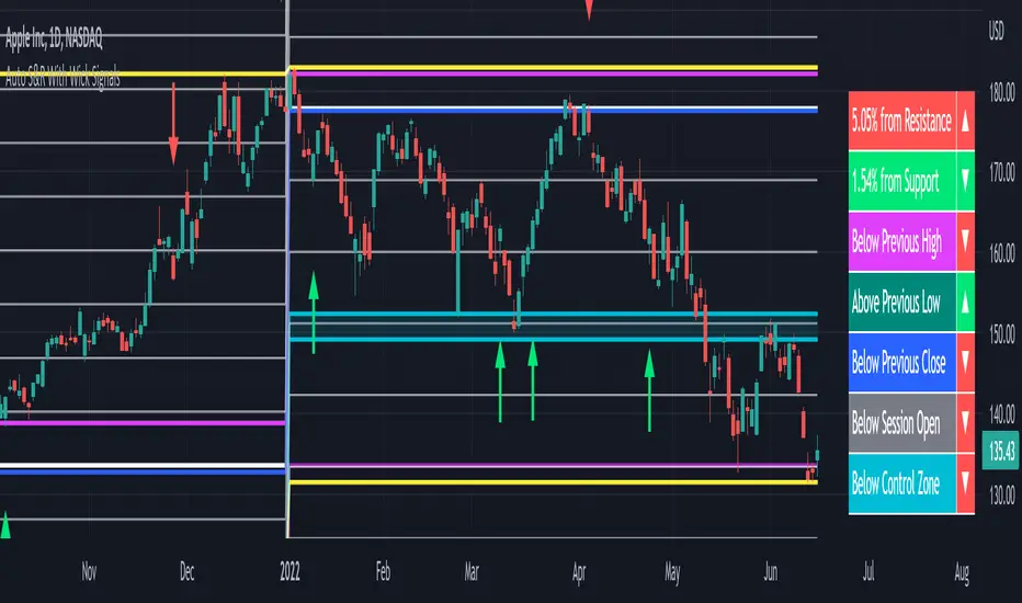
Auto Support & Resistance With Wick Signals & Percentage GapsThis auto support and resistance indicator uses percentage deviations from the previous session close to calculate levels. It provides arrows as signals when it detects 2 wicks in the last 5 bars from a support or resistance level. Includes alerts for price crossing any level as well as real time percentage gaps from current price to the next closest support and resistance level. You also have the option to set up to 3 major levels of your own for any levels that are very important on longer timeframes that you want included. Those will show on the chart as well as within your percentage gap table with color coded background. All features can be customized or turned off to suit your preferences.
SOURCE
This indicator uses the previous session close as a source by default but can be adjusted to use the previous session high or the previous session low. I find the close setting to provide the most accurate levels.
SESSION
The default setting for the previous session used is the daily session but can be adjusted to use the daily, weekly, monthly, quarterly or yearly session. Use longer sessions when looking at longer time frame charts.
SIGNALS
The signals by default are set to only show an arrow if there have been 2 bullish or bearish wicks off of a support or resistance level in the last 5 bars. This can be changed to one bullish wick off of support and one bearish wick off of resistance or it can be set to give a signal anytime a bar crosses a support or resistance level. This can be controlled in the indicator settings.
PERCENTAGE DEVIATION LEVELS
The default percentage deviation is set to 1% but can and should be adjusted according to whatever ticker you are using. For example use .25% or .5% when looking at forex intraday charts since they are not as volatile as other markets. For leveraged etfs used 1% multiplied by the leverage on the etf, so for SQQQ use 3% as it is a 3x leveraged etf. When looking at longer timeframes or highly volatile charts, set the percentage deviation to 2%, 5%, 10%, etc.
LINE COLORS
The color of the lines will change from red to green depending on if the price is above or below that level. You can customize these colors in the settings.
MAJOR LEVELS
If you have major levels of support and resistance from longer timeframes and your own charting, you can add up to 3 major levels that will show on the chart as well as show the percentage gaps in the table. The label for each major level will be colored to match the color of the line on the chart individually.
PERCENTAGE GAP TABLE
The gap table will update live with percentages to go from current price to the next closest support and resistance levels so you don’t have to calculate them manually. The position of the percentage gap table can also be changed within the indicator settings.
TURN FEATURES ON/OFF
There are 3 toggle switches so you can easily turn on or off certain features such as: the support and resistance lines, the percentage gaps table and the arrow signals.
LINE WIDTHS
You can also set the line width of all levels and the line width of the starting level within the indicator settings.
***MARKETS***
This indicator can be used as a signal on all markets, including stocks, crypto, futures and forex.
***TIMEFRAMES***
This automatic support and resistance indicator can be used on all timeframes as long as there is enough data for the session used.
***TIPS***
Try using numerous indicators of ours on your chart so you can instantly see the bullish or bearish trend of multiple indicators in real time without having to analyze the data. Some of our favorites are our Volume Spike Scanner, Volume Profile, Momentum and Trend Friend in combination with this auto support and resistance indicator. They all have real time Bullish and Bearish labels as well so you can immediately understand each indicator's trend.
Script Title: FX Exchange Simulator: Two Investors (Gain vs. LosDescriptionOverviewThis educational tool is designed to help traders and beginners understand the mechanics of currency exchange rates in the EUR/USD pair. It simulates two distinct investor scenarios based on the highest and lowest prices over a user-defined period (default: 100 bars).The Two ScenariosThe script compares how the direction of exchange and the timing of the trade impact final purchasing power:Investor 1 (Starting with USD - The Strategic Entry):At the Low: Converts $1,000 USD into EUR by dividing the amount by the exchange rate.At the High: Converts those EUR back into USD by multiplying.Result: Demonstrates how buying a currency when it is "cheap" (at the low) increases your total capital in dollars.Investor 2 (Starting with EUR - The Timing Error):At the Low: Panics and converts 1,000€ into USD by multiplying.At the High: Tries to recover the 1,000€ by dividing the USD back at a higher rate.Result: Demonstrates how selling a currency when it is "cheap" and buying it back when it is "expensive" leads to a significant loss of purchasing power.FeaturesDynamic Historical Analysis: Automatically finds the highest and lowest points within the selected lookback period.Step-by-Step Calculation Table: A clean, top-centered table showing the initial amount, the exchange process, the final total, and the ROI (Return on Investment) percentage.Visual Annotations: Labels on the chart pinpoint exactly where the "Minimum" and "Maximum" occurred to provide visual context for the trade simulation.Fully Customizable: Users can adjust the initial capital amount and the lookback period via the settings menu.Mathematics Behind the ScriptThe script uses the following formulas for the calculations:Profit Scenario (USD to EUR):$$\text{Total USD} = \left( \frac{\text{Initial USD}}{\text{Price}_{min}} \right) \times \text{Price}_{max}$$Loss Scenario (EUR to USD):$$\text{Total EUR} = \left( \text{Initial EUR} \times \text{Price}_{min} \right) / \text{Price}_{max}$$InstructionsAdd the script to your chart (best used on EUR/USD).Look at the labels to see where the period extremes are.Check the table at the top to see the financial outcome of both investors.Use the "Settings" to change the initial amount or the bar period to test different market cycles.DisclaimerThis script is for educational purposes only. It is intended to illustrate currency exchange mechanics and does not constitute financial advice.

Inside Bar False Breakout (IBFB)The Inside Bar False Breakout (IBFB) is a price action tool that identifies high-probability reversal setups by detecting false breakouts from inside bar patterns. This strategy is widely used by traders to catch market traps and potential trend reversals.
What is an Inside Bar False Breakout?
An Inside Bar occurs when a candle's high and low are completely contained within the previous candle's range. A False Breakout happens when price initially breaks above or below this range but then closes back inside it, indicating a failed breakout and potential reversal.
How It Works
Step 1: Inside Bar Detection
Identifies candles where high < previous high AND low > previous low
Marks consolidation zones where market indecision occurs
Step 2: False Breakout Recognition
Bullish IBFB: Price breaks below the inside bar's low but closes back inside the range (bullish reversal signal)
Bearish IBFB: Price breaks above the inside bar's high but closes back inside the range (bearish reversal signal)
Step 3: Signal Confirmation
Applies a cooldown period (default 5 bars) to filter out noise and prevent signal clustering
Key Features
✅ Visual Signals
Color-coded bars (green for bullish, red for bearish IBFB)
Free-floating arrow markers (⬆ bullish, ⬇ bearish) without label boxes
Clean, minimalist design that doesn't clutter your chart
✅ Signal History Table
Displays the last 5 IBFB signals in real-time
Shows date/time, signal type, and price level
Color-coded for quick reference
✅ Customizable Settings
Enable/disable bullish or bearish signals independently
Adjustable cooldown period (1-100 bars) to control signal frequency
Customizable colors for both signal types
Toggle arrows and history table on/off
✅ Alert System
Built-in alert conditions for both bullish and bearish IBFB patterns
Fires once per bar close to avoid false alarms
Perfect for automated trading or notifications
✅ Universal Compatibility
Works on ANY timeframe (1m to 1M)
Lightweight and efficient - won't slow down your charts
No repainting - signals appear only on confirmed bar close
Best Use Cases
a.Scalping & Day Trading: Catch intraday reversals on lower timeframes (5m, 15m)
b.Swing Trading: Identify multi-day reversal patterns on higher timeframes (4H, D)
c.Trend Confirmation: Combine with trend indicators to filter trades in the direction of the main trend
d.Support/Resistance: Works exceptionally well near key S/R levels where false breakouts are common
Trading Tips
Confluence is Key: Combine IBFB signals with support/resistance zones, trendlines, or Fibonacci levels
Volume Matters: Look for decreasing volume on the false breakout for stronger confirmation
Risk Management: Place stop-loss just beyond the false breakout wick; target the opposite side of the inside bar range
Trend Alignment: Best results when trading in the direction of the higher timeframe trend
Cooldown Period: Increase the cooldown on lower timeframes to reduce noise; decrease on higher timeframes for more signals
Settings Explained
Signal Settings
Show Bullish/Bearish IBFB: Toggle each signal type independently
Cooldown Period: Minimum bars between signals (prevents over-trading)
Visual Settings
Show Arrows: Display ⬆⬇ markers on chart
Show Last 5 Signals Table: Display signal history panel
Bullish/Bearish Color: Customize signal colors
Alert Settings
Enable Alerts: Turn on/off automatic alert notifications
Why This Indicator?
Unlike many indicators that lag behind price action, the IBFB indicator identifies real-time market manipulation and traps. False breakouts often indicate:
Stop-loss hunting by institutional traders
Exhaustion of buying/selling pressure
Potential trend reversals or strong counter-moves
This makes it an excellent tool for contrarian traders and those looking to fade false moves.
Performance Notes
Signals confirm at bar close (no repainting)
Optimized for speed and efficiency
Works alongside other indicators without conflicts
Suitable for manual and automated trading strategies
Suitable for any instrument & market
Disclaimer: This indicator is for educational purposes only. Always practice proper risk management and combine with your own analysis before making trading decisions. Happy trading.

Entry ChecklistEntry Checklist
A comprehensive multi-factor analysis tool for stock and crypto entry decisions, combining fundamental, technical, and market sentiment indicators in a dynamic table display.
🎯 Overview
This advanced Pine Script indicator provides traders and investors with a systematic checklist for evaluating potential entry points. It consolidates critical market data into a clean, color-coded table that adapts based on asset type and data availability.
📊 Key Features
Market Context Analysis:
Seasonality: Historical S&P 500 monthly return patterns with strength/weakness labels
Market Breadth (S5TH): Percentage of S&P 500 stocks above their 50-day moving average
Fear/Greed Index (VIX): Market sentiment indicator with threshold-based color coding
Fundamental Analysis (Stocks Only):
Earnings Dates: Upcoming earnings announcement tracking with 14-day warning
Growth Metrics: Year-over-year sales and EPS growth rates
Acceleration: Quarter-over-quarter growth acceleration analysis
Sector & Industry Analysis:
Sector Relative Strength: 20-day performance vs SPY benchmark
Industry Relative Strength: Granular industry ETF performance comparison
120+ Industry ETF Mappings: Comprehensive sector and industry classifications
Technical Analysis:
IBD-Style RS Rating: Multi-timeframe relative strength scoring (1-99 scale)
RS vs SPX: Stock performance relative to S&P 500
RS vs Sector: Performance relative to sector ETF
RS vs Industry: Performance relative to industry ETF
🎨 Visual Design
Dynamic Table: Bottom-right overlay with professional dark theme
Color-Coded Signals: Green (bullish), red (bearish), neutral (white)

SEPA Sell Signal IndicatorSEPA Sell Signal Indicator - Documentation
Overview
A comprehensive exit signal indicator designed to work alongside the main SEPA (Stage, EMA, Price Action) indicator. It detects entry points via SEPA base breakouts and provides intelligent sell signals to protect profits and limit losses.
Core Features
Entry Detection
Automatically detects SEPA base breakout patterns
Tracks entry price and calculates swing low reference
Monitors position status (LONG/FLAT)
5 Sell Triggers
Price < EMA50 (Technical weakness)
Protected by EMA10 system (see below)
Trend Broken (Price < EMA150 AND EMA200)
Major trend reversal signal
Not protected - always fires
EMA Cross (EMA50 < EMA150)
Death cross indicating momentum shift
Not protected - always fires
Swing Low Broken (Price < Previous Swing Low)
Hard stop loss trigger
Lookback period: 10 bars (adjustable 5-50)
Not protected - always fires
Relative Strength Negative (RS vs NIFTY500 < 0)
Stock underperforming benchmark index
Based on 21-period EMA comparison
Not protected - always fires
EMA10 Protection System (Refinement Feature)
Purpose
Prevents premature exits during healthy pullbacks in strong uptrends.
Protection Criteria (All must be true)
✅ Stock in uptrend (EMA50 > EMA150 > EMA200)
✅ Price above EMA10
✅ Price above EMA50
✅ Only protects Condition 1 (Price < EMA50)
Two-Stage Warning System
Stage 1: Yellow "CAUTION" Signal
Appears when Condition 1 triggers but protection is active
Grace period begins (default: 5 bars)
Allows time for price to recover
Stage 2: Red "SELL" Signal
Fires when ANY of these occur:
Warning timer expires (5/5 bars)
Price drops below EMA10
Price drops below EMA50
Uptrend ends
Any other sell condition (2-5) triggers
Settings
Enable EMA10 Protection: ON/OFF toggle (default: ON)
Protection Time Limit: 1-20 bars (default: 5)
Visual Elements
Chart Signals
🔴 Red Triangle (SELL): Confirmed sell signal - exit position
🟡 Yellow Circle (CAUTION): Warning - monitor closely
🟢 Green Background Tint: Currently in position
Information Tables
Top Right - Sell Conditions Table
Shows real-time status of all 5 conditions
✓ (Green) = Condition NOT met (safe)
✓ (Red) = Condition met (danger)
⚠ (Yellow) = Warning active (monitoring)
Displays EMA10 protection status (ON/OFF)
Shows warning timer (e.g., "3/5")
Bottom Right - Position Details (when in position)
Entry price
Swing low level
Relative strength value (color-coded)
Current P&L percentage
Bottom Right - Status (when flat)
Shows "NO POSITION"
Indicates waiting for "BASE BREAKOUT"
Alert System
Entry Signal: SEPA base breakout detected
Warning Alert: Caution - price below EMA50 but protected
EMA50 Break: Sell confirmed after protection expires
Trend Break: Major reversal - exit immediately
EMA Cross: Death cross - exit immediately
Swing Low Break: Hard stop - exit immediately
RS Negative: Underperformance - exit immediately
Configuration Parameters
ParameterDefaultRangeDescriptionEMA 10101-50Fast moving average for protectionEMA 50501-200Primary trend indicatorEMA 1501501-300Medium-term trendEMA 2002001-500Long-term trendSwing Low Lookback105-50Bars to find previous swing lowRS EMA215-50Period for relative strength calcBenchmarkCNX500-Index for RS comparisonProtection Time Limit51-20Max bars for warning stateTable Text Size1 (Small)0-40=Tiny, 4=HugeEMA10 ProtectionONON/OFFEnable/disable protection
Trading Workflow
Entry: Indicator detects SEPA base breakout
Monitoring: Track 5 sell conditions in real-time
Warning: Yellow CAUTION if minor weakness (Condition 1 only)
Grace Period: 5 bars to recover or confirm breakdown
Exit: Red SELL signal when conditions confirm weakness
Reset: Returns to flat, waits for next base breakout
Key Advantages
✅ Selective Protection: Only protects shallow pullbacks, not real breakdowns
✅ Time-Limited: Won't delay exits indefinitely (5-bar max)
✅ Multi-Layered: 5 independent sell conditions
✅ Visual Clarity: Color-coded signals and comprehensive tables
✅ Customizable: All parameters adjustable for your style
✅ Alert System: Never miss a critical signal
Philosophy
The indicator balances two competing goals:
Stay in winning trades during healthy pullbacks
Exit quickly when trends genuinely reverse
The refined EMA10 protection system achieves this by giving breathing room for minor dips while ensuring swift exits on confirmed weakness.

Hap Mum Formasyonu - Candlestick PatternsThis indicator is a comprehensive tool that automatically scans for popular Candlestick Patterns on symbols you select and displays the results in a table on your screen.
Unlike standard scanners, this script allows you to create 10 Different Custom Watchlists. You can add up to 20 symbols to each list and switch between lists via the settings menu to see instant scanning results.
🚀 Key Features
10 Custom Lists: Organize your portfolio into groups (e.g., Indices, Crypto, Forex). Each list holds 20 symbols.
Trend Filter: Patterns are validated based on the trend direction, not just the candle shape. Bullish patterns are searched in downtrends, and Bearish patterns in uptrends.
Option 1: Is Price above/below SMA 50?
Option 2: Price relative to SMA 50 & SMA 200 alignment.
Visual Table: Bullish signals are shown in the Green box, Bearish signals in the Red box.
Flexible Settings: You can toggle specific patterns on/off and change the trend detection method.
📊 Supported Patterns & Legend
Abbreviations used in the dashboard:
Bullish Signals:
DD: Dragonfly Doji
H: Hammer
IH: Inverted Hammer
EB: Engulfing Bullish
MS: Morning Star
MDS: Morning Doji Star
P: Piercing Line
HB: Harami Bullish
TWS: Three White Soldiers
Bearish Signals:
GD: Gravestone Doji
HM: Hanging Man
SS: Shooting Star
EB: Engulfing Bearish
ES: Evening Star
EDS: Evening Doji Star
HB: Harami Bearish
TBC: Three Black Crows
DCC: Dark Cloud Cover
🛠 How to Use?
Add the indicator to your chart.
Open Settings.
Select a list from "Which List Do You Want to Scan?" (e.g., List 1).
Enter your ticker symbols into the corresponding group fields below (LIST 1, LIST 2...).
Click OK, and the table will update with the signals.
Disclaimer: This tool is for educational purposes only. Candlestick patterns do not guarantee future market movements. Always manage your risk.

#BLTA - CARE 7891🔷 #BLTA - CARE 7891: Ny session toolkit + Risk box + Confirmed levels + Asia box + Structure + Imbalances
Description:
#BLTA - CARE 7891 is an overlay toolkit 🧭🛠️ built for structured discretionary trading preparation. Its main purpose is to keep your chart reading and pre-trade planning in one place by combining time context, confirmed reference levels, liquidity framing, manual risk sizing, and context overlays (structure + imbalances).
🚫 This script is an indicator, not a strategy. It does not place orders.
🧩 Why these modules are combined (and how they work together)
This is not a “mashup for the sake of mixing”. Each module supports a specific step of a practical workflow:
🕒 Time context (new york session mapping)
Background highlights mark precise NY-time windows (day division at 17:00, london blocks, and new york blocks).
This provides the timing framework for when you typically scan, plan, or execute.
📰📅 Confirmed reference levels (previous day/week highs & lows)
Instead of plotting live extremes, this script confirms levels at defined boundaries:
Trading day: 17:00 → 17:00 NY
Weekly boundary: Sunday 17:00 NY
Lines start exactly at the candle where the high/low occurred and extend forward.
Optional “stop on hit” 🧊 freezes a level once price touches it, keeping the chart clean and realistic for forward analysis.
🈵 Asian range liquidity box (session that can cross midnight)
A dedicated Asian range container tracks high/low and an optional 50% midline.
It uses NY timestamps and safely handles sessions that cross midnight (storing the correct session date).
This gives you a daily liquidity “frame” often used for sweeps, breaks, and invalidations.
💸 Manual risk planning (trade box + lot sizing + table)
You select Entry (EP) and Stop (SL) directly on the chart using input.price(..., confirm=true) and time anchors.
The script then calculates:
💰 cash at risk from balance and risk %
📏 stop distance in pips (forex-aware pip sizing)
📦 lot size using units-per-lot and account currency inputs
🎯 target price using a reward ratio
It draws a risk box + target box and shows a compact table for quick verification.
🔁 Re-confirm mode (wizard) is included to prevent “stale” anchor points after timeframe changes or when you want a clean reset. While enabled, the risk table is replaced with a step guide and temporary EP/SL markers.
📈 Market structure overlay (1H zigzag projected to any timeframe)
A zigzag swing engine is computed on 1H via request.security() and projected onto the current chart.
Opacity is automatically reduced on non-1H charts so it stays contextual, not dominant.
Optional live extension of the last leg helps you see the active swing in progress.
📊 Imbalance map (fvg / og / vi) + optional dashboard
The script detects and draws:
🤏 fair value gaps (fvg)
👐 opening gaps (og)
🔎 volume imbalances (vi)
Optional filters allow minimum width by points / % / atr, and each imbalance type can be extended forward.
A dashboard 📱 can summarize bullish/bearish frequency and fill rates for context review.
✅ Quick start (recommended order)
Turn on 🕒 session visualization to align with NY timing.
Enable 📰 pdh/pdl and 📅 weekly highs/lows to map confirmed reference liquidity.
Use 🈵 the asian range box to frame the early-session liquidity container.
Plan your trade with 💸 risk module (pick EP/SL, verify pips + lots + target).
Add 📈 zigzag structure and 📊 imbalances only as supporting context.
⚠️ Notes & limitations
This tool is for planning and chart reading, not automated execution.
Lot sizing is an estimate based on your inputs; always confirm broker contract specs.
Some modules draw many objects (boxes/lines/tables) 🧱, which may slow very small timeframes.
