NQ B3X-S1.5X cash by BellevueFXNQ B3X-S1.5X Cash by BellevueFX
Precision Breakout Engine for Nasdaq Futures (NQ)
The NQ B3X-S1.5X Cash indicator by BellevueFX is an advanced price-action and volatility-driven breakout system designed for short-term scalpers, intraday traders, and algorithmic strategy builders focused on Nasdaq (NQ) or high-volatility assets.
It combines ATR-adaptive trailing logic, EMA structure alignment, and dynamic target generation to highlight institutional momentum shifts and sniper entry zones in real time.
⚙️ Core Features
📈 ATR-Adaptive Trailing Stop:
Automatically adjusts to volatility for accurate dynamic stop levels.
🧠 Smart Sensitivity Control:
Fine-tune responsiveness using the Key Sensitivity parameter — higher values smooth noise, lower values increase reactivity.
🔵 EMA Trend Alignment:
EMA-50 and EMA-200 act as directional filters and structure references.
🧭 Heikin Ashi Option:
Optionally use HA candles for smoother breakout confirmation.
🎯 Dynamic TP/SL Levels:
Automatically draws ENTRY, STOP LOSS, TP1, and TP2 levels for each signal — cleanly synchronized with the current price.
🔔 Built-in Alerts:
Ready-to-use Long and Short alert conditions for automated trade execution or signal notifications.
💡 How It Works
The system continuously measures volatility through ATR(500) and reacts dynamically to price structure:
BUY signal: When price crosses above the trailing baseline and confirms bullish momentum.
SELL signal: When price falls below the baseline and momentum confirms bearish reversal.
Targets: Automatically projected based on swing structure (2× and 4× distance from SL).
⚡ Best Use Cases
Works best on Nasdaq (NQ), but also effective on US30, SPX, and XAUUSD.
Designed for scalping, momentum trading, and breakout confirmations.
Compatible with BellevueFX AI tools and future Profitcosmos automation modules.
🧩 Recommended Settings
Default sensitivity: 9.0
ATR period: 500
Swing lookback: 5
Use on 1-min and 5-min charts for best performance.
🧠 Developer
BellevueFX — a division of Groupe Bellevue Inc.
Focused on precision trading systems, AI-driven analytics, and professional automation tools for active traders.
🔗 Visit www.profitcosmos.com
for strategy packs, tools, and automation updates.
Cari dalam skrip untuk "ai"

Multi-TF FVG Kerze Break AlertHere's a breakdown of the key files:
App.tsx: This is the main component that orchestrates the entire user interface. It manages the application's state, including the input Pine Script, the selected target language, the resulting converted code, and the loading/error states.
services/geminiService.ts: This file handles all communication with the Google Gemini API. It takes the Pine Script and the target language, constructs a detailed prompt instructing the AI on how to perform the conversion, sends the request, and processes the response.
components/CodeEditor.tsx: A reusable UI component that provides a styled for both displaying the input Pine Script and the read-only output.
constants.ts: This file centralizes static data. It contains the list of target languages for the dropdown menu and the default Pine Script code that loads when the application first starts.
index.html & index.tsx: These are the standard entry points for the React application, responsible for setting up the web page and mounting the main App component.
In essence, the application provides a user-friendly interface for developers to convert financial trading algorithms written in TradingView's Pine Script into other popular programming languages, leveraging the power of the Gemini AI model to perform the translation.

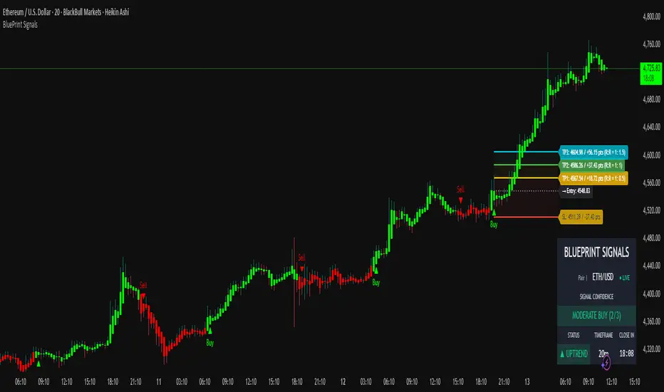
Blueprint Signals ProBlueprint Signals Pro is an advanced, all-in-one trading indicator designed for TradingView, built to provide high-quality buy/sell signals across various markets including cryptocurrencies, U.S. stocks, Indian indices, forex, and more. 📈 It leverages a proprietary ATR-based trailing stop mechanism combined with AI-optimized profiles for different trading styles (scalping, intraday, swing, and position trading) to generate reliable signals on bar close.
Key Features:
📊 Market Optimization: Tailored options for specific markets like Cryptocurrency (high volatility, 24/7 trading), U.S. Stocks (regulated exchanges, standard hours), Indian Indices (local dynamics like NIFTY), and Forex (high liquidity, global influences) to customize parameters and enhance signal accuracy.
🎨 Theme & Palette Customization: Supports dark/light chart themes with multiple color palettes for visual appeal.
🤖 Trading Profiles: Pre-built AI profiles like "Edge Signal", "Flash Signal", "Trend Rider", etc., tailored to your timeframe and style.
🔍 Signal Filters: Bullish/Bearish modes to focus on one-sided signals, with adjustable candle opacity.
🛡️ Support/Resistance Zones: Dynamic S/R levels with auto-adjusting lookback and wick warning markers for potential reversals.
⚠️ Swing Pattern Failure (SPF): Detects failure patterns with volume and wick filters for early reversal alerts.
🚨 Warnings: Proximity and wick-touch alerts on the trailing stop to signal momentum loss or trend challenges.
💡 Premium/Discount Zones: Neon-style P&D zones with glow effects to identify overvalued/undervalued areas.
📉 Custom Moving Averages: Up to 3 configurable MAs (EMA/SMA/WMA/HMA) with theme-based colors.
⚙️ Core Parameters: Manual/auto-tuning for scaling factor, period, min move filter, and anti-chop sensitivity.
⭐ Confidence Rating: Scores signals (Weak/Moderate/Strong) based on trend, S/R proximity, and volume.
🎯 SL/TP Levels: Displays stop loss (ATR trail, swing, or fixed ATR) and multiple take profits with R:R ratios, extendable lines, and zone fills. Additionally, clearly shows captured points/pips (e.g., +50 pts) and potential profit in points/pips/₹ for each level, making risk-reward analysis straightforward and visible on the chart.
🖥️ Display Options: Toggle trailing stop, text on signals, and more.
📅 Dashboard: Multi-timeframe overview with trend intelligence (using ADX), confidence, and candle timer.
🔔 Alerts: Configurable for buy/sell signals with detailed messages.
Usage Guidelines:
Select your market, theme, and trading style from the inputs.
Use on any timeframe; auto-adjusts for optimal performance.
Signals are confirmed on bar close to avoid repainting.
Combine with your risk management; backtest thoroughly.
This indicator is for educational and informational purposes only. Past performance is not indicative of future results. Trade at your own risk. © 2025 Raza | Blueprint Signals. All Rights Reserved.
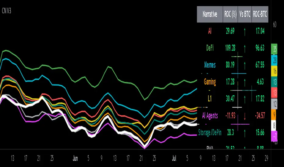
Crypto Narratives: Relative Strength V2Simple Indicator that displays the relative strength of 8 Key narratives against BTC as "Spaghetti" chart. The chart plots an aggregated RSI value for the 5 highest Market Cap cryopto's within each relevant narrative. The chart plots a 14 period SMA RSI for each narrative.
Functionality:
The indicator calculates the average RSI values for the current leading tokens associated with ten different crypto narratives:
- AI (Artificial Intelligence)
- DeFi (Decentralized Finance)
- Memes
- Gaming
- Level 1 (Layer 1 Protocols)
- AI Agents
- Storage/DePin
- RWA (Real-World Assets)
- BTC
Usage Notes:
The 5 crypto coins should be regularly checked and updated (in the script) by overtyping the current values from Rows 24 - 92 to ensure that you are using the up to date list of highest marketcap coins (or coins of your choosing).
The 14 period SMA can be changed in the indicator settings.
The indicator resets every 24 hours and is set to UTC+10. This can be changed by editing the script line 19 and changing the value of "resetHour = 1" to whatever value works for your timezone.
There is also a Rate of Change table that details the % rate of change of each narrative against BTC
Horizontal lines have been included to provide an indication of overbought and oversold levels.
The upper and lower horizontal line (overbought and oversold) can be adjusted through the settings.
The line width, and label offset can be customised through the input options.
Alerts can be set to triggered when a narrative's RSI crosses above the overbought level or below the oversold level. The alerts include the narrative name, RSI value, and the RSI level.
Target ScannerThis invite-only indicator implements an advanced Wolfe Wave pattern recognition system specifically designed for Borsa Istanbul (BIST) stock screening across multiple timeframes and mathematical ratio calculations.
**Core Technical Framework:**
The indicator employs sophisticated mathematical calculations across 10 distinct timeframes (377, 233, 144, 89, 55, 34, 21, 13, 8, 5 periods) using Elliott Wave ratio theory combined with algorithmic pattern detection. Unlike standard scanning tools that rely on basic technical indicators, this system uses quantitative Wolfe Wave analysis to identify precise entry and exit points across 560+ BIST stocks simultaneously.
**Key Features:**
• **Multi-Stock Scanning:** Simultaneously analyzes 40 stocks per list across 14 different BIST stock lists (560+ total stocks)
• **Advanced Pattern Detection:** Implements Wolfe Wave mathematical validation using 24 different ratio calculation methods including Fibonacci sequences, Elliott Wave ratios, Golden Ratio, Harmonic Patterns, Pi-based calculations, volatility-based dynamic ratios, and AI-optimized mathematical progressions
• **Real-Time Screening Table:** Displays active signals with current price, signal price, target price, expected profit percentage, and calculated stop-loss levels
• **Reliability Scoring System:** EPA (Entry Point Accuracy) and ETA (Exit Target Accuracy) scoring with historical performance tracking
• **Visual Signal Display:** Comprehensive signal boxes showing profit zones, stop-loss areas, entry levels, and estimated time to target completion
**Mathematical Implementation:**
The core algorithm calculates price relationships using configurable mathematical ratios. For bullish conditions, it identifies entry points when price action meets specific criteria:
- Point validation through ratio analysis between swing highs/lows across multiple timeframes
- Mathematical confirmation using (pv - pf) / (pv - pd) ratio calculations
- Confluence validation across timeframes with dynamic ratio adjustments
- Minimum profit threshold filtering to ensure signal quality
**Originality and Innovation:**
This implementation differs significantly from traditional scanning tools through several key innovations:
1. **Multi-Timeframe Wolfe Wave Detection:** Simultaneous pattern recognition across 10 timeframes rather than single-timeframe analysis
2. **Adaptive Ratio Systems:** 24 different mathematical calculation methods including volatility-based, time-based, momentum-based, and volume-weighted ratio adjustments
3. **BIST-Specific Optimization:** Tailored specifically for Turkish stock market characteristics with 14 pre-configured stock lists
4. **Institutional-Grade Visualization:** Advanced signal boxes with profit/loss zones, multiple entry levels, and time-based target estimation
5. **Real-Time Performance Tracking:** Dynamic EPA/ETA scoring system that tracks historical accuracy and adapts calculations
**Signal Generation Logic:**
The system generates signals when multiple mathematical conditions align:
- Wolfe Wave pattern completion across specified timeframes
- Ratio validation using selected mathematical progression (Fibonacci, Golden Ratio, Elliott Wave, etc.)
- Stop-loss calculation as percentage of target profit (default 0.5%)
- Minimum profit threshold compliance
- Multi-timeframe confluence confirmation
**Risk Management Features:**
• **Configurable Stop-Loss:** Calculated as percentage of target profit with recommended 0.3 setting for 1:3 risk-reward ratio
• **Profit Percentage Display:** Real-time calculation showing expected profit from signal price to target
• **Multiple Entry Levels:** EPA and ETA-based entry points with reliability scoring
• **Time Estimation:** Statistical analysis providing estimated bars/time to target completion
• **Visual Risk Zones:** Color-coded profit (green) and loss (red) areas for clear risk visualization
**Performance Characteristics:**
The indicator is optimized for active screening with frequent signal generation across multiple stocks. It provides both short-term and medium-term opportunities depending on the timeframe producing the signal. The system maintains historical statistics for signal accuracy and target completion timing.
**Technical Requirements:**
Requires understanding of Wolfe Wave pattern theory, Elliott Wave principles, and multi-timeframe analysis concepts. Users should be familiar with BIST market structure and Turkish stock trading mechanics. The indicator demands active monitoring due to the high-frequency nature of multi-stock scanning.
**Market Application:**
Specifically designed for Borsa Istanbul stocks with comprehensive coverage across major sectors. Works effectively in both trending and ranging market conditions due to its adaptive ratio selection and multi-timeframe approach. Best suited for traders focusing on Turkish equity markets with pattern-based strategies.
**Customization Options:**
• **14 Stock Lists:** Pre-configured BIST stock groups for sector-specific analysis
• **24 Ratio Methods:** From conservative Fibonacci to aggressive AI-optimized calculations
• **Quote Pair Integration:** Optional currency pair specification for international analysis
• **Timeframe Flexibility:** Customizable chart timeframe for signal generation
• **Table Positioning:** Multiple display options with size and color customization
• **Alert Integration:** Comprehensive alert system for real-time signal notifications

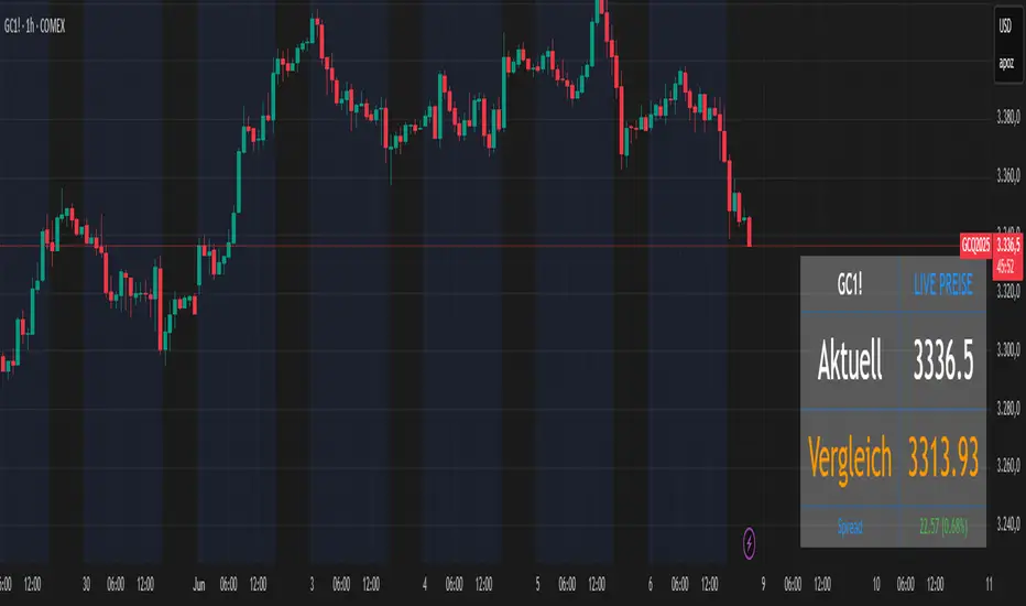
Futures vs CFD Price Display
🎯 Trading the same asset in CFDs and Futures but tired of switching charts to compare prices? This is your indicator!
Stop the constant chart hopping! This live price comparison shows you instantly where the better conditions are.
✨ What you get:
Bidirectional: Works in both Futures AND CFD charts
Live prices: Real-time comparison of both markets
Spread calculation: Automatic difference in points and percentage
Fully customizable: Colors, position, size to your liking
Professional design: Clean display with symbol header
🎯 Perfect for:
Gold traders (Futures vs CFD)
Arbitrage strategies
Spread monitoring
Multi-broker comparisons
⚙️ Customization:
3 sizes (Small/Normal/Large) for all screens
4 positions available
Individual color schemes
Toggle features on/off
💡 Simply enter the symbol and keep both markets in sight!
Notice: "Co-developed with Claude AI (Anthropic) - because even AI needs to pay the server bills! 😄"
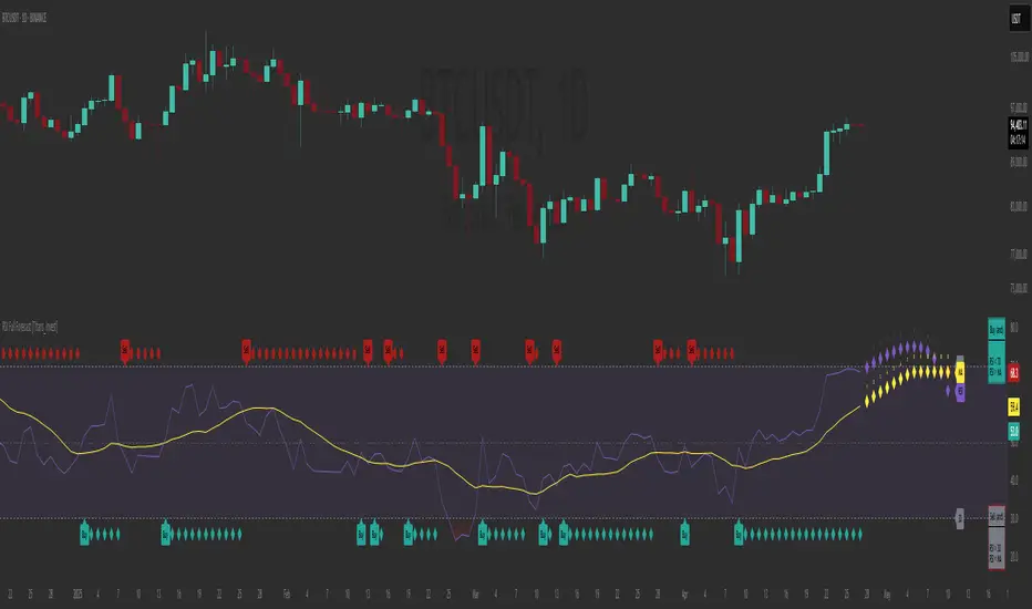
RSI Full Forecast [Titans_Invest]RSI Full Forecast
Get ready to experience the ultimate evolution of RSI-based indicators – the RSI Full Forecast, a boosted and even smarter version of the already powerful: RSI Forecast
Now featuring over 40 additional entry conditions (forecasts), this indicator redefines the way you view the market.
AI-Powered RSI Forecasting:
Using advanced linear regression with the least squares method – a solid foundation for machine learning - the RSI Full Forecast enables you to predict future RSI behavior with impressive accuracy.
But that’s not all: this new version also lets you monitor future crossovers between the RSI and the MA RSI, delivering early and strategic signals that go far beyond traditional analysis.
You’ll be able to monitor future crossovers up to 20 bars ahead, giving you an even broader and more precise view of market movements.
See the Future, Now:
• Track upcoming RSI & RSI MA crossovers in advance.
• Identify potential reversal zones before price reacts.
• Uncover statistical behavior patterns that would normally go unnoticed.
40+ Intelligent Conditions:
The new layer of conditions is designed to detect multiple high-probability scenarios based on historical patterns and predictive modeling. Each additional forecast is a window into the price's future, powered by robust mathematics and advanced algorithmic logic.
Full Customization:
All parameters can be tailored to fit your strategy – from smoothing periods to prediction sensitivity. You have complete control to turn raw data into smart decisions.
Innovative, Accurate, Unique:
This isn’t just an upgrade. It’s a quantum leap in technical analysis.
RSI Full Forecast is the first of its kind: an indicator that blends statistical analysis, machine learning, and visual design to create a true real-time predictive system.
⯁ SCIENTIFIC BASIS LINEAR REGRESSION
Linear Regression is a fundamental method of statistics and machine learning, used to model the relationship between a dependent variable y and one or more independent variables 𝑥.
The general formula for a simple linear regression is given by:
y = β₀ + β₁x + ε
β₁ = Σ((xᵢ - x̄)(yᵢ - ȳ)) / Σ((xᵢ - x̄)²)
β₀ = ȳ - β₁x̄
Where:
y = is the predicted variable (e.g. future value of RSI)
x = is the explanatory variable (e.g. time or bar index)
β0 = is the intercept (value of 𝑦 when 𝑥 = 0)
𝛽1 = is the slope of the line (rate of change)
ε = is the random error term
The goal is to estimate the coefficients 𝛽0 and 𝛽1 so as to minimize the sum of the squared errors — the so-called Random Error Method Least Squares.
⯁ LEAST SQUARES ESTIMATION
To minimize the error between predicted and observed values, we use the following formulas:
β₁ = /
β₀ = ȳ - β₁x̄
Where:
∑ = sum
x̄ = mean of x
ȳ = mean of y
x_i, y_i = individual values of the variables.
Where:
x_i and y_i are the means of the independent and dependent variables, respectively.
i ranges from 1 to n, the number of observations.
These equations guarantee the best linear unbiased estimator, according to the Gauss-Markov theorem, assuming homoscedasticity and linearity.
⯁ LINEAR REGRESSION IN MACHINE LEARNING
Linear regression is one of the cornerstones of supervised learning. Its simplicity and ability to generate accurate quantitative predictions make it essential in AI systems, predictive algorithms, time series analysis, and automated trading strategies.
By applying this model to the RSI, you are literally putting artificial intelligence at the heart of a classic indicator, bringing a new dimension to technical analysis.
⯁ VISUAL INTERPRETATION
Imagine an RSI time series like this:
Time →
RSI →
The regression line will smooth these values and extend them n periods into the future, creating a predicted trajectory based on the historical moment. This line becomes the predicted RSI, which can be crossed with the actual RSI to generate more intelligent signals.
⯁ SUMMARY OF SCIENTIFIC CONCEPTS USED
Linear Regression Models the relationship between variables using a straight line.
Least Squares Minimizes the sum of squared errors between prediction and reality.
Time Series Forecasting Estimates future values based on historical data.
Supervised Learning Trains models to predict outputs from known inputs.
Statistical Smoothing Reduces noise and reveals underlying trends.
⯁ WHY THIS INDICATOR IS REVOLUTIONARY
Scientifically-based: Based on statistical theory and mathematical inference.
Unprecedented: First public RSI with least squares predictive modeling.
Intelligent: Built with machine learning logic.
Practical: Generates forward-thinking signals.
Customizable: Flexible for any trading strategy.
⯁ CONCLUSION
By combining RSI with linear regression, this indicator allows a trader to predict market momentum, not just follow it.
RSI Full Forecast is not just an indicator — it is a scientific breakthrough in technical analysis technology.
⯁ Example of simple linear regression, which has one independent variable:
⯁ In linear regression, observations ( red ) are considered to be the result of random deviations ( green ) from an underlying relationship ( blue ) between a dependent variable ( y ) and an independent variable ( x ).
⯁ Visualizing heteroscedasticity in a scatterplot against 100 random fitted values using Matlab:
⯁ The data sets in the Anscombe's quartet are designed to have approximately the same linear regression line (as well as nearly identical means, standard deviations, and correlations) but are graphically very different. This illustrates the pitfalls of relying solely on a fitted model to understand the relationship between variables.
⯁ The result of fitting a set of data points with a quadratic function:
_________________________________________________
🔮 Linear Regression: PineScript Technical Parameters 🔮
_________________________________________________
Forecast Types:
• Flat: Assumes prices will remain the same.
• Linreg: Makes a 'Linear Regression' forecast for n periods.
Technical Information:
ta.linreg (built-in function)
Linear regression curve. A line that best fits the specified prices over a user-defined time period. It is calculated using the least squares method. The result of this function is calculated using the formula: linreg = intercept + slope * (length - 1 - offset), where intercept and slope are the values calculated using the least squares method on the source series.
Syntax:
• Function: ta.linreg()
Parameters:
• source: Source price series.
• length: Number of bars (period).
• offset: Offset.
• return: Linear regression curve.
This function has been cleverly applied to the RSI, making it capable of projecting future values based on past statistical trends.
______________________________________________________
______________________________________________________
⯁ WHAT IS THE RSI❓
The Relative Strength Index (RSI) is a technical analysis indicator developed by J. Welles Wilder. It measures the magnitude of recent price movements to evaluate overbought or oversold conditions in a market. The RSI is an oscillator that ranges from 0 to 100 and is commonly used to identify potential reversal points, as well as the strength of a trend.
⯁ HOW TO USE THE RSI❓
The RSI is calculated based on average gains and losses over a specified period (usually 14 periods). It is plotted on a scale from 0 to 100 and includes three main zones:
• Overbought: When the RSI is above 70, indicating that the asset may be overbought.
• Oversold: When the RSI is below 30, indicating that the asset may be oversold.
• Neutral Zone: Between 30 and 70, where there is no clear signal of overbought or oversold conditions.
______________________________________________________
______________________________________________________
⯁ ENTRY CONDITIONS
The conditions below are fully flexible and allow for complete customization of the signal.
______________________________________________________
______________________________________________________
🔹 CONDITIONS TO BUY 📈
______________________________________________________
• Signal Validity: The signal will remain valid for X bars .
• Signal Sequence: Configurable as AND or OR .
📈 RSI Conditions:
🔹 RSI > Upper
🔹 RSI < Upper
🔹 RSI > Lower
🔹 RSI < Lower
🔹 RSI > Middle
🔹 RSI < Middle
🔹 RSI > MA
🔹 RSI < MA
📈 MA Conditions:
🔹 MA > Upper
🔹 MA < Upper
🔹 MA > Lower
🔹 MA < Lower
📈 Crossovers:
🔹 RSI (Crossover) Upper
🔹 RSI (Crossunder) Upper
🔹 RSI (Crossover) Lower
🔹 RSI (Crossunder) Lower
🔹 RSI (Crossover) Middle
🔹 RSI (Crossunder) Middle
🔹 RSI (Crossover) MA
🔹 RSI (Crossunder) MA
🔹 MA (Crossover) Upper
🔹 MA (Crossunder) Upper
🔹 MA (Crossover) Lower
🔹 MA (Crossunder) Lower
📈 RSI Divergences:
🔹 RSI Divergence Bull
🔹 RSI Divergence Bear
📈 RSI Forecast:
🔹 RSI (Crossover) MA Forecast
🔹 RSI (Crossunder) MA Forecast
🔹 RSI Forecast 1 > MA Forecast 1
🔹 RSI Forecast 1 < MA Forecast 1
🔹 RSI Forecast 2 > MA Forecast 2
🔹 RSI Forecast 2 < MA Forecast 2
🔹 RSI Forecast 3 > MA Forecast 3
🔹 RSI Forecast 3 < MA Forecast 3
🔹 RSI Forecast 4 > MA Forecast 4
🔹 RSI Forecast 4 < MA Forecast 4
🔹 RSI Forecast 5 > MA Forecast 5
🔹 RSI Forecast 5 < MA Forecast 5
🔹 RSI Forecast 6 > MA Forecast 6
🔹 RSI Forecast 6 < MA Forecast 6
🔹 RSI Forecast 7 > MA Forecast 7
🔹 RSI Forecast 7 < MA Forecast 7
🔹 RSI Forecast 8 > MA Forecast 8
🔹 RSI Forecast 8 < MA Forecast 8
🔹 RSI Forecast 9 > MA Forecast 9
🔹 RSI Forecast 9 < MA Forecast 9
🔹 RSI Forecast 10 > MA Forecast 10
🔹 RSI Forecast 10 < MA Forecast 10
🔹 RSI Forecast 11 > MA Forecast 11
🔹 RSI Forecast 11 < MA Forecast 11
🔹 RSI Forecast 12 > MA Forecast 12
🔹 RSI Forecast 12 < MA Forecast 12
🔹 RSI Forecast 13 > MA Forecast 13
🔹 RSI Forecast 13 < MA Forecast 13
🔹 RSI Forecast 14 > MA Forecast 14
🔹 RSI Forecast 14 < MA Forecast 14
🔹 RSI Forecast 15 > MA Forecast 15
🔹 RSI Forecast 15 < MA Forecast 15
🔹 RSI Forecast 16 > MA Forecast 16
🔹 RSI Forecast 16 < MA Forecast 16
🔹 RSI Forecast 17 > MA Forecast 17
🔹 RSI Forecast 17 < MA Forecast 17
🔹 RSI Forecast 18 > MA Forecast 18
🔹 RSI Forecast 18 < MA Forecast 18
🔹 RSI Forecast 19 > MA Forecast 19
🔹 RSI Forecast 19 < MA Forecast 19
🔹 RSI Forecast 20 > MA Forecast 20
🔹 RSI Forecast 20 < MA Forecast 20
______________________________________________________
______________________________________________________
🔸 CONDITIONS TO SELL 📉
______________________________________________________
• Signal Validity: The signal will remain valid for X bars .
• Signal Sequence: Configurable as AND or OR .
📉 RSI Conditions:
🔸 RSI > Upper
🔸 RSI < Upper
🔸 RSI > Lower
🔸 RSI < Lower
🔸 RSI > Middle
🔸 RSI < Middle
🔸 RSI > MA
🔸 RSI < MA
📉 MA Conditions:
🔸 MA > Upper
🔸 MA < Upper
🔸 MA > Lower
🔸 MA < Lower
📉 Crossovers:
🔸 RSI (Crossover) Upper
🔸 RSI (Crossunder) Upper
🔸 RSI (Crossover) Lower
🔸 RSI (Crossunder) Lower
🔸 RSI (Crossover) Middle
🔸 RSI (Crossunder) Middle
🔸 RSI (Crossover) MA
🔸 RSI (Crossunder) MA
🔸 MA (Crossover) Upper
🔸 MA (Crossunder) Upper
🔸 MA (Crossover) Lower
🔸 MA (Crossunder) Lower
📉 RSI Divergences:
🔸 RSI Divergence Bull
🔸 RSI Divergence Bear
📉 RSI Forecast:
🔸 RSI (Crossover) MA Forecast
🔸 RSI (Crossunder) MA Forecast
🔸 RSI Forecast 1 > MA Forecast 1
🔸 RSI Forecast 1 < MA Forecast 1
🔸 RSI Forecast 2 > MA Forecast 2
🔸 RSI Forecast 2 < MA Forecast 2
🔸 RSI Forecast 3 > MA Forecast 3
🔸 RSI Forecast 3 < MA Forecast 3
🔸 RSI Forecast 4 > MA Forecast 4
🔸 RSI Forecast 4 < MA Forecast 4
🔸 RSI Forecast 5 > MA Forecast 5
🔸 RSI Forecast 5 < MA Forecast 5
🔸 RSI Forecast 6 > MA Forecast 6
🔸 RSI Forecast 6 < MA Forecast 6
🔸 RSI Forecast 7 > MA Forecast 7
🔸 RSI Forecast 7 < MA Forecast 7
🔸 RSI Forecast 8 > MA Forecast 8
🔸 RSI Forecast 8 < MA Forecast 8
🔸 RSI Forecast 9 > MA Forecast 9
🔸 RSI Forecast 9 < MA Forecast 9
🔸 RSI Forecast 10 > MA Forecast 10
🔸 RSI Forecast 10 < MA Forecast 10
🔸 RSI Forecast 11 > MA Forecast 11
🔸 RSI Forecast 11 < MA Forecast 11
🔸 RSI Forecast 12 > MA Forecast 12
🔸 RSI Forecast 12 < MA Forecast 12
🔸 RSI Forecast 13 > MA Forecast 13
🔸 RSI Forecast 13 < MA Forecast 13
🔸 RSI Forecast 14 > MA Forecast 14
🔸 RSI Forecast 14 < MA Forecast 14
🔸 RSI Forecast 15 > MA Forecast 15
🔸 RSI Forecast 15 < MA Forecast 15
🔸 RSI Forecast 16 > MA Forecast 16
🔸 RSI Forecast 16 < MA Forecast 16
🔸 RSI Forecast 17 > MA Forecast 17
🔸 RSI Forecast 17 < MA Forecast 17
🔸 RSI Forecast 18 > MA Forecast 18
🔸 RSI Forecast 18 < MA Forecast 18
🔸 RSI Forecast 19 > MA Forecast 19
🔸 RSI Forecast 19 < MA Forecast 19
🔸 RSI Forecast 20 > MA Forecast 20
🔸 RSI Forecast 20 < MA Forecast 20
______________________________________________________
______________________________________________________
🤖 AUTOMATION 🤖
• You can automate the BUY and SELL signals of this indicator.
______________________________________________________
______________________________________________________
⯁ UNIQUE FEATURES
______________________________________________________
Linear Regression: (Forecast)
Signal Validity: The signal will remain valid for X bars
Signal Sequence: Configurable as AND/OR
Condition Table: BUY/SELL
Condition Labels: BUY/SELL
Plot Labels in the Graph Above: BUY/SELL
Automate and Monitor Signals/Alerts: BUY/SELL
Linear Regression (Forecast)
Signal Validity: The signal will remain valid for X bars
Signal Sequence: Configurable as AND/OR
Condition Table: BUY/SELL
Condition Labels: BUY/SELL
Plot Labels in the Graph Above: BUY/SELL
Automate and Monitor Signals/Alerts: BUY/SELL
______________________________________________________
📜 SCRIPT : RSI Full Forecast
🎴 Art by : @Titans_Invest & @DiFlip
👨💻 Dev by : @Titans_Invest & @DiFlip
🎑 Titans Invest — The Wizards Without Gloves 🧤
✨ Enjoy!
______________________________________________________
o Mission 🗺
• Inspire Traders to manifest Magic in the Market.
o Vision 𐓏
• To elevate collective Energy 𐓷𐓏
Timeframe Titans: Market Structure & MTF Order Blocks🟩 OVERVIEW
A combined market structure and order block indicator. Displays fractals, zigzags, Break Of Structure and Change Of Character lines. Shows order blocks on the chart and a higher timeframe.
Unique features include:
• The structure rules require counter fractals for BOS. This enables us to use more responsive fractal settings without creating excessive noise.
• Structure is strict. After the initial CHoCH there is always one and only one active CHoCH line.
• Order blocks can be filtered by market structure.
• Order blocks are based entirely on candle patterns (which appear to be unique among all the indicators we tested) instead of using pivots or other configurable calculations.
• Order blocks have separate mitigation levels, not merely the edge of the block, and being partially mitigated is a separate logical state.
🟩 WHAT IS MARKET STRUCTURE?
There are many ways to conceptualise and code market structure — the prevailing trend derived from important price levels. All of them start with identifying highs and lows in price, then use breaks of those levels to assign a trend.
This indicator displays the following market structure features:
• Williams Fractals to derive high and low pivots.
• Zigzag lines, which connect highs and lows.
• Break of Structure (BOS) lines, which are formed from the highest high in an *uptrend* or the lowest low in a *downtrend*. A break of a BOS line signals trend continuation.
• Change of Character (CHoCH) lines, which are formed from the highest high in a *downtrend* or the lowest low in an *uptrend*. A break of a CHoCH line signals trend reversal.
• Market structure bias, which is derived from the break of a CHoCH line. If a CHoCH line is broken to the upside, the trend is bullish, and if to the downside, bearish.
(For more details of the market structure features of this indicator, see the FEATURES OF THIS INDICATOR section.)
This definition of market structure implies that:
• There can only ever be one single active BOS line.
• There can only ever be one single active CHoCH line.
• A break of a BOS line creates a new CHoCH line.
• A break of a CHoCH line creates a new bias, a new BOS line, and a new CHoCH line.
• Before we can create a BOS, we need to know the bias, for which we need the CHoCH, for which we need BOS... just one of the chicken-vs-egg difficulties of coding market structure.
To understand how this indicator differs from other market structure indicators, see the COMPARISON WITH OTHER INDICATORS section.
🟩 WHAT ARE ORDER BLOCKS?
Order blocks are candle patterns that appear at highs and lows. The theory is that these areas are where many orders were filled — too many for the order book, causing an imbalance in buyers and sellers. As such, these areas can form support or resistance levels when price returns to them.
This indicator displays the following features related to order blocks:
• Imbalances, also called Fair Value Gaps.
• Order blocks of two different types (Imbalance Block and Standard Order Blocks)
(For more details of the order block features of this indicator, see the FEATURES OF THIS INDICATOR section.)
There are different patterns that can define order blocks, but the common element is that price should move vigorously away from the area after the pattern forms.
To understand how this indicator differs from other order block indicators, see the COMPARISON WITH OTHER INDICATORS section.
🟩 FEATURES OF THIS INDICATOR
Pivots
Shows Williams high and low fractals, with a configurable lookback. The pivots are always calculated, since they are the building block of all other market structure features. The pivot shape display can be turned on or off, and the display customised.
Zigzag
Draws lines between the highs and lows. The lines can be shown or hidden, and the colour and thickness configured.
Break of Structure
BOS lines are always calculated, but can be shown or hidden. The appearance can be customised. BOS lines are drawn from the candle that has the high or low that defines their level. They always extend until they are broken or the bias changes. The BOS lines have an optional, configurable label. When a BOS line is broken, an optional, configurable label is drawn on that bar.
Change of Character
CHoCH lines can be shown, hidden, and customised. CHoCH lines always extend until they are broken or a new CHoCH line is formed. CHoCH lines have optional labels. A different, customisable label is drawn when a CHoCH line is broken.
Market structure bias
Market structure bias is derived from the break of a CHoCH line. If a CHoCH line is broken to the upside, the trend is bullish, and if to the downside, bearish. The background is shaded a configurable colour based on the trend.
Imbalances
Imbalances are drawn in configurable colours. When they are mitigated, you can choose to change the colour, delete them, or leave them.
Order blocks
Two types of imbalance order blocks are displayed: Standard Order Blocks and Imbalance Blocks. They can be shown or hidden, and customised, independently.
Each order block has a mitigation line with configurable colours and style. If price exceeds the mitigation line, the order block is mitigated and is considered inactive.
The order blocks, or their labels, can be deleted when the order block is mitigated. If not deleted, their colour is changed and they no longer extend with each new bar.
Order blocks on the chart timeframe can be shown conditionally within the context of the market structure: you can choose to show:
• Pro-trend order blocks (bearish order blocks that were created in bearish market structure and vice-versa).
• Counter-trend order blocks (bearish order blocks that were created in bullish market structure and vice-versa).
• All order blocks.
Higher timeframe
Imbalances and order blocks can be independently shown and customised on a single higher timeframe. The HTF functions of this indicator do not repaint because they use confirmed data.
You can choose a custom, fixed higher timeframe, or an "Auto" mode where the script automatically chooses the higher timeframe based on the chart timeframe.
Script information messages
An optional table shows information about the script, including configuration problems, such as if a custom HTF is not actually higher than the chart timeframe.
🟩 HOW TO USE
There are very many ways to use market structure and order blocks in trading and we recommend you study extensively, and if possible get a trusted mentor.
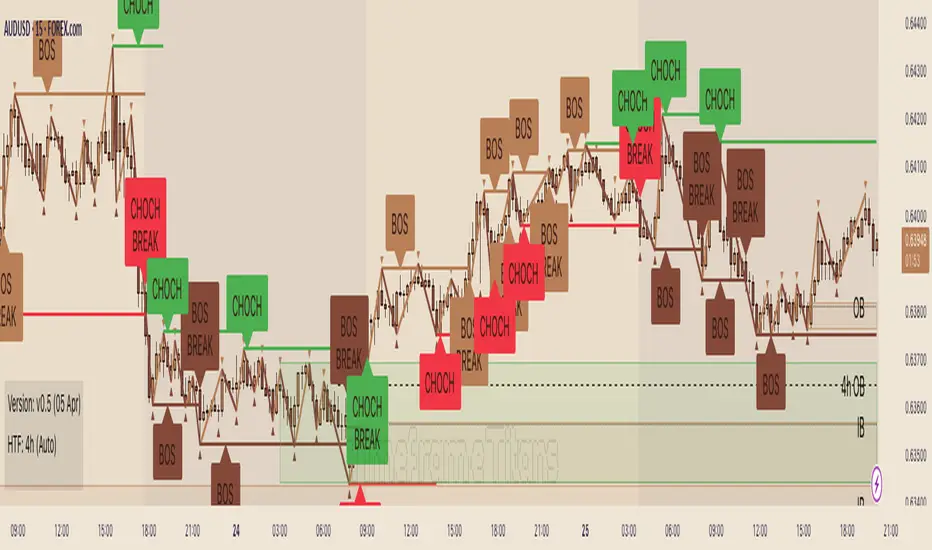
Here is a random example we found on the recent GBPUSD chart. In the screenshot below, the left chart is at 30m and the right is at 5m. We've toggled various settings to make the chart clearer for demonstration purposes.
1 — We get a CHoCH break on the higher timeframe. So our bias (if we are trying to trade with the trend) is bearish. Now we look for some other confluence.
2 — Price revisits the top of the range and mitigates an imbalance block. It wicks the CHoCH (resetting it) but does not break it on close. The bearish market structure is thus preserved. For these reasons, we're thinking about a short, and we switch to the 5m chart on the right to find an entry. We've chosen a Custom HTF of 30m to match the left chart and we can see the mitigated HTF order block, marked "30m IB". We can see when price moves definitively out of the order block area to the downside.
3 — A bearish order block is formed and very quickly price comes back into it. We could enter a short here with a stop above the closest relevant fractal.
4 — Another bearish order block forms and price retests it. Another entry. Two previous 5m bullish order blocks at the bottom of the chart act as support. We could potentially close our short here.
5 — Another test of the same block, which was not mitigated the first time. Another potential short entry. As it happens, price makes a massive run lower here, such that we could trail our stop down one ATR above every single high fractal (marked out using manual rays and a public ATR indicator) for a good R:R, but that's not the point.
This is a made-up, retrofitted example with a fairly generic methodology. It's just to show how some of the features of this indicator could be used in trading:
• Market structure can give a bias. It can also mark interesting levels.
• Using multiple timeframes, while more complex, can level up your trading experience.
• Price trading back into order blocks can be a good R:R entry.
Your actual way of trading, your playbook of setups, your knowledge of your strengths and weakness as a trader, is your own.
🟩 LIMITATIONS
This indicator is intended for use on Forex markets, although order blocks and market structure do form on any reasonably liquid asset.
The HTF uses confirmed data, so you need to wait until the HTF bar is closed before the order block can form. Therefore it does not repaint, in the sense that people worry about repainting, of changing data in the past. We use the latest recommended method of fetching HTF data .
The market structure uses live chart data, so structure and order blocks that are created by conditions on an open realtime bar can appear and disappear as the current bar close changes. This is quite normal .
The Williams pivots are by definition only confirmed after a defined number of bars, and like everyone else we plot them offset into the past.
Similarly, we offset order blocks into the past so that they start on the candle that has the high or low that defines the order block, not the candle that created them. For HTF order blocks, we calculate the number of chart bars back assuming a 24-hour market, which gives accurate offsets only on Forex and other symbols that trade close to 24 hours each day.
🟩 COMPARISON WITH OTHER INDICATORS
There are a great number of market structure and order block indicators already published on TradingView. Since there are only a certain number of highs and lows on the chart from which to produce structure and order blocks, they all look somewhat similar. However, this indicator, written entirely from scratch without reference to the code of any other indicators, is unique and original in two kinds of ways: in patterns and in features.
PRECISE PATTERNS
We believe that edge in trading can be found in, amongst other things, precision in analysis. You can't truly trust your backtests if your system is not repeatable, and your system is repeatable only if its definitions are precise.
We trade with this indicator, and our students trade with it as well. Why did we spend months creating a new indicator instead of using one of the many existing ones, most of which are free and open source?
Because they are not quite how we wanted.
The indicator was created from our proprietary structure rules, which are based on the generally accepted understanding of market structure, with some specific tweaks.
To prepare this description (after the indicator is finished), we searched for "Market Structure", "CHoCH", and "SMC" and list below all popular (with over 3K boosts; excluding invite-only) indicators that show market structure with CHoCH (sometimes called MSS). We configured the settings to most closely match how our indicator works, added both indicators to the same chart, and looked for relevant differences.
The purpose of this section is not to try to say that this indicator is better than any other, but just that it is different. This difference is important for us and our students.
Indicator #1
As you can see, the indicator interpreted the first part of the chart as a downtrend, whereas ours interpreted it as an uptrend. The structure is completely different, because our Williams Fractal lookback is 2, and the minimum "Swing Points" value for Indicator #1 is 10. Although this indicator is deservedly popular, it isn't what we can use for the way we trade.
Indicator #2
Setting the "Zigzag Length" to 2 results in wildly different market structure, as shown below. For many fractals, this indicator does not place the zigzag at the highest high or lowest low, as ours does consistently. It does not highlight the trend in any way. It gives many Market Structure Breaks in a short period. Although it's again wildly popular, it doesn't match our way of encoding market structure.
Indicator #3
Again, setting the "Pivot lb" and "Pivot rb" inputs to 2 gives much too sensitive market structure. This is because this indicator does not require, as we do, a counter-fractal to form after a fractal in order to confirm a BOS. We believe that this rule gives less noisy structure while also being responsive. Most indicators attempt to compensate for this by having a much larger lookback period. While this does of course give fewer pivots and less noise, this is simply a different logic and gives different results. Note also that although this indicator correctly defines the first section of the chart as an uptrend, it does not draw a CHoCH line. As discussed above, our definition of market structure means that there should always be one and only one active CHoCH line, and we draw this at the earliest sensible opportunity.
Indicator #4
Again, the lack of any extra pivot confirmation logic means that this indicator creates different structure with the same lookback period. Also note the lack of initial CHoCH.
Indicator #5
The lowest lookback is 3, and so this indicator too gives very different structure.
Indicator #6
Of course, using a lookback of 2 gives different structure with this indicator too. For variety, here we show a lookback of 5, which is the lowest setting that returns significantly less noisy structure. You can see that the main CHoCH at the top of the chart is similar but not at the same place. Increasing the lookback does not ever result in a CHoCH at the same place, because the logic is simply different. When the lookback increases above 10, no CHoCH lines are drawn at the top at all.
Indicator #7
This indicator uses the highest/lowest price for the last 10 bars (fixed), along with some other bar conditions. You can see the resulting structure is quite different. Among other differences, it does not create a BOS at the top of the chart, even in an uptrend, and it does not create an opposing CHoCH when the existing CHoCH is broken.
Indicator #8
With "Custom" market structure and a length of 2, BOS and CHoCH lines are drawn by this indicator but in incongruous places.
Conclusion
Although we only illustrate the top few alternatives, we did check many, many others.
These market structure indicators may produce useful output, but their structure differs significantly from ours. We didn't even need to get into specific examples because the general approaches are so different. It is up to the user to decide which indicator, and which interpretation of market structure, best suits their needs.
ORDER BLOCKS
Continuing, we illustrate differences with the most popular order block indicators, trying to get them to match our order blocks. Note that some of these are also in the previous list as market structure indicators.
Order blocks are always formed at swings when price moves away with force, so they will be sort of the same across all the very many existing order block indicators. We are looking for precision and differentiation, as we did with market structure.
Indicator #1
This indicator does not have ability to display mitigated order blocks, only active ones. The order blocks do not match at all.
Indicator #2
With a period of 2, this indicator marks many of the same order blocks as ours. It doesn't extend the blocks, and doesn't mark them when mitigated. The logic for choosing the order block candle is also clearly different.
Indicator #3
Even with very sensitive settings, this indicator did not create as many order blocks as ours and they are quite different.
Indicator #4
Again you can see the logic for choosing candles and creating blocks is simply different. This indicator has inadequate protection against empty arrays, which causes runtime errors on charts with not much history (not a problem for Forex charts in general, but noticeable on the testing chart).
Indicator #5
We were unable to get the order blocks to extend with this indicator, although it should be possible. Anyway the blocks are wildly different.
Indicator #6
Even with the most sensitive settings, this indicator showed only one order block on our test chart.
Indicator #7
This indicator incorporates complex price action concepts. Nevertheless, the order blocks are very different indeed.
Indicator #8
This indicator forms quite different blocks to ours. It has several interesting settings including a choice of using the candle body or wick.
Indicator #9
We were not able to configure this indicator to produce the same order blocks as ours.
Indicator #10
On very sensitive settings, this indicator matches many of our order blocks, but at the same time many are different.
Conclusion
None of the indicators tested here (nor the many others we looked at previously) use the same logic as ours. The differences are so obvious that we don't have to call out individual blocks and analyse how they differ.
Fundamentally, other indicators seem to use variable precision for pivots in their order block detection calculations. Our order blocks are pure candle patterns with two different rulesets for Standard Order Blocks and Imbalance Order Blocks, and this logic does not change.
Note that our order blocks do not always automatically extend to the swing high or low, nor allow the user to choose the limit of the block, but use unique rules.
In summary, our indicator differs from other order block indicators in terms of fundamental detection logic, candle placement, boundary definition, mitigation levels, and logical states (see below).
UNIQUE COMBINATION OF FEATURES
In comparison to all other indicators we looked at, our indicator:
• Uses order blocks with three states: active, mitigated, and partially mitigated. Our mitigation lines for order blocks are rules-based. If price touches the mitigation line, the order block is considered fully mitigated. If price goes inside the order block but does not hit the mitigation line, it is only partially mitigated. These three states are visually distinguished.
• Has the most extensive visual customisation options of all those we looked at. We believe that being able to customise how you see indicator outputs is very important for reducing mental load while analysing and trading.
• Has a unique feature that combines market structure and order blocks, where the user can choose to show pro-trend order blocks (bullish blocks that are formed in bullish structure and vice-versa) or counter-trend blocks (bullish blocks that are formed in bearish structure and vice-versa).
• Approximates an initial trend bias very quickly, so we can start creatng BOS, CHoCH, etc.
• Requires a counter pivot to confirm a BOS line. This seemingly small logical step actually creates very different structure, as we saw in the comparison section.
• Uses a sophisticated array-based sorting mechanism to preserve the selected number of imbalances, use the rest of the TradingView box allowance for order blocks, and delete excess order block objects (not just drawings) in reverse historical order.
• Hides order block drawings if they are a configurable distance away from price. Magically redraws them if price moves closer.
• Includes an equivalent to the system "Calculated bars" setting for the high timeframe, to avoid unnecessary processing and improve performance.
🟩 CODING CONSIDERATIONS
This indicator consists of all original code written by @SimpleCryptoLife for Timeframe_Titans.
AI was used for the following purposes:
• Autocomplete
• Checking that bullish and bearish logic is parallel in a given function
• Querying the names and locations of variables hundreds of lines away when we forgot what they're called, like an expensive search-and-replace
• Help with debugging (it usually makes up elaborate and wrong ideas though)
It was not used to replace the coder's expertise and creativity, or to "vibe-code" some black-box functionality we didn't understand. We can recommend that you use AI the same way.
═════════════════════════════════════════════════════════════
SwiftEdge NW EnvelopeSwiftEdge NW Envelope
Overview
The SwiftEdge NW Envelope is a visually striking technical indicator designed for traders seeking to identify high-probability buy and sell opportunities in volatile markets. By combining the Relative Strength Index (RSI), Average True Range (ATR), and Nadaraya-Watson Envelope, this indicator provides a unique blend of momentum, volatility, and non-linear trend analysis. Its futuristic, AI-inspired aesthetic—featuring neon gradients and dynamic colors—enhances chart readability while delivering actionable trading signals.
What It Does
The SwiftEdge NW Envelope generates buy and sell signals based on price interactions with dynamically calculated support and resistance bands, confirmed by RSI conditions. The indicator:
Plots a Nadaraya-Watson Envelope to identify smooth, non-linear price trends and dynamic support/resistance zones.
Uses ATR to scale the envelope’s bands, adapting to market volatility.
Employs RSI to confirm overbought/oversold conditions, ensuring signals align with momentum.
Visualizes signals with neon-colored markers, background zones, and labels for intuitive decision-making.
How It Works
The indicator integrates three key components:
Nadaraya-Watson Envelope:
A kernel-based regression technique that smooths price data to create a central trend line (mean) and dynamic upper/lower bands.
Unlike traditional moving averages, it provides a non-linear, adaptive view of price trends, making it ideal for capturing complex market movements.
The band width is determined by ATR, ensuring responsiveness to volatility.
Average True Range (ATR):
Measures market volatility to scale the envelope’s bands.
A multiplier (default: 0.5) adjusts the sensitivity of the bands, allowing traders to fine-tune the indicator for different assets or market conditions.
Relative Strength Index (RSI):
A momentum oscillator with a shortened period (default: 5) for increased sensitivity.
Confirms buy signals when RSI is oversold (default: <30) and sell signals when RSI is overbought (default: >70).
Signal Logic
Buy Signal: Triggered when the price crosses above the lower band of the Nadaraya-Watson Envelope and RSI is below the oversold threshold. Marked by a green circle and a "BUY" label below the candle.
Sell Signal: Triggered when the price crosses below the upper band and RSI is above the overbought threshold. Marked by a magenta circle and a "SELL" label above the candle.
Background Zones: Green (buy) or red (sell) translucent zones highlight signal areas for quick recognition.
Visual Features
Dynamic Colors: The central trend line shifts between cyan (uptrend), purple (downtrend), or gray (neutral) based on price position relative to the mean.
Neon Gradient Fill: A translucent blue fill between the upper (green) and lower (red) bands creates a glowing, futuristic effect.
Modern Signal Markers: Small, vibrant circles (green for buy, magenta for sell) and clear labels enhance visual clarity.
Why This Combination?
The SwiftEdge NW Envelope combines RSI, ATR, and Nadaraya-Watson Envelope to create a robust trading tool:
RSI provides momentum confirmation, filtering out false signals in choppy markets.
ATR ensures the envelope adapts to changing volatility, making it suitable for both trending and ranging markets.
Nadaraya-Watson Envelope offers a sophisticated, non-linear alternative to traditional bands (e.g., Bollinger Bands), capturing subtle price dynamics. Together, these components deliver a balanced approach to trend-following and mean-reversion strategies, with RSI acting as a gatekeeper to improve signal reliability.
Customize Settings:
RSI Period (5): Adjust for more/less sensitivity to momentum.
RSI Overbought/Oversold (70/30): Modify thresholds to tighten or loosen signal conditions.
ATR Period (14) and Multiplier (0.5): Tune volatility sensitivity.
NW Length (25), Bandwidth (8.0), Multiplier (3.0): Adjust the smoothness and width of the envelope.
Interpret Signals:
Buy: Look for green circles and "BUY" labels when price crosses above the lower band, confirmed by low RSI.
Sell: Look for magenta circles and "SELL" labels when price crosses below the upper band, confirmed by high RSI.
Use background zones to quickly spot active signal areas.
Combine with Other Tools:
Pair with support/resistance levels or volume analysis for additional confirmation.
Test signals on a demo account before live trading.
Originality
The SwiftEdge NW Envelope stands out due to:
Its innovative use of Nadaraya-Watson regression, a less common but powerful tool for non-linear trend analysis.
A unique visual design with neon gradients and dynamic colors, inspired by AI and futuristic interfaces, making it both functional and visually engaging.
A streamlined signal system that balances momentum (RSI), volatility (ATR), and trend (Nadaraya-Watson), reducing noise and enhancing trade precision.
Notes
Best suited for volatile markets (e.g., forex, crypto, stocks) where price swings create clear envelope breakouts.
Adjust input parameters to match your trading style (e.g., shorter RSI period for scalping, wider bands for swing trading).
Always backtest and validate signals in your specific market and timeframe before trading.

Altcoins Screener [SwissAlgo]Introduction: The Altcoins Screener at a Glance
The Altcoins Screener is a cryptocurrency analysis tool designed to provide an overview of potential trading opportunities across multiple crypto coins/tokens and categories. By combining technical analysis, price action assessment, and social metrics (via LunarCrush data), it presents market information and trading signals for a broad range of altcoins (approx. 300 USDT.P pairs of 9 crypto categories).
The screener is designed to consolidate market information onto a single chart , aiming to streamline the analysis of market conditions. It provides a consolidated market overview, which can simplify the assessment of market conditions, compared to monitoring individual charts with several layered indicators.
Key Features:
🔹 Multi-category analysis covering 300 crypto pairs of 9 categories on a single chart (Layer 1 & Top Coins, Layer2 & Scaling, Defi & Landing, Gaming & Metaverse, AI & Data, Exchanges & Trading, NFT & Social, Memes & Community, Other, User's Custom Portfolio).
🔹 Technical analysis with trade signals (Long/Short) based on an aggregated view of technical and social data points
🔹 Social sentiment integration through LunarCrush metrics (GalaxyScore, AltRank, Social Sentiment)
🔹 Real-time market scanning provides automated alerts when market conditions for specified coins/tokens potentially change.
🔹 Custom watchlist support for personalized monitoring (users can define a custom category containing a set of specific cryptocurrencies, i.e. own portfolio).
The screener presents data in a table format, using color-coded indicators to aid visual analysis. Detailed technical information is also provided. The assessments/trade signals provided by this indicator should be considered as one input among many when forming your trading strategy.
--------------------------------------
What It Does
The Altcoins Screener is a cryptocurrency analysis tool that offers:
Data Display and Analysis (Technical/Social):
🔹 Technical Metrics
* Technical Raw Data : Displays raw values for a range of technical indicators, including RSI, Stochastic RSI, DMI/ADX, RVI, ATR, OBV, and Hull Moving Averages (including their recent trends and potential significance).
Detailed view of key technical indicators, for further analysis and evaluation:
* Technical Analysis (Summary) : Provides a summarized interpretation of technical conditions based on aggregated parameters:
* Price Action
* Trend
* Momentum
* Volatility
* Volume
Summarized view of confluences for potential long/short bias:
🔹 Social Metrics (LunarCrush) : Presents data from LunarCrush®, including Galaxy Score®, AltRank®, and Social Sentiment® (including their recent trends and potential significance).
Lunarcrush data for the top 10 coins for each crypto category:
🔹 PVSRA (Price Volume & Market Makers Activity) Candles : Shows special candles highlighting potential market maker activity and volume anomalies, helping identify possible manipulation zones (including imbalance zones, i.e. price areas that market makers may revisit)
--------------------------------------
Key Features:
Automated trade signals (Long/Short) are generated based on algorithmic calculations and signal confidence levels across technical and social data points. These signals are intended to be used as one component of a broader trading strategy.
Custom sensitivity settings allow users to adjust the analysis timeframe (options: 1D, 2D, or 1W). Higher timeframes may provide a broader perspective, while the 2D setting is the default configuration.
Multi-category analysis covering a selection of approximately 300 crypto pairs across 9 predefined crypto categories.
Custom symbol selection: Users can define a custom list of up to 10 symbols for focused monitoring.
Automated Alerts to track potential trend changes across crypto categories (Long to Short to Neutral, or vice versa)
Visual Interface:
Organized table display with color-coded indicators to aid interpretation.
Clear and efficient format for scanning market information.
--------------------------------------
Target Audience
🔹 The screener is designed for cryptocurrency traders who:
Need to efficiently monitor multiple USDT perpetual futures markets
Use technical analysis in their trading decisions
Want to track sector-wide movements across crypto categories
🔹 Suitable for different trading styles:
Scalpers requiring quick market assessment
Swing traders analyzing multi-day trends
Position traders monitoring longer-term setups
The color-coded interface makes it accessible for intermediate traders while providing detailed metrics for advanced users. A basic understanding of technical analysis and crypto trading is recommended.
--------------------------------------
How It Works
The Altcoins Screener evaluates cryptocurrencies through a multi-layered analysis:
🔹 Core Analysis Components
Each parameter combines multiple indicators for comprehensive evaluation:
Price Action
EMA crossovers and momentum
Support/resistance zones
Candlestick patterns
Trend
Hull Moving Average system
DMI/ADX trend strength
Multi-timeframe confirmation
Momentum
RSI/Stochastic RSI readings
MACD convergence/divergence
Oscillator confirmations
Volatility
RVI/ATR measurements
Bollinger Bands behavior
Historical volatility trends
Volume
OBV trend analysis
Volume/price correlations
Volume profile assessment
🔹 Signal Generation Process
1. Real-time data collection across timeframes
2. Weighted indicator calculations
3. Parameter aggregation and analysis
4. Signal strength determination
5. Color-coding and alert generation
--------------------------------------
How to Use
🔹 Initial Setup:
Add the indicator to a chart (use the 1D timeframe)
Select your preferred crypto category or create a custom list
Choose between Technical Analysis or Technical Metrics view
Set data sensitivity based on your trading style
🔹 Using the Technical Analysis View:
Monitor color-coded dots for quick market assessment
Green: bullish conditions
Red: bearish conditions
Gray: neutral conditions
Check the "Trade Signal" column for potential Long/Short entries signaled by confluences among technical and/or social data points
🔹 Using the Technical Metrics View:
Review detailed numerical values
Monitor slopes (↑↓ arrows) for the most recent trend direction of each data point
Watch for pivotal points (highlighted cells): these are data points that suggest potential trend reversals
Focus on the confluence of multiple indicators
The technical metrics view corroborates the conclusions shown in the Technical Analysis View, providing more details about some critical data points.
🔹 Alert Configuration:
Enable Technical Alerts for signal notifications (which coin/token seems most suited for Long or Short trades, and which coin/token is in a neutral/uncertain state for trading = "No Trade")
Configure alert conditions based on trading style
Set timeframe-appropriate sensitivity
Monitor alert messages for trade signals
Instructions on how to set alerts are provided in the script (enable "Signals Setup Instructions" in User Interface to get a step-by-step guide about setting up alerts)
Best Practices:
Confirm signals across multiple timeframes
Use appropriate sensitivity for your trading style
Monitor multiple categories for sector rotation
Combine signals with your trading strategy
Verify signals with price action confirmation and deep dive into the charts of your potential targets
--------------------------------------
About the Settings
🔹 Crypto Category Selection
Layer 1 & Major: Top market cap coins (BTC, ETH, XRP,...), established protocols
Layer 2 & Scaling: ETH L2s, scaling solutions
DeFi & Lending: Decentralized finance protocols
Gaming & Metaverse: Gaming and virtual world tokens
AI & Data: Artificial intelligence and data projects
Exchange & Trading: Exchange tokens, trading protocols
NFT & Social: NFT platforms, social tokens
Memes & Community: Community-driven tokens
Others & Misc: Other categories
Custom Category: User-defined list (up to 10 symbols)
Data Type Options
Technical Analysis: Color-coded summary view
Technical Metrics: Detailed numerical values of some key technical data points
Sensitivity Settings
Higher: Shorter timeframe, more frequent signals
Default: Balanced timeframe, standard signals
Lower: Longer timeframe, stronger signals
Alert Settings
Technical Alerts: Trade signal notifications
Data Timeframe: Minimum 1D required
Theme: Dark/Light mode options
Note: All analysis is performed on USDT Perpetual Futures pairs from Binance
--------------------------------------
FAQ
Q: Does the screener work on other exchanges besides Binance?
A: No, it's designed specifically for Binance USDT Perpetual Futures pairs. Binance offers the highest liquidity and trading volume in the crypto derivatives market, making it ideal for technical analysis. The extensive range of trading pairs and reliable data streams help ensure more accurate signals and analysis. Using a single high-liquidity exchange also helps avoid inconsistencies that could arise from aggregating data across multiple platforms with varying liquidity levels.
Q: What's the minimum timeframe required?
A: The screener requires a minimum 1D (daily) timeframe. This requirement ensures that the technical analysis has sufficient data points for reliable signal generation. Lower timeframes can produce more noise and false signals, while daily timeframes help filter out market noise and identify stronger trends.
Q: Why are some social metrics showing "NaN"?
A: "NaN" (Not a Number) appears when cryptocurrencies don't have associated LunarCrush data. This typically occurs with newer tokens or those with lower market caps. The technical analysis remains fully functional regardless of social metric availability, as these are complementary data points.
Q: How often are signals updated?
A: Signals update with each new candle on the selected timeframe (1D, 2D, or 1W). For example, on the default 2D setting, signals are recalculated every two days as new candles form. This helps reduce noise while maintaining timely analysis of market conditions.
Q: Can I add spot trading pairs?
A: No, the screener is optimized for Binance USDT perpetual futures pairs for data consistency and analysis purposes. While spot and perpetual prices typically align closely due to arbitrage, using a single data source (Binance) and contract type (USDT perpetual) ensures uniform data quality and analysis across all pairs. This standardization helps maintain reliable technical analysis and signal generation.
Q: How many coins can I add to my custom list?
A: Users can add up to 10 custom symbols to their watchlist. This limit is designed to maintain optimal performance while allowing focused monitoring of specific assets. The custom list complements the predefined categories that cover over 300 pairs.
Q: What determines signal confidence levels?
A: Signal confidence is calculated through a weighted algorithm that considers multiple factors: trend strength (Hull MA, DMI/ADX), momentum indicators (RSI, SRSI), volatility measurements (RVI, ATR, BB), volume analysis (OBV, volume trends), and price action patterns. Higher confidence levels indicate stronger alignment across these factors.
Q: Are signals guaranteed to work?
A: No. Signals are analytical tools based on historical and current market data, not guaranteed predictions. They should be used as one component of a comprehensive trading strategy that includes proper risk management, position sizing, and additional confirmation factors. Past performance does not guarantee future results.
Q: Why does the screener need higher timeframes?
A: Higher timeframes (1D minimum) provide several benefits: reduced market noise, more reliable technical signals, better trend identification, and lower likelihood of false signals. They also align better with institutional trading patterns and allow for a more thorough analysis of market conditions across multiple indicators.
--------------------------------------
Conclusion
The Altcoins Screener is a comprehensive crypto market analysis tool that:
Scans 300+ cryptocurrencies across 9 sectors on a single chart
Combines technical indicators and social metrics for signal generation
Identifies potential trading opportunities through color-coded visuals
Saves time by eliminating the need to monitor multiple charts
The tool is suited for:
Market overview and sector rotation analysis
Quick assessment of market conditions
Technical and social sentiment tracking
Systematic trading approach with alerts
Use this screener with caution and as a complement to any other tool you use to define your trading strategy.
--------------------------------------
Disclaimer
This indicator is for informational and educational purposes only:
Not financial advice: This indicator should not be considered investment advice.
No guarantee of accuracy: The indicator's calculations and signals are based on specific algorithms and data sources, but accuracy cannot be guaranteed. Market conditions can change rapidly.
Past performance is not predictive: Past performance of the indicator's signals or any specific asset is not indicative of future results.
Substantial risk of loss: Trading cryptocurrencies involves a substantial risk of loss. You can lose money trading these assets.
User responsibility: Users are solely responsible for their own trading decisions and should exercise caution.
Independent research required: Always conduct thorough independent research (DYOR) before making any trading decisions.
Technical analysis is one of many tools: Technical analysis, including the output of this indicator, is just one tool among many and should not be relied upon exclusively.
Risk management is essential: Use proper risk management techniques, including position sizing and stop-loss orders.
Comprehensive strategy: Use this tool as part of a comprehensive trading strategy, not as a standalone solution.
No liability for trading results: The Author assumes no responsibility or liability for any trading results or losses incurred as a result of using this indicator.
No TradingView affiliation: SwissAlgo is an independent entity and is not affiliated with or endorsed by TradingView.
LunarCrush data: The indicator utilizes publicly available data from LunarCrush. LunarCrush data and trademarks are the property of LunarCrush.
Consult a financial advisor: Consult with a qualified financial advisor before making any investment decisions.
By using this indicator, you acknowledge and agree to these terms. If you do not agree with these terms, please refrain from using this indicator.

RSI MACD Combined Color StrategyOverview
This indicator combines RSI and MACD signals to create a powerful visual trading system, inspired by TrendSpider's AI Strategy Coder examples. It colors candles based on the alignment of three key technical conditions, providing clear visual signals for potential trend strength and direction.
Technical Components
Core Conditions
RSI (Relative Strength Index) > 50
Indicates bullish momentum when price is trading above the centerline
Traditional indicator of trend strength
MACD Line > Signal Line
Shows positive momentum
Classic signal for potential upward movement
MACD Line > 0
Confirms bullish territory
Indicates overall positive momentum
Color Coding System
🟢 Green Candles: All three conditions are met
Strongest bullish signal
Suggests high probability trading opportunities
⚪ Grey Candles: One or two conditions are met
Neutral or transitioning market
Suggests caution or waiting for stronger confirmation
🔴 Red Candles: No conditions are met
Bearish signal
Suggests potential downward pressure
How to Use This Indicator
For Entry Signals
Look for transitions from red or grey to green candles
Green candles suggest strong bullish alignment
Consider entering long positions when candles turn green
For Exit Signals
Watch for color transitions from green to grey or red
Consider taking profits when candles change from green to grey
Consider stop losses when candles turn red
Risk Management
Use color transitions as part of your broader strategy
Don't rely solely on color changes for trading decisions
Combine with other technical analysis tools and risk management practices
Customizable Parameters
RSI Length (default: 14)
MACD Fast Length (default: 12)
MACD Slow Length (default: 26)
MACD Signal Length (default: 9)
Best Practices
Use multiple timeframes for confirmation
Look for confluences with support/resistance levels
Consider volume and market context
Start with default settings and adjust based on your trading style
Backtest different parameter combinations
Notes
This indicator works best in trending markets
Grey candles can indicate transition periods
Consider market conditions and volatility when interpreting signals
Credits
Inspired by TrendSpider's AI Strategy Coder examples and adapted for TradingView using Pine Script v5.
Disclaimer
This technical indicator is for informational purposes only. Always conduct your own analysis and consider risk management principles before making trading decisions. Past performance does not guarantee future results.

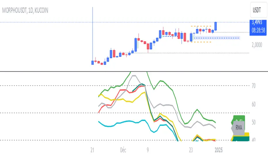
RSI NarrativesDescription:
The RSI Narratives script aggregates Relative Strength Index (RSI) values across multiple cryptocurrency narratives or sectors, providing an easy-to-read visual and alert system for trend reversals and overbought/oversold conditions. This tool is designed for traders looking to track sector-specific trends and compare performance across AI, DeFi, Level 1 blockchains, and more.
Key Features:
RSI Aggregation by Sector: Calculates average RSI for key narratives, including AI, DeFi, Level 1 blockchains, new memes, and more.
Customizable RSI Settings: Adjust RSI period, line width, and label offsets for personalized analysis.
Dynamic Alerts: Receive alerts when a narrative enters overbought or oversold territory, helping you act quickly on market movements.
Clean Visualization: Overlay sector-specific SMA lines with distinct colors and optional labels for quick interpretation.
Multi-Narrative Comparison: Analyze trends across diverse narratives to identify emerging opportunities.
Parameters for Customization:
RSI Period: Set the lookback period for RSI calculations (default: 14).
Line Width: Adjust the thickness of plotted lines (default: 2).
Label Offset: Control label placement for better chart readability.
Overbought/Oversold Thresholds: Configure the RSI levels for alerts (default: 70/40).
How to Use:
Add the script to your TradingView chart.
Customize the RSI parameters to suit your trading strategy.
Monitor the plotted SMA lines to identify narrative-specific trends.
Set alerts for overbought and oversold conditions to stay informed in real time.
Alerts System:
Alerts trigger when a narrative crosses predefined overbought or oversold levels.
Text notifications suggest potential trading actions, such as selling on overbought or buying on oversold.
Intended Users:
This script is ideal for crypto traders, sector analysts, and market enthusiasts who want to track performance across narratives and gain actionable insights into sector rotations.
Disclaimer:
This script is for educational and informational purposes only. It does not constitute financial advice. Please test on historical data and practice caution when trading.
Crypto Sectors Performance [Daveatt]IMPORTANT
⚠️ This script must be used on the Daily timeframe only.
OVERVIEW
This indicator brings the powerful sector analysis capabilities from velo.xyz/market's
Sector Performance chart to TradingView.
It enables traders to track and compare performance across the crypto market's major sectors, providing essential insights for sector rotation strategies and market analysis.
CALCULATION METHOD
The indicator calculates performance across six key crypto sectors: DeFi, Gaming, Layer 1s, Layer 2s, AI, and Memecoins.
For each sector, it computes a rolling percentage performance by averaging the performance of multiple representative tokens.
All sector performances are rebased to 0% at the start of each period, making relative comparisons clear and intuitive.
VISUALIZATION MODES
The script features two distinct visualization methods:
Plots Mode:
Displays continuous performance lines for each sector over time, ideal for tracking relative strength trends and sector momentum. Each sector has its own color-coded line with performance values clearly marked.
Bars Mode:
Presents current sector performance as vertical bars, offering an immediate visual comparison of sector gains and losses.
The bars are color-coded and labeled with exact percentage values for precise analysis.
For the "Bars Mode", I used the box.new() function
SECTOR COMPOSITION
Each sector comprises carefully selected representative tokens:
- DeFi: AAVE, 1INCH, JUP, MKR, UNI
- Gaming: GALA, AXS, RONIN, SAND
- Layer 1: BTC, ETH, AVAX, APT, SOL, BNB, SUI
- Layer 2: ARB, OP, ZK, POL, STRK, MNT
- AI: FET, NEAR, RENDER, TAO
- Memecoins: PEPE, BONK, SHIB, DOGE, WIFU, POPCAT
PERFORMANCE TRACKING
The indicator implements a rolling window approach for performance calculations.
Starting from 0% at the beginning of each period, it tracks relative performance with positive values indicating outperformance and negative values showing underperformance.
Multiple timeframe options (1W, 1M, 3M, 6M, and 1Y) allow for both short-term and long-term analysis.
APPLICATIONS
This tool proves invaluable for:
- Sector rotation analysis
- Identifying trending sectors
- Comparing relative strength
- Gauging market sentiment
- Understanding market structure through sector performance
Thanks for reading and for the support
Daveatt

The Ultimate Indicator by ATK
The Ultimate Indicator By ATK
This all-in-one trading indicator integrates multiple advanced tools to provide ICT traders with deep insights into market structure, liquidity zones, Fair Value Gaps (FVG), and AI-powered signals. Whether you’re a scalper or a long-term trader, this indicator offers real-time analysis and helps identify potential trading opportunities in dynamic markets.
🔵 Key Features
🔹 2 options for checking SMT (Separation and Divergence) Detection:
First - Compares highs and lows of a primary symbol (e.g., NQ1!) with a user-defined comparison symbol (e.g., ES1!).
Automatically detects and visualizes discrepancies (red for highs, blue for lows) between the symbols.
Offers customizable comparison settings and alerts for divergence detection.
Second -
Real-time SMT comparison between two tickers - red/green lines.
🔹 Market Structure Change (MSS) & Break of Structure (BOS) Detection:
Identifies market structure shifts and breakouts, crucial for spotting potential reversals.
Customizable sensitivity and length settings to adapt to various market conditions and trading strategies. Use 3 different timeframes on the same chart.
🔹 Buy Side & Sell Side Liquidity Zones:
Highlights liquidity zones on both buy and sell sides, offering a clear view of market pressure points.
Configurable settings for detection length, margin, and alert conditions for liquidity sweeps like the 15-minute Buy Side Liquidity (BSL) and Sell Side Liquidity (SSL).
These lines from Swing Highs & Lows:
Automatically plots horizontal lines at the most recent swing highs and lows.
Lines are removed once the closing price breaches these levels, ensuring real-time updates and clean charting.
🔹 Fair Value Gap (FVG) Detection:
Detects FVG formations on 5-minute and 1-minute charts, making it ideal for scalpers capturing liquidity gaps.
Includes directional arrows and customizable alerts based on higher and lower timeframe FVG analysis, helping traders time their entry and exit points.
🔹IFVG (Inverse fair value gap) - yellow
🔹IFVG + SMT - Light blue
🔹IFVG + SMT + HTF FVG - green/red (1 min only)
🔹IFVG + SMT + BSL/SSL Swept - green/red (1 min only)
for example:
🔹 Capture and plot significant price levels at specific times throughout the trading day:
TDO (True Day Open): The price at which a market opens at 12:00 AM US.
TMSO (True Micro Session Open): The open price of the Q2 of the micro session.
RVT (Revolving True Open): The price recorded at 12:00 PM US.
AO (Asia True Open Price): The price captured at 7:30 PM US, specifically representing the opening price of the Asian session.
LO (London True Open Price): 1:30 AM US
AM (New York Session - Afternoon Market True Open Price): 7:30 AM US
PM (Post Market Open Price): 1:30 PM US.
For example TMSO:
🔹 AI-Powered Entry Detection:
The script helps identify entry points based on specific candle patterns, while also considering the exponential moving averages (EMAs) for trend confirmation.
🔶FFMS Strategy: (First Five Minute Strategy)
Check 5-min time frame if the price is between the high and low of the previous day. then, when NYO if there is retest on the High/Low on the 5-min chart after crossover or crossunder the 5 minute first candle high/low lines.
🔶PSP & PSP + FVG
🔹The Precision Swing Point (PSP). It helps you visually identify price decorrelation (type of SMT) among key futures contracts (NQ/ES or NQ/ES/YM/ZB) and set alerts for these significant market movements.
🔹The PSP HTF 15 Min + FVG LTF 1 Min
In this strategy the script is looking for PSP in HTF (15-Min) and capture the FVG in LTF (1-Min) only if its between High and Low of the PSP.
If there is a retracement in parallel micro session time, for example: Q1 with Q3 or Q2 with Q4, Q3 with Q1, etc…
if the retracement was happened and the price close above/below the high/low of the FVG from the LTF that captured according to the direction for long/short, it plots an arrow.
Update the script that checks the purple arrows and shows all of them each time there is a new PSP in a 15-minute timeframe and then FVG in 1 Min timeframe with the reference to the TDO/TMSO/Open session
for example:
Step 1: PSP 15Min LOW/HIGH Lines look for FVG by the conditions above - purple arrow
Step 2:FVG founded - purple arrow
SMT Fill on 15 min timeframe + IFVG 1 min - Detected option:
When Sym1 closed above/below FVG and Sym2 didn't it is SMT FILL (15 Min timeframe)
White arrows when captured SMT FIll + IFVG:
option to turn on alert on this strategy too.
🔹Detect liquidity swept on 15-min timeframe by $$ - green/red
🔹Detect liquidity to sweep zones on by diamonds - green/red
🔹Alerts for all Events and full scenarios.
Real-time notifications ensure traders can act quickly on potential trade setups.
🔵 Conclusion:
This Ultimate Indicator by ATK brings together critical elements of market analysis in one tool for ICT traders, offering real-time insights, alerts, and visual aids to enhance trading strategies. Whether you’re focused on short-term price action or long-term market trends, this indicator provides the tools necessary for informed decision-making and improved trading performance.
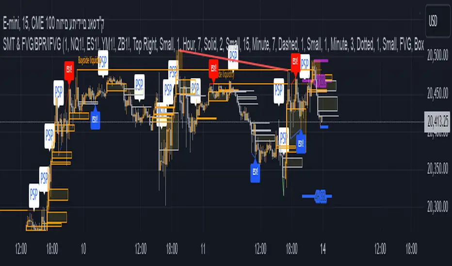
Sector Daily Gain/Loss TableOverview: The "Sector Daily Gain/Loss Table" is a custom TradingView indicator designed to display the daily percentage changes in selected cryptocurrency sectors. This indicator provides a comprehensive view of the performance of various cryptocurrencies organized into specific sectors, helping traders and analysts to make informed decisions based on sector performance.
Key Features:
Dynamic Data Retrieval: The indicator retrieves daily closing prices for multiple cryptocurrencies across different exchanges (Binance and Bybit) using the request.security function. This allows users to monitor real-time price movements.
Sectors Covered:
BTC Sector: Includes Bitcoin (BTC).
ETH Sector: Includes Ethereum (ETH).
RWA Sector: Comprises various assets such as OM, ONDO, POLYX, SNX, PENDLE, and HIFI.
L1/L2 Sector: Features major Layer 1 and Layer 2 solutions including ETH, BNB, SOL, XRP, TON, ADA, AVAX, DOT, SUI, APT, ICP, POL, and more.
MEME Sector: Showcases popular meme coins like DOGE, SHIB, PEPE, WIF, BONK, FLOKI, ORDI, BOME, and NEIRO, along with MEW and POPCAT from Bybit.
AI Sector: Highlights AI-related tokens such as TAO, FET, GRT, THETA, WLD, and TURBO.
DEFI Sector: Displays decentralized finance projects including UNI, AAVE, INJ, RUNE, MKR, JUP, LDO, PENDLE, CAKE, LUNA, RAY, OSMO, KAVA, and RSR.
Average Gain/Loss Calculations: For each sector, the indicator calculates the average percentage change in price based on the included cryptocurrencies, offering insights into sector-wide performance trends.
Table Display: The performance metrics are presented in a clean and organized table format on the TradingView chart, providing easy access to vital information for traders.
User-Friendly Design: The table is designed to be visually appealing and informative, with color coding and clear labeling for each sector and its corresponding percentage change.
Usage: Traders can utilize this indicator to quickly assess the performance of various cryptocurrency sectors and make informed trading decisions based on the daily changes in sector performance.
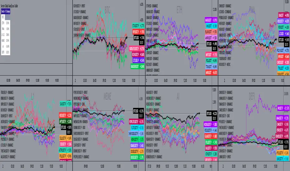
Altcoin ManagerThe Altcoin Manager is a comprehensive script for identifying the current altcoin narrative by tracking and analyzing of a wide array of altcoins across various blockchain layers and categories, such as DeFi, GameFi, AI, and Meme coins. Ideal for traders looking to get a broad yet detailed view of the altcoin market, covering various sectors and chains.
The Key Features:
Versatile Asset Tracking:
Tracks 40 different cryptocurrencies (as of publishing) across different categories, allowing for a diversified and detailed analysis of the altcoin market.
Customizable Assets and Category Analysis:
Select 20 of your own coins across 4 different categories such as DeFi, GameFi, AI, and Meme coins as well as specifying their individual chains.
Dynamic Layer and Chain Analysis:
Includes options to plot and analyze specific blockchain layers and chains such as Ethereum Chain, Solana Chain, BNB Smart Chain, Arbitrum Chain, and Polygon Chain. The script associates various assets with specific blockchains, providing a clearer picture of how different segments of the altcoin market are performing.
Cumulative and Per-Candle Change:
Switch between viewing the total cumulative change since a set start date or the per-candle change, offering flexibility in analyzing price movements over different timeframes.
Denomination Adjustment:
Includes a functionality to denominate asset prices in other currencies or crypto such as BTC, allowing for a more tailored financial analysis according to your preference.
Moving Averages for Categories and Chains:
Calculates and plots moving averages for each category and chain, aiding in the identification of trends over the selected moving average length.
How do I use it?
This script is not used with any particular chart. Instead, assign it it's own tab and layout.
For a clearer analysis, use multiple different panels to track Categories and Chains separately, both Cumulative for a longer term analysis and Per-Candle to find ongoing breakouts and changes in trend.
You can either use the pre-selected altcoins to represent the market, or you can select your own.
The Layer 1 and Layer 2 are not customizable but consists of 15 popular Layer 1 incl Bitcoin, Ethereum, Solana etc. Layer 2 consists of 5 popular Layer 2.

Trendmaster - Crypto Flow IndexWhat it is:
The Trendmaster Crypto Flow Index is a unique tool designed to give you an overview of the performance of different Crypto market sectors and sub-sectors. It helps you to identify where you should be focusing your investments for maximum portfolio efficiency and profitability.
What it does:
The Crypto Flow Index presents a visual overview of the flows of retail and institutional capital into the four main market sectors: Large Caps, Alts Coins, Shit Coins, and Stable Coins as well as several other sub-sectors. Each sector is assigned a "Flow Score", which indicates its current performance, demand, and strength in percentage terms. The "Flow Score" also provides insights into the current stage of the market cycle and the typical over and underperformances of assets that correlate to it. Additionally, the index factors in the sector have a "Correlation" to the broader market, allowing you to see the best sectors for trading and investing, either for positional hedging or differential plays.
How to Use it:
To use the Trendmaster Crypto Flow Index, you can simply observe the evolving colored line within the indicator and the table overview. You can identify which sectors are outperforming or underperforming the general market and make informed decisions about where to direct your focus and funds. By monitoring the transitions of Flow between sectors, you can gain invaluable insights into the market cycle and the typical over and underperformances of assets that correlate to it. This information will help you to maximize portfolio efficiency by targeting different market sectors based on their performance to the overall cryptocurrency market. The index covers different sectors, including Large caps, Alts, Shit, Stables, AI, Defi, Dex, Exchange, Gaming, Meme, Metaverse, Nft, Privacy, Smart, and Sports.
Examples of Cryptocurrencies represented in the different market sectors:
Large caps: The biggest market cap cryptocurrencies such as BTC and ETH.
Alts: High-cap and high-volume digital assets that are smaller than large caps, such as LTC and XRP.
Shit coins: Smaller cap projects that are highly speculative and experience significant price volatility, such as BAT and HOT.
Stables: Fiat-pegged assets that provide a stable value, such as USDT and USDC.
AI: Projects that are based on artificial intelligence, such as FET and AGIX.
DeFi: Leverages high volume smart contract platforms to provide financial products in crypto, mainly ERC20 tokens such as LINK and AAVE.
DEX: Decentralized exchanges with their own utility tokens, such as UNI and SUSHI.
Exchange: Centralized exchanges with their own utility tokens, such as BNB and CRO.
Gaming: Web3/crypto gaming platforms with their own utility tokens, such as AXS and GMT.
Meme: Similar to shit coins, but with no real functionality and based purely on social media and memes, such as DOGE and SHIB.
Metaverse: Projects that aim to provide Metaverse assets such as virtual land and assets, such as MANA and SAND.
NFT: Non-fungible tokens with their own token or NFT-based platforms that have their own utility tokens, such as APE and LOOKS.
Privacy: Anonymous and privacy-focused chains, such as XMR and ZEC.
Smart: Projects that provide smart contract alternatives to ETH, such as ADA and AVAX.
Sports: Fan tokens based on real-world sports teams or platforms that support and distribute them, such as CHZ and FLOW.

DojiCandle body size RSI-SMMA filter MTF
DojiCandle body size RSI-SMMA filter MTF
Hi. I was inspired by a public script written by @ahmedirshad419, .
I thank him for his idea and hard work.
His script is the combination of RSI and Engulfing Pattern.
//------------------------------------------------------------
I decided to tweak it a bit with Open IA.
I have changed:
1) candle pattern to DojiCandle Pattern;
2) I added the ability for the user to change the size of the candlestick body;
3) Added SMMA 200;
4) Changed the colour of SMMA 200 depending on price direction;
5) Added a change in the colour of candlesticks, depending on the colour of the SMMA 200;
6) Added buy and sell signals with indicator name, ticker and close price;
7) Added ability to use indicator on multi time frame.
How it works
1. when RSI > 70 > SMMA 200 and form the bullish DojiCandle Pattern. It gives sell signal
2. when RSI < 30 < SMMA 200 and form the bearish DojiCandle Pattern. It gives buy signal
settings:
basic setting for RSI, SMMA 200 has been enabled in the script to set the levels accordingly to your trades
Enjoy

PSv5 3D Array/Matrix Super Hack"In a world of ever pervasive and universal deceit, telling a simple truth is considered a revolutionary act."
INTRO:
First, how about a little bit of philosophic poetry with another dimension applied to it?
The "matrix of control" is everywhere...
It is all around us, even now in the very place you reside. You can see it when you look at your digitized window outwards into the world, or when you turn on regularly scheduled television "programs" to watch news narratives and movies that subliminally influence your thoughts, feelings, and emotions. You have felt it every time you have clocked into dead end job workplaces... when you unknowingly worshiped on the conformancy alter to cultish ideologies... and when you pay your taxes to a godvernment that is poisoning you softly and quietly by injecting your mind and body with (psyOps + toxicCompounds). It is a fictitiously generated world view that has been pulled over your eyes to blindfold, censor, and mentally prostrate you from spiritually hearing the real truth.
What TRUTH you must wonder? That you are cognitively enslaved, like everyone else. You were born into mental bondage, born into an illusory societal prison complex that you are entirely incapable of smelling, tasting, or touching. Its a contrived monetary prison enterprise for your mind and eternal soul, built by pretending politicians, corporate CONartists, and NonGoverning parasitic Organizations deploying any means of infiltration and deception by using every tactic unimaginable. You are slowly being convinced into becoming a genetically altered cyborg by acclimation, socially engineered and chipped to eventually no longer be 100% human.
Unfortunately no one can be told eloquently enough in words what the matrix of control truly is. You have to experience it and witness it for yourself. This is your chance to program a future paradigm that doesn't yet exist. After visiting here, there is absolutely no turning back. You can continually take the blue pill BIGpharmacide wants you to repeatedly intake. The story ends if you continually sleep walk through a 2D hologram life, believing whatever you wish to believe until you cease to exist. OR, you can take the red pill challenge, explore "question every single thing" wonderland, program your arse off with 3D capabilities, ultimately ascertaining a new mathematical empyrean. Only then can you fully awaken to discover how deep the rabbit hole state of affairs transpire worldwide with a genuine open mind.
Remember, all I'm offering is a mathematical truth, nothing more...
PURPOSE:
With that being said above, it is now time for advanced developers to start creating their own matrix constructs in 3D, in Pine, just as the universe is created spatially. For those of you who instantly know what this script's potential is easily capable of, you already know what you have to do with it. While this is simplistically just a 3D array for either integers or floats, additional companion functions can in the future be constructed by other members to provide a more complete matrix/array library for millions of folks on TV. I do encourage the most courageous of mathemagicians on TV to do so. I have been employing very large 2D/3D array structures for quite some time, and their utility seems to be of great benefit. Discovering that for myself, I fully realized that Pine is incomplete and must be provided with this agility to process complex datasets that traders WILL use in the future. Mark my words!
CONCEPTION:
While I have long realized and theorized this code for a great duration of time, I was finally able to turn it into a Pine reality with the assistance and training of an "artificially intuitive" program while probing its aptitude. Even though it knows virtually nothing about Pine Script 4.0 or 5.0 syntax, functions, and behavior, I was able to conjure code into an identity similar to what you see now within a few minutes. Close enough for me! Many manual edits later for pine compliance, and I had it in chart, presto!
While most people consider the service to be an "AI", it didn't pass my Pine Turing test. I did have to repeatedly correct it, suffered through numerous apologies from it, was forced to use specifically tailored words, and also rationally debate AND argued with it. It is a handy helper but beware of generating Pine code from it, trust me on this one. However... this artificially intuitive service is currently available in its infancy as version 3. Version 4 most likely will have more diversity to enhance my algorithmic expertise of Pine wizardry. I do have to thank E.M. and his developers for an eye opening experience, or NONE of this code below would be available as you now witness it today.
LIMITATIONS:
As of this initial release, Pine only supports 100,000 array elements maximum. For example, when using this code, a 50x50x40 element configuration will exceed this limit, but 50x50x39 will work. You will always have to keep that in mind during development. Running that size of an array structure on every single bar will most likely time out within 20-40 seconds. This is not the most efficient method compared to a real native 3D array in action. Ehlers adepts, this might not be 100% of what you require to "move forward". You can try, but head room with a low ceiling currently will be challenging to walk in for now, even with extremely optimized Pine code.
A few common functions are provided, but this can be extended extensively later if you choose to undertake that endeavor. Use the code as is and/or however you deem necessary. Any TV member is granted absolute freedom to do what they wish as they please. I ultimately wish to eventually see a fully equipped library version for both matrix3D AND array3D created by collaborative efforts that will probably require many Pine poets testing collectively. This is just a bare bones prototype until that day arrives. Considerably more computational server power will be required also. Anyways, I hope you shall find this code somewhat useful.
Notice: Unfortunately, I will not provide any integration support into members projects at all. I have my own projects that require too much of my time already.
POTENTIAL APPLICATIONS:
The creation of very large coefficient 3D caches/buffers specifically at bar_index==0 can dramatically increase runtime agility for thousands of bars onwards. Generating 1000s of values once and just accessing those generated values is much faster. Also, when running dozens of algorithms simultaneously, a record of performance statistics can be kept, self-analyzed, and visually presented to the developer/user. And, everything else under the sun can be created beyond a developers wildest dreams...
EPILOGUE:
Free your mind!!! And unleash weapons of mass financial creation upon the earth for all to utilize via the "Power of Pine". Flying monkeys and minions are waging economic sabotage upon humanity, decimating markets and exchanges. You can always see it your market charts when things go horribly wrong. This is going to be an astronomical technical challenge to continually navigate very choppy financial markets that are increasingly becoming more and more unstable and volatile. Ordinary one plot algorithms simply are not enough anymore. Statistics and analysis sits above everything imagined. This includes banking, godvernment, corporations, REAL science, technology, health, medicine, transportation, energy, food, etc... We have a unique perspective of the world that most people will never get to see, depending on where you look. With an ever increasingly complex world in constant dynamic flux, novel ways to process data intricately MUST emerge into existence in order to tackle phenomenal tasks required in the future. Achieving data analysis in 3D forms is just one lonely step of many more to come.
At this time the WesternEconomicFraudsters and the WorldHealthOrders are attempting to destroy/reset the world's financial status in order to rain in chaos upon most nations, causing asset devaluation and hyper-inflation. Every form of deception, infiltration, and theft is occurring with a result of destroyed wealth in preparation to consolidate it. Open discussions, available to the public, by world leaders/moguls are fantasizing about new dystopian system as a one size fits all nations solution of digitalID combined with programmableDemonicCurrencies to usher in a new form of obedient servitude to a unipolar digitized hegemony of monetary vampires. If they do succeed with economic conquest, as they have publicly stated, people will be converted into human cattle, herded within smart cities, you will own nothing, eat bugs for breakfast/lunch/dinner, live without heat during severe winter conditions, and be happy. They clearly haven't done the math, as they are far outnumbered by a ratio of 1 to millions. Sith Lords do not own planet Earth! The new world disorder of human exploitation will FAIL. History, my "greatest teacher" for decades reminds us over, and over, and over again, and what are time series for anyways? They are for an intense mathematical analysis of prior historical values/conditions in relation to today's values/conditions... I imagine one day we will be able to ask an all-seeing AI, "WHO IS TO BLAME AND WHY AND WHEN?" comprised of 300 pages in great detail with images, charts, and statistics.
What are the true costs of malignant lies? I will tell you... 64bit numbers are NOT even capable of calculating the extreme cost of pernicious lies and deceit. That's how gigantic this monstrous globalization problem has become and how awful the "matrix of control" truly is now. ALL nations need a monumental revision of its CODE OF ETHICS, and that's definitely a multi-dimensional problem that needs solved sooner than later. If it was up to me, economies and technology would be developed so extensively to eliminate scarcity and increase the standard of living so high, that the notion of war and conflict would be considered irrelevant and extremely appalling to the future generations of humanity, our grandchildren born and unborn. The future will not be owned and operated by geriatric robber barons destined to expire quickly. The future will most likely be intensely "guided" by intelligent open source algorithms that youthful generations will inherit as their birth right.
P.S. Don't give me that politco-my-diction crap speech below in comments. If they weren't meddling with economics mucking up 100% of our chart results in 100% of tickers, I wouldn't have any cause to analyze any effects generated by them, nor provide this script's code. I am performing my analytical homework, but have you? Do you you know WHY international affairs are in dire jeopardy? Without why, the "Power of Pine" would have never existed as it specifically does today. I'm giving away much of my mental power generously to TV members so you are specifically empowered beyond most mathematical agilities commonly existing. I'm just a messenger of profound ideas. Loving and loathing of words is ALWAYS in the eye of beholders, and that's why the freedom of speech is enshrined as #1 in the constitutional code of the USA. Without it, this entire site might not have been allowed to exist from its founder's inceptions.
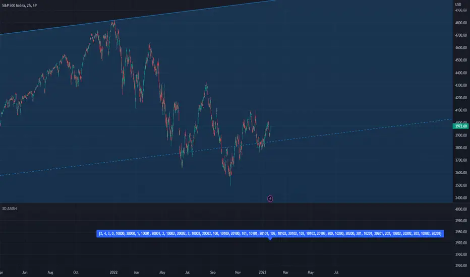
Two Box TheoryA channel is where the price action travels between two rectangular boxes. The Purple box line is treated as resistance and the Blue box line is treated as support.
Two Box Theory is a TradingView TM indicator that automatically locates and prints key support and resistance levels.
Its responsibility lies in its capacity to offer real-time visualisation to support your trade.
It is a flexible indicator that can be used for short or long time frames and has a precision of 8 decimal points, making it appropriate for all types of markets.
You can choose to get alerts immediately because each condition has its own set of alerts.
Two Box Theory has been tried, true, and tested for more than a year and has already earned the faith of those who have used it.
Two Box Theory has what it takes to take your trading to the next level, whether it's used as a stand-alone method or as an addition to your current approach.
Read the description to better understand the functions of this indicator.
1- It will automatically find Pivot Points to determine support and resistance by calculating extensive amount of data.
2- When it calculates new Pivot Points it will remove previous ones and the support/resistance channels will be updated.
3- For every upcoming Pivot Point it scans all previous Pivot Points in its channel horizontally.
4- It will show a different box (grey) when price action goes sideways. This is when the coin is in a no trade zone.
5- After breaking that level(grey box) upwards, it will change colour of its box to make support channel.
6- It will also alert you when the support or resistance breaks, you can set the alerts in the settings.
7- It also includes two Simple Moving Averages for further confirmations.
Here are some screenshots to understand how it functions:
The Auto-Support/Resistance feature in this indicator uses Artificial Intelligence (AI) to automatically plot the support/resistance levels and show them based on the strength of different levels to perform analysis.
AI is used to detect the support/resistance levels and rated based on the following factors:
i- Number of touches
ii- Length of the line
iii- Recency of the line
iv- Violations of the line
You can manage risk according to the support and resistance to set Stop-Loss and the potential take-profit based on the nearest support/resistance levels
Stop loss and take profit levels are made easy on this indicator and if you follow the instructions properly, your accuracy rate should lie between 85-95%
For example:
Support indications:
Resistance Indications and trading technique:
Resistance convert into support:
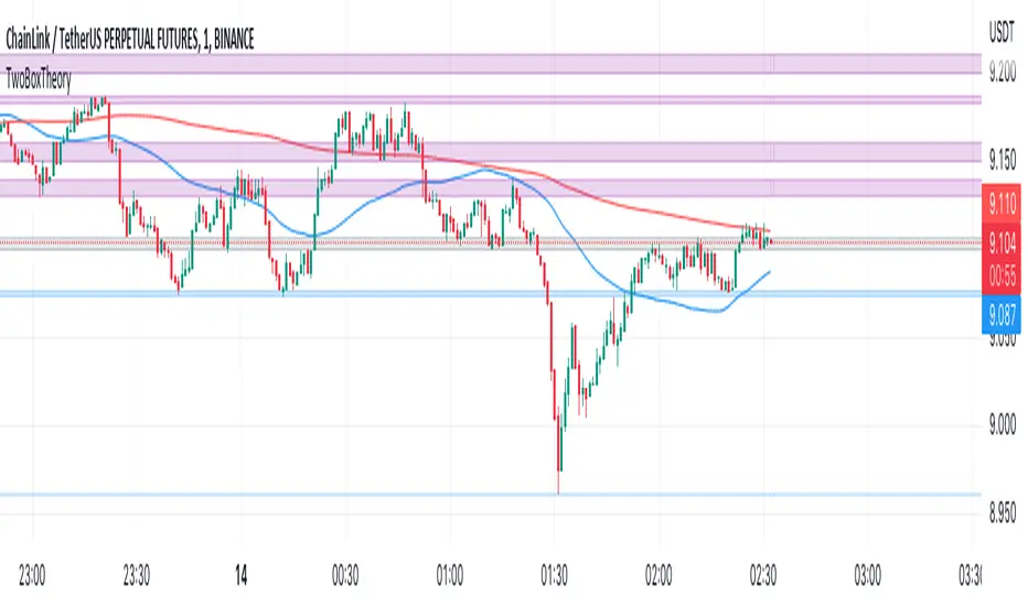
Lune Market Analysis Premium- Version 0.9 -
Lune Algo was developed and built by Lune Trading, utilizing years of their trading expertise. This indicator works on all stocks, cryptos, indices, forex, futures , currencies, ETF's, energy and commodities. All the tools and features you need to assist you on your trading journey. Best of all, Lune Algo is easy to use and many of our tools and strategies have been thoroughly backtested thousands of times to ensure that users have the best experience possible.
Overview
Trade Dashboard—Provides information about the current market conditions, Such as if the market is trending up or down, how much volatility is in the market and even displays information about the current signal.
Trade Statistics—This tool gives you a breakdown of the Statistics of the current selected strategy based on backtests. It tells you the percentage of how often a Take Profit or Stop Loss was hit within a specific time period. Risk and Trade management is very important in trading, and can be the difference between a winning and losing strategy. So we believe that this was mandatory.
Current Features:
Advanced Buy and Sell Signals
Exclusive built-in Strategies
Lune Confidence AI
EK Clouds
Reversal Bands
Vray (Volume Ray)
Divergence Signals
Reversal Signals
Support/Resistance Zones
Built-in Themes
Built-in Risk Management system (take profit/stop loss)
Trade Statistics
Trade Assistance
Trade Dashboard
Advanced Settings
+ More coming soon, Big plans!
Features Breakdown:
Lune Confirmation—Used to help you confirm your trades and trend direction. It uses unique calculations, and its settings can be adjusted to allow traders to adapt the settings to fit their trading style.
Lune Confidence AI—All strategies are equipped with our exclusive built-in Confidence AI. This feature tells you how much confluence there is in a trade. It uses a rating system where signals are given a number from 0 to 5. A rating of 0 indicates that there is not a lot of confluence or confidence in the signal, while a rating of 5 indicates that there is a lot of confidence in the trade. This feature is not perfect and will be improved overtime.
Support/Resistance Zones—Calculates the most important support/resistance levels based on how many times a level has been used as support or resistance. Traders also refer to these as supply and demand zones and key levels.
EK Clouds—Used to further help you confirm trend and was optimized to also be used as support and resistance. This feature is powered by custom moving averages.
Reversal Bands—An optimized and improved version of the infamous Bollinger Bands. When price action takes place within the Reversal Bands it usually indicates that the current symbol is overextended and a reversal is possible.
Vray—Also Known as "Volume Ray", Assists you in better visualizing volume. This helps you find key levels and areas of support that you wouldn't be able to see otherwise. It helps you trade like the institutions.
This indicator's signals DO NOT REPAINT.
If you are using this script you acknowledge past performance is not necessarily indicative of future results and there are many more factors that go into being a profitable trader.
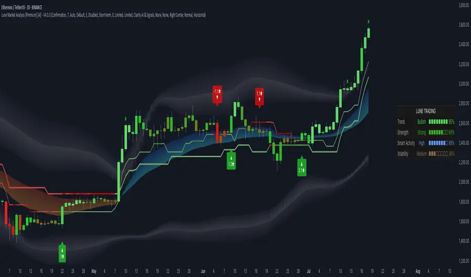
Volume Spike Strategy This is a Pine Script implementation of “Capitalize AI: Volume Spike Strategy" by Bitcoin Trading Challenge (copied with permission).
Original Capital AI formula :
If BTC/USD 1 minute volume > BTC/USD average volume in 20-1m bar by at least 500% and if BTC/USD is below the MA (5,1m,close) of BTC/USD then buy 10,000 USD WORTH of BTC/USD
Tested on XBTUSD 1 minute.
Original strategy is buy-only. Option for sells was added (enable in settings).
First published script -- comments/feedback appreciated
ADX DMI 3x - Dingue- ADX DMI DINGUE -
Français (bottom) / English
The best baddest - The Ultimate ADX DMI indicator for you to use.
Good to clearly see who's in control. Bear Bull
Includes :
- 3x ADX
- 3x DMI
- 3 line system which uses DMI calculation and put it in a single line instead of positive / negative.
Manual or Auto settings which adjusts length based on time frame used on screen.
Color coded for clear direction.
Squeeze shows when both sides are close together and this is when the trend might change or keep going.
Suggestions are welcome, ask below for any questions.
Try my other "DINGUE" indicators.
Thanks.
----------------- Français -----------------
Le meilleur, le plus génial - L'ultime indicateur ADX DMI pour votre utilisation
Très bon pour voir qui est en contrôle.
Inclu :
- 3x ADX
- 3x DMI
- 3 lignes qui remplace les lignes positives négatives du DMI pour une visualisation plus simple.
Paramétrage manuel ou automatique qui ajuste les valeurs selon la grandeur de chandelles utilisée à l'écran.
Codé avec des couleurs pour une visibilités de la direction claire.
Squeeze qui montre quand les 2 côtés sont près l'un de l'autre et quand un changement de contrôle ou une continuation de la tendance se produit.
Suggestions appréciées, pour toutes questions, écrire dans les commentaires plus bas.
Essayez les autres indicateurs "DINGUE".
Merci.