Friendly IT Algo System_2026Friendly IT Algo System V1 is a comprehensive trend-following system that combines SMC (Smart Money Concepts) order blocks with powerful volume filters.
🧠 Key Features:
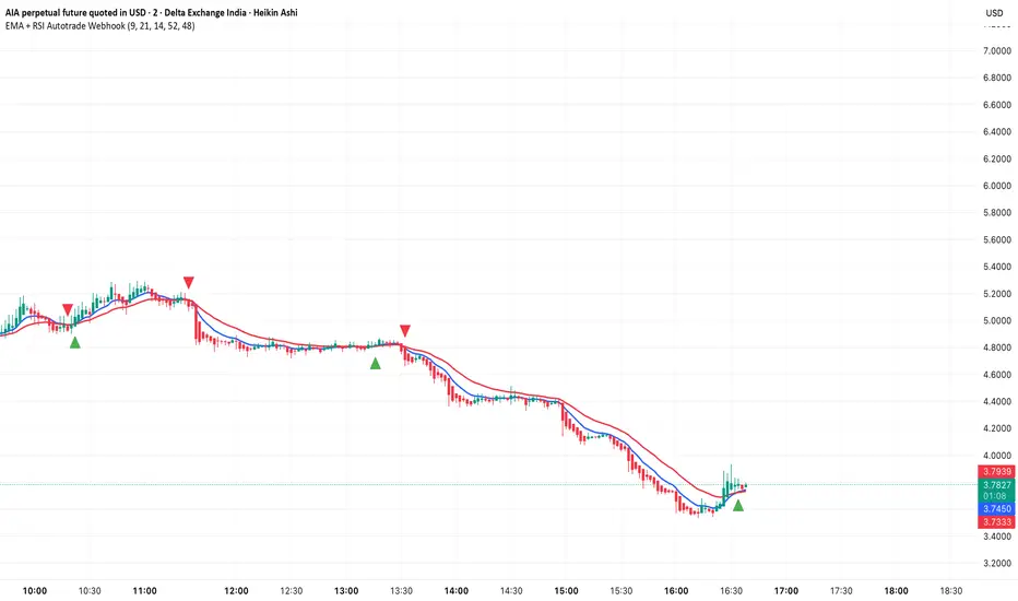
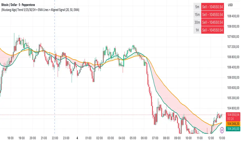
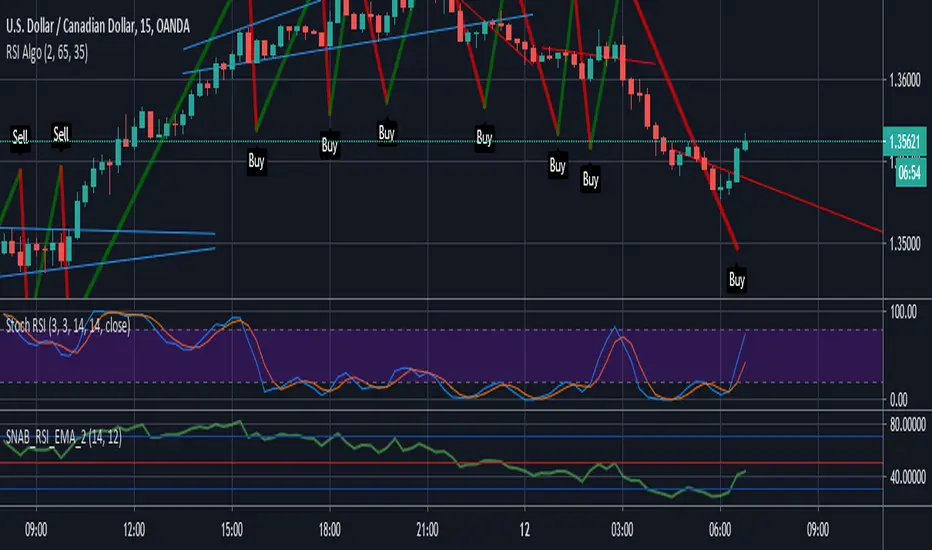
Smart Trend Signals: EMA 7/20 crossover filtered by market energy.
SMC Order Blocks: Automated key supply/demand zones.
Regular Divergence: RSI-based trend reversal tracking.
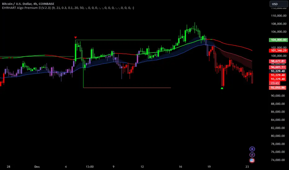
Auto Fib & Pivot: Displays 0.618 golden level and pivot S/R.
Sideways Filter: ADX-based gray background to avoid choppy markets.
Penunjuk Pine Script®