Dresteghamat-Multi timeframe Regime & Exhaustion**Dresteghamat-Multi timeframe Regime & Exhaustion**
This script is a custom decision-support dashboard that aggregates volatility, momentum, and structural data across multiple timeframes to filter market noise. It addresses the problem of "Analysis Paralysis" by automating the correlation between lower timeframe momentum and higher timeframe structure using a weighted scoring algorithm.
### 🔧 Methodology & Calculation Logic
The core engine does not simply overlay indicators; it normalizes their outputs into a unified score (-100 to +100). The logic is hidden (Protected) to preserve the proprietary weighting algorithm, but the underlying concepts are as follows:
**1. Adaptive Timeframe Selection (Context Engine)**
Instead of static monitoring, the script detects the user's current chart timeframe (`timeframe.multiplier`) and dynamically assigns two relevant Higher Timeframes (HTF) as anchors.
* *Logic:* If Current TF < 5min, the script analyzes 15m and 1H data. If Current TF < 1H, it shifts to 4H and Daily data. This ensures the analysis is contextually relevant.
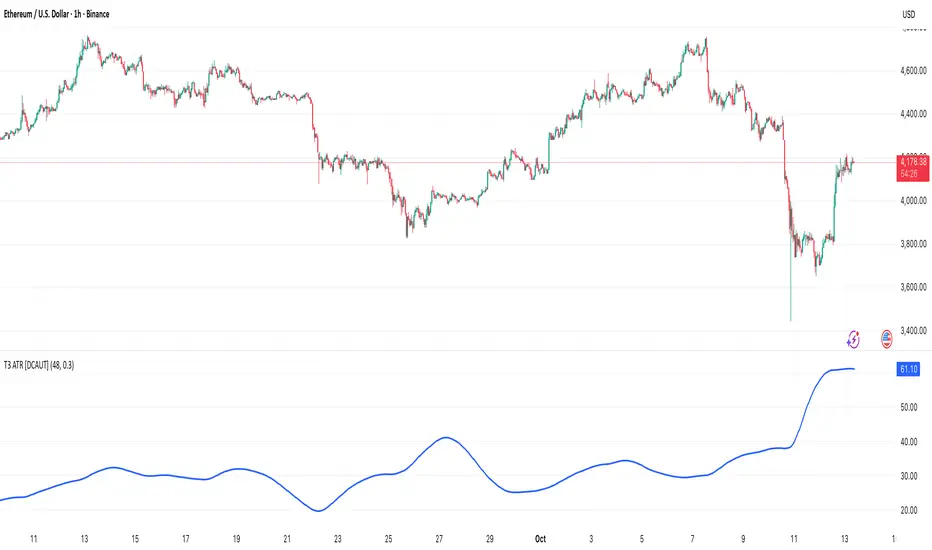
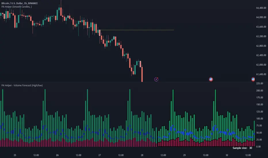
**2. Regime & Volatility Filter (ATR Based)**
We use the Average True Range (ATR) to determine the market regime (Trend vs. Range).
* **Calculation:** We compare the current Swing Range (High-Low lookback) against a smoothed ATR. A high Ratio (> 2.0) indicates a Trend Regime, activating Trend-Following logic. A low ratio dampens the signals.
**3. Directional Bias (Structure + Flow)**
Direction is not determined by a single crossover. It is a fusion of:
* **Swing Structure:** Using `ta.pivothigh/low` to identify Higher Highs/Lower Lows.
* **Volume Flow:** Calculating the cumulative delta of candle bodies over a lookback period.
* **Micro-Bias:** A short-term (default 5-bar) momentum filter to detect immediate order flow changes.
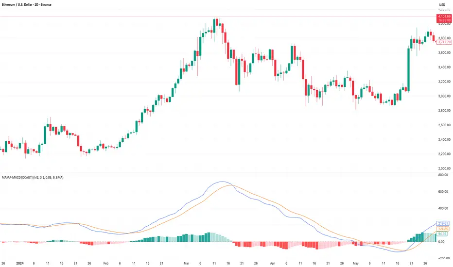
**4. Exhaustion Logic (Mean Reversion Warning)**
To prevent buying at tops, the script calculates an "Exhaustion Score" based on:
* **RSI Divergence:** Detecting discrepancies between price peaks and momentum.
* **Volatility Extension:** Identifying when price has deviated significantly from its volatility mean (VRSD logic).
* **Volume Anomalies:** Detecting low volume on new highs (Supply absorption).
### 📊 How to Read the Dashboard
The table displays the raw status of each timeframe. The **"MODE"** row is the output of the algorithmic decision tree:
* **BUY/SELL ONLY:** Generated when the Current TF momentum aligns with the dynamically selected HTF structure AND the Exhaustion Score is below the threshold (default 70).
* **PULLBACK:** Triggered when the HTF Structure is bullish, but Current Momentum is bearish (indicating a corrective phase).
* **HTF EXHAUST:** A safety warning triggered when the HTF Volatility or RSI metrics hit extreme levels, overriding any entry signals.
* **WAIT:** Default state when volatility is low (Range Regime) or signals conflict.
### ⚠️ Disclaimer
This tool provides algorithmic analysis based on historical price action and volatility metrics. It does not guarantee future results.
Penunjuk Pine Script®