Ratings AlgoThe ratings algo is my discount version of the many paid-for algorithms put out by numerous different companies. A technical "rating" (by default between -10 and 10) is produced for each candle, telling the user when to buy, sell, or hold. I took 11 of my personal favorite indicators to develop a rating system. They are:
50/200 SMA crossover
10/20 SMA crossover
10/20 LSMA crossover
10/20 EMA crossover
"Arnold" a rate-of-change analysis of a smoothed LSMA
PVT and OBV momentum
MACD
RSI
DMI
Fisher Transform
The ratings system is very basic (a more complex, detailed version will be coming in the future!) where each indicator returns -1, 0, or 1, and the MAs and Oscillators are stratified with a user-defined weighting. The total calculation is based on the function:
maweight * (average of MA ratings) + oscillator weight * (average of osc ratings)
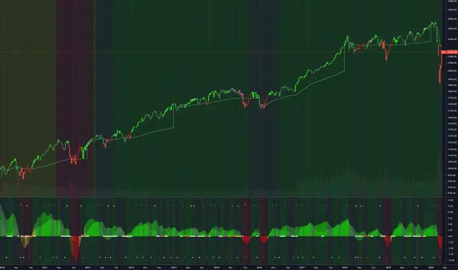
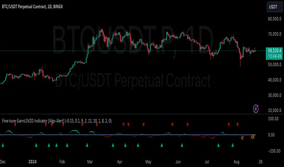
If the total value > user-defined threshold, the bar is teal, and if > 2.5 * threshold, is green, and vice versa for orange/red respectively. Purple is given if the total value is close to zero.
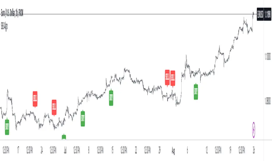
"Strong" signals are printed if the bar changes to either green or red and exits are printed if the bars change from green/red to any other color.
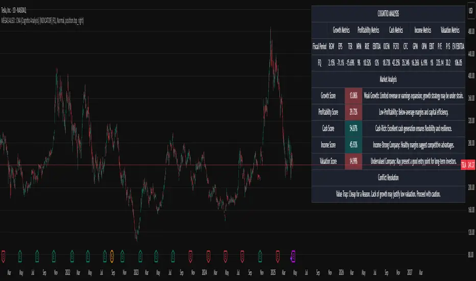
A table is also produced showing what each indicator is indicating, either "Buy" "Sell" or "Hold.
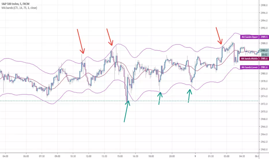
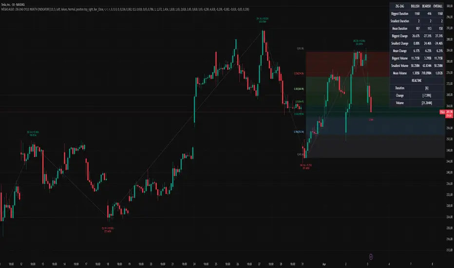
Reversal Bands are printed, intended to be used as areas where a trade might be exited if the market is sideways. If a Strong Buy signal is produced, it may be a good idea to enter the trade, and hold until the price enters the reversal bands, then hold until a candle closes outside the band for the first time.
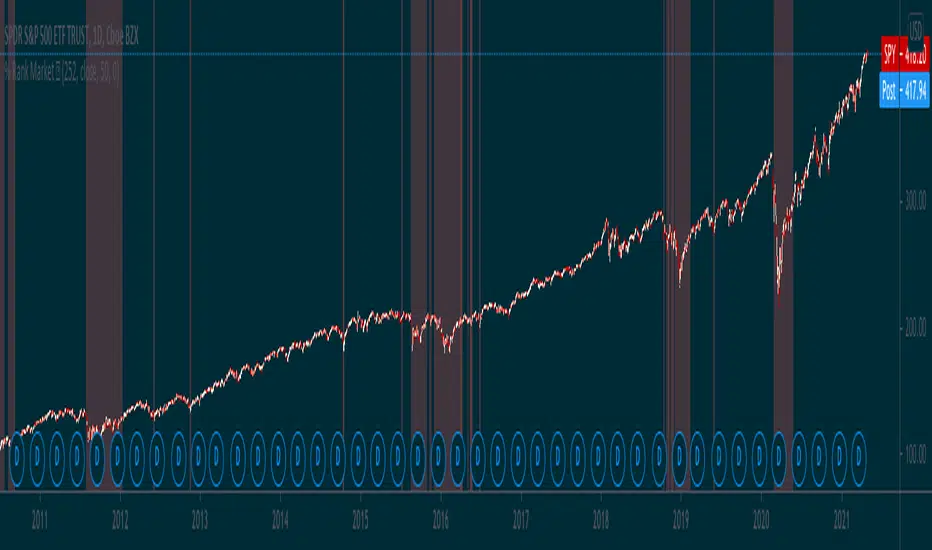
This indicator truly shines in trending markets (like most indicators), but with very fast-acting exit signals and reversal zones, will facilitate minimal losses and possibly even profits in sideways markets.
Penunjuk Pine Script®