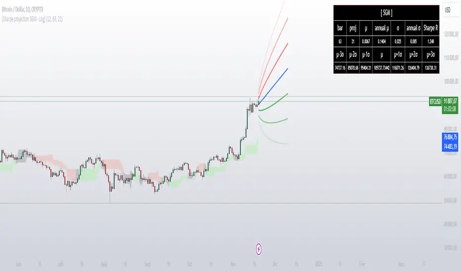
[Sharpe projection SGM]Dynamic Support and Resistance: Traces adjustable support and resistance lines based on historical prices, signaling new market barriers.
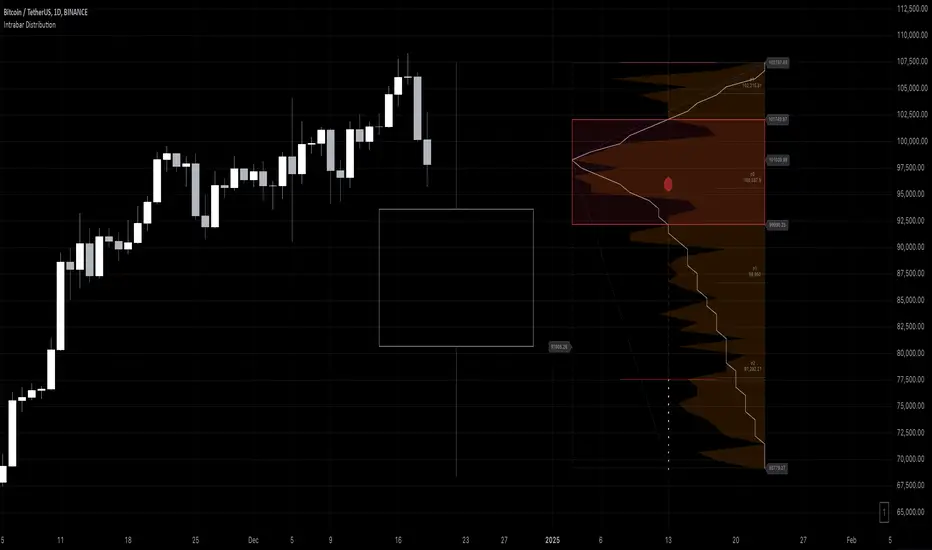
Price Projections and Volatility: Calculates future price projections using moving averages and plots annualized standard deviation-based volatility bands to anticipate price dispersion.
Intuitive Coloring: Colors between support and resistance lines show up or down trends, making it easy to analyze quickly.
Analytics Dashboard: Displays key metrics such as the Sharpe Ratio, which measures average ROI adjusted for asset volatility
Volatility Management for Options Trading: The script helps evaluate strike prices and strategies for options, based on support and resistance levels and projected volatility.
Importance of Diversification: It is necessary to diversify investments to reduce risks and stabilize returns.
Disclaimer on Past Performance: Past performance does not guarantee future results, projections should be supplemented with other analyses.
The script settings can be adjusted according to the specific needs of each user.
The mean and standard deviation are two fundamental statistical concepts often represented in a Gaussian curve, or normal distribution. Here's a quick little lesson on these concepts:
Average
The mean (or arithmetic mean) is the result of the sum of all values in a data set divided by the total number of values. In a data distribution, it represents the center of gravity of the data points.
Standard Deviation
The standard deviation measures the dispersion of the data relative to its mean. A low standard deviation indicates that the data is clustered near the mean, while a high standard deviation shows that it is more spread out.
Gaussian curve
The Gaussian curve or normal distribution is a graphical representation showing the probability of distribution of data. It has the shape of a symmetrical bell centered on the middle. The width of the curve is determined by the standard deviation.
68-95-99.7 rule (rule of thumb): Approximately 68% of the data is within one standard deviation of the mean, 95% is within two standard deviations, and 99.7% is within three standard deviations.
In statistics, understanding the mean and standard deviation allows you to infer a lot about the nature of the data and its trends, and the Gaussian curve provides an intuitive visualization of this information.
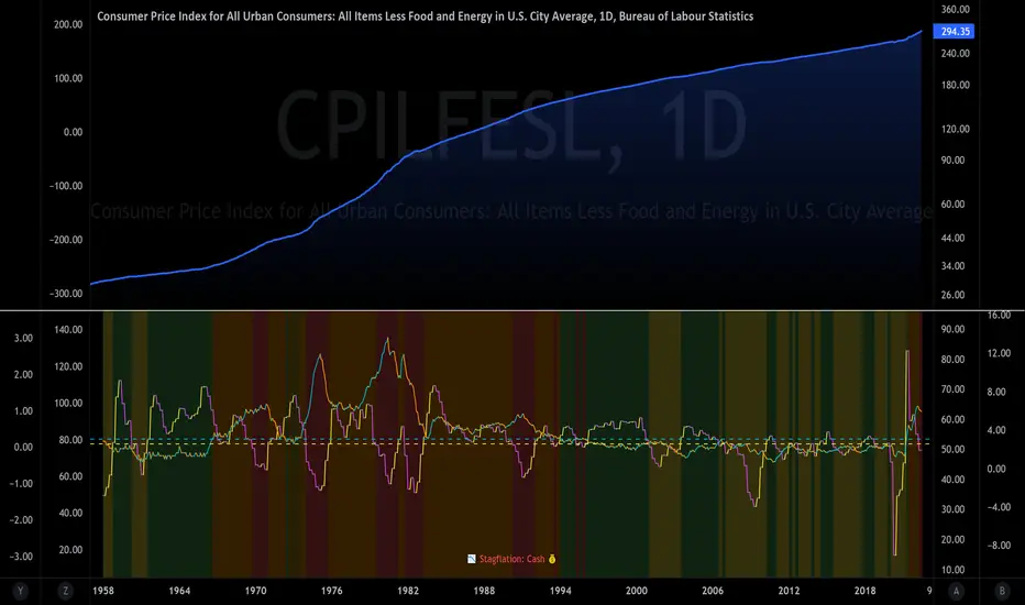
In finance, it is crucial to remember that data dispersion can be more random and unpredictable than traditional statistical models like the normal distribution suggest. Financial markets are often affected by unforeseen events or changes in investor behavior, which can result in return distributions with wider standard deviations or non-symmetrical distributions.
Penunjuk Pine Script®