VWAP For Loop [BackQuant]VWAP For Loop
What this tool does—in one sentence
A volume-weighted trend gauge that anchors VWAP to a calendar period (day/week/month/quarter/year) and then scores the persistence of that VWAP trend with a simple for-loop “breadth” count; the result is a clean, threshold-driven oscillator plus an optional VWAP overlay and alerts.
Plain-English overview
Instead of judging raw price alone, this indicator focuses on anchored VWAP —the market’s average price paid during your chosen institutional period. It then asks a simple question across a configurable set of lookback steps: “Is the current anchored VWAP higher than it was i bars ago—or lower?” Each “yes” adds +1, each “no” adds −1. Summing those answers creates a score that reflects how consistently the volume-weighted trend has been rising or falling. Extreme positive scores imply persistent, broad strength; deeply negative scores imply persistent weakness. Crossing predefined thresholds produces objective long/short events and color-coded context.
Under the hood
• Anchoring — VWAP using hlc3 × volume resets exactly when the selected period rolls:
Day → session change, Week → new week, Month → new month, Quarter/Year → calendar quarter/year.
• For-loop scoring — For lag steps i = , compare today’s VWAP to VWAP .
– If VWAP > VWAP , add +1.
– Else, add −1.
The final score ∈ , where N = (end − start + 1). With defaults (1→45), N = 45.
• Signal logic (stateful)
– Long when score > upper (e.g., > 40 with N = 45 → VWAP higher than ~89% of checked lags).
– Short on crossunder of lower (e.g., dropping below −10).
– A compact state variable ( out ) holds the current regime: +1 (long), −1 (short), otherwise unchanged. This “stickiness” avoids constant flipping between bars without sufficient evidence.
Why VWAP + a breadth score?
• VWAP aggregates both price and volume—where participants actually traded.
• The breadth-style count rewards consistency of the anchored trend, not one-off spikes.
• Thresholds give you binary structure when you need it (alerts, automation), without complex math.
What you’ll see on the chart
• Sub-pane oscillator — The for-loop score line, colored by regime (long/short/neutral).
• Main-pane VWAP (optional) — Even though the indicator runs off-chart, the anchored VWAP can be overlaid on price (toggle visibility and whether it inherits trend colors).
• Threshold guides — Horizontal lines for the long/short bands (toggle).
• Cosmetics — Optional candle painting and background shading by regime; adjustable line width and colors.
Input map (quick reference)
• VWAP Anchor Period — Day, Week, Month, Quarter, Year.
• Calculation Start/End — The for-loop lag window . With 1→45, you evaluate 45 comparisons.
• Long/Short Thresholds — Default upper=40, lower=−10 (asymmetric by design; see below).
• UI/Style — Show thresholds, paint candles, background color, line width, VWAP visibility and coloring, custom long/short colors.
Interpreting the score
• Near +N — Current anchored VWAP is above most historical VWAP checkpoints in the window → entrenched strength.
• Near −N — Current anchored VWAP is below most checkpoints → entrenched weakness.
• Between — Mixed, choppy, or transitioning regimes; use thresholds to avoid reacting to noise.
Why the asymmetric default thresholds?
• Long = score > upper (40) — Demands unusually broad upside persistence before declaring “long regime.”
• Short = crossunder lower (−10) — Triggers only on downward momentum events (a fresh breach), not merely being below −10. This combination tends to:
– Capture sustained uptrends only when they’re very strong.
– Flag downside turns as they occur, rather than waiting for an extreme negative breadth.
Tuning guide
Choose an anchor that matches your horizon
– Intraday scalps : Day anchor on intraday charts.
– Swing/position : Month or Quarter anchor on 1h/4h/D charts to capture institutional cycles.
Pick the for-loop window
– Larger N (bigger end) = stronger evidence requirement, smoother oscillator.
– Smaller N = faster, more reactive score.
Set achievable thresholds
– Ensure upper ≤ N and lower ≥ −N ; if N=30, an upper of 40 can never trigger.
– Symmetric setups (e.g., +20/−20) are fine if you want balanced behavior.
Match visuals to intent
– Enabling VWAP coloring lets you see regime directly on price.
– Background shading is useful for discretionary reading; turn it off for cleaner automation displays.
Playbook examples
• Trend confirmation with disciplined entries — On Month anchor, N=45, upper=38–42: when the long regime engages, use pullbacks toward anchored VWAP on the main pane for entries, with stops just beyond VWAP or a recent swing.
• Downside transition detection — Keep lower around −8…−12 and watch for crossunders; combine with price losing anchored VWAP to validate risk-off.
• Intraday bias filter — Day anchor on a 5–15m chart, N=20–30, upper ~ 16–20, lower ~ −6…−10. Only take longs while score is positive and above a midline you define (e.g., 0), and shorts only after a genuine crossunder.
Behavior around resets (important)
Anchored VWAP is hard-reset each period. Immediately after a reset, the series can be young and comparisons to pre-reset values may span two periods. If you prefer within-period evaluation only, choose end small enough not to bridge typical period length on your timeframe, or accept that the breadth test intentionally spans regimes.
Alerts included
• VWAP FL Long — Fires when the long condition is true (score > upper and not in short).
• VWAP FL Short — Fires on crossunder of the lower threshold (event-driven).
Messages include {{ticker}} and {{interval}} placeholders for routing.
Strengths
• Simple, transparent math — Easy to reason about and validate.
• Volume-aware by construction — Decisions reference VWAP, not just price.
• Robust to single-bar noise — Needs many lags to agree before flipping state (by design, via thresholds and the stateful output).
Limitations & cautions
• Threshold feasibility — If N < upper or |lower| > N, signals will never trigger; always cross-check N.
• Path dependence — The state variable persists until a new event; if you want frequent re-evaluation, lower thresholds or reduce N.
• Regime changes — Calendar resets can produce early ambiguity; expect a few bars for the breadth to mature.
• VWAP sensitivity to volume spikes — Large prints can tilt VWAP abruptly; that behavior is intentional in VWAP-based logic.
Suggested starting profiles
• Intraday trend bias : Anchor=Day, N=25 (1→25), upper=18–20, lower=−8, paint candles ON.
• Swing bias : Anchor=Month, N=45 (1→45), upper=38–42, lower=−10, VWAP coloring ON, background OFF.
• Balanced reactivity : Anchor=Week, N=30 (1→30), upper=20–22, lower=−10…−12, symmetric if desired.
Implementation notes
• The indicator runs in a separate pane (oscillator), but VWAP itself is drawn on price using forced overlay so you can see interactions (touches, reclaim/loss).
• HLC3 is used for VWAP price; that’s a common choice to dampen wick noise while still reflecting intrabar range.
• For-loop cap is kept modest (≤50) for performance and clarity.
How to use this responsibly
Treat the oscillator as a bias and persistence meter . Combine it with your entry framework (structure breaks, liquidity zones, higher-timeframe context) and risk controls. The design emphasizes clarity over complexity—its edge is in how strictly it demands agreement before declaring a regime, not in predicting specific turns.
Summary
VWAP For Loop distills the question “How broadly is the anchored, volume-weighted trend advancing or retreating?” into a single, thresholded score you can read at a glance, alert on, and color through your chart. With careful anchoring and thresholds sized to your window length, it becomes a pragmatic bias filter for both systematic and discretionary workflows.
Cari dalam skrip untuk "liquidity"
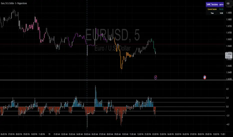
samc's - Keltner OscillatorThe KELTNER CHANNEL is a widely used technical indicator developed in the 60's by Chester W. Keltner who described it in his 1960 book How To Make Money in Commodities.
so i took the logic, simplified the code and made into an oscillator.
to add a flavor of modern times you can choose among 10 different colorways themes in the settings. (so traders can adjust it for dark or light charts)
Although the initial idea was developed for stocks and commodities, I've carefully back tested this as an oscillator across FX MAJORS , MINORS and high liquidity stocks for the use case of scalping and Medium term trade ideas.
now, this indicator works successfully over all time frames, custom time frames and all assets.
This script builds on the same approach as my earlier session tool — keeping things clean, visual, and easy to read.
I intend to publish more of my work as i develop them from Beta ideas into stable scripts, and i welcome feedback.
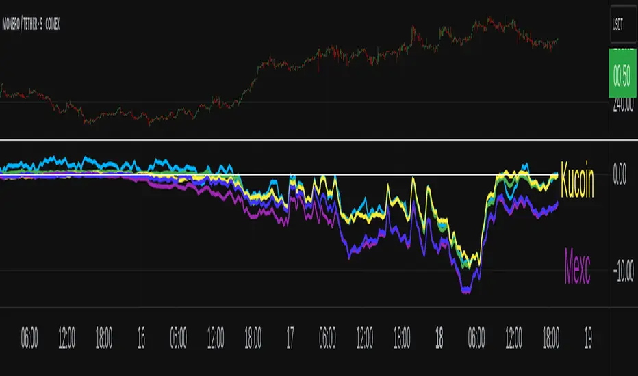
XMR Divergences vs KrakenSUMMARY
This script finds the percentage difference between Kraken, and multiple other exchanges, for the price of XMRUSD, and then runs a variable length moving average of those differences. Optionally, you can multiply by the reported volume of the exchange in question. Skip to "USAGE" at the bottom for a quick view of the settings. But I recommend reading DETAILED DESCRIPTION as well.
PURPOSE
The purpose of this script is to get a look into the relative funds flows of XMR between Kraken and the other exchanges. So long as an exchange withdraws are open: 1) Negative divergences indicate XMR outflows from the exchange under consideration, 2) Postive divergences indicate XMR inflows from Kraken to the exchange.
This appears to be moderately correlated with price movements in Monero (but not always). There is also the theory that positive accumulation is a leading indication of a growing probability of postive price action in the general crypto market, and negative accumulation is a leading indicator of an upcoming peak. In other words, exchanges like to accumulate Monero quietly during calm downtimes, and they like to manage its price from gaining too much attention (pump) during broad market positivity.
BACKGROUND
It's well known among XMR traders that most exchanges are operating on a heavy fractional reserve basis as regards Monero. The past 2 years have seen regular and repeated withdraw freezes, sometimes for weeks/months at a time. Occasionally, liquidity stress tests have been performed, with predictable results - none of these exchanges are able to continue supporting withdraws.
Kraken is the only exchange of meaningful volume that has never frozen withdraws for more than an hour or so. Thus, we theorize that Kraken is operating with all, or most of the XMR they claim to have.
Furthermore, we have seen in the past, large price negative price divergences of these fractional reserve exchanges relative to Kraken. As the social outcry grew stronger for this malfeasance, these exchanges have gone to greater lengths to hide their price divergences.
On minute-by-minute ; hour-by-hour basis, typically, a look with the naked eye would show oscillation around the zero point. But when you average it out, especially on lower timeframes (like the 1 and 5 min candles), you can very clearly see that when withdraws are shut down, these exchanges simultaneously diverge their prices downwards as well.
DETAILED DESCRIPTION
The ideal view of price divergence would compare second-by-second prices, and then run something like a rolling 4-hr or 1-day SMA to average out the overall divergences. However, due to limitations of TradingView, this is impractical/impossible for actual usage/viewing. As a result, a balance must be struck, when selecting the combination of the candle period, and the SMA lookback length.
I find that 5min candles, with a 48-period lookback (that equates to a rolling 4-hour SMA), offers the best view of recent and historical price divergence activity. This of course means that we're only sampling price divergences once every 5 minutes, but it still provides a decent look at what's happening. If this script gets popular, I wouldn't be surprised if these exchanges start timing their candle closes to mask their misdeeds, but that's of course speculative on my part.
The other important factor here, *IS TO MULTIPLY BY VOLUME*. Some of these no-volume exchanges have large price divergences. But if they're not doing any real volume, then it doesn't really have any real market impact. Thus, I recommend keeping the "Make volume adjustment" option on.
If that ends up happening, we'll have to infer that by comparing the difference in close prices, vs the difference in the highest or lowest intra-candle prices (wicks). Typically a divergence should have all 3 showing similar results.
Notes regarding "Sum_of_All": This only makes sense when multiplying by volume. So only check this if you also made the volume adjustment. Generally I believe that *Binance* sets the tone. However, we have seen numerous occasions where Binance diverges down, and the others diverge up. I believe this is a social influence tactic, since most people look at Binance price. Meanwhile, they're trying to accumulate some small amount on the other exchanges to minimize their overall loss. This of course assumes collusion by these exchanges, which is a high likely hood, seeing as how in May 2021, they all diverged together simultaneously (among other evidence).
USAGE
I recommend using your browser zoom, to see data beyond 1 month in the past.
Lookback - The number of candles over which to conduct a moving average. On 5-min candles for example, here's how the math works out:
12 - Equates to a 1 hr MA
24 - 2 hrs
48 - 4 hrs (default)
288 - 1 day
2880 - 10 days
Make Volume Adjustment - Recommend that you usually keep this on.
Line Widths - Set to preference
Show_Close_Price? - You can compute the difference at candle close. Or you can check the other boxes to compare the highest/lowest prices for intra candle prices (wicks).
Show Sum_of_All? - You can sum all of the differences, which only makes sense if you're making the volume adjustement. Default is off. Below, you can also choose which exchanges to include in the sum.
This works best on lower timeframes, like the 1m, 5, and 15m charts. I personally use 5m, with 48 or 96 length lookback. You get a better view of the real time price divergences that way.
Long & Short Liquidations [Kodeus]The Long & Short Liquidations indicator is designed to highlight potential liquidation zones by tracking deviations between short-term and long-term moving averages. It visually emphasizes bullish and bearish extremes while also displaying live volume statistics to help traders gauge market dominance.
This tool aims to provide insights into liquidation pressure, trend signals, and volume dynamics all in one place, assisting traders in identifying possible reversal or continuation points.
🔷 Key Features
Customizable Price Source : Choose between Close, Open, High, or Low as the calculation basis.
Dual Moving Average Baseline : Uses a combination of SMA (fast) and EMA (slow) for deviation tracking.
Liquidation Peaks : Detects bullish and bearish extremes, plotting signals where strong deviations occur.
Real-Time Volume Stats: Displays bull and bear volume, ratio, and market dominance in a compact table.
🔷 Disclaimer
Use with Caution: This indicator is provided for educational and informational purposes only and should not be considered as financial advice. Users should exercise caution and perform their own analysis before making trading decisions based on the indicator's signals.
Not Financial Advice: The information provided by this indicator does not constitute financial advice, and the creator shall not be held responsible for any trading losses incurred as a result of using this indicator.
Backtesting Recommended: Traders are encouraged to backtest the indicator thoroughly on historical data before using it in live trading to assess its performance and suitability for their trading strategies.
Risk Management: Trading involves inherent risks, and users should implement proper risk management strategies, including but not limited to stop-loss orders and position sizing, to mitigate potential losses.
No Guarantees: The accuracy and reliability of the indicator's signals cannot be guaranteed, as they are based on historical price data and past performance may not be indicative of future results.

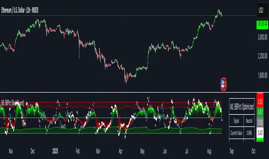
Machine Learning BBPct [BackQuant]Machine Learning BBPct
What this is (in one line)
A Bollinger Band %B oscillator enhanced with a simplified K-Nearest Neighbors (KNN) pattern matcher. The model compares today’s context (volatility, momentum, volume, and position inside the bands) to similar situations in recent history and blends that historical consensus back into the raw %B to reduce noise and improve context awareness. It is informational and diagnostic—designed to describe market state, not to sell a trading system.
Background: %B in plain terms
Bollinger %B measures where price sits inside its dynamic envelope: 0 at the lower band, 1 at the upper band, ~ 0.5 near the basis (the moving average). Readings toward 1 indicate pressure near the envelope’s upper edge (often strength or stretch), while readings toward 0 indicate pressure near the lower edge (often weakness or stretch). Because bands adapt to volatility, %B is naturally comparable across regimes.
Why add (simplified) KNN?
Classic %B is reactive and can be whippy in fast regimes. The simplified KNN layer builds a “nearest-neighbor memory” of recent market states and asks: “When the market looked like this before, where did %B tend to be next bar?” It then blends that estimate with the current %B. Key ideas:
• Feature vector . Each bar is summarized by up to five normalized features:
– %B itself (normalized)
– Band width (volatility proxy)
– Price momentum (ROC)
– Volume momentum (ROC of volume)
– Price position within the bands
• Distance metric . Euclidean distance ranks the most similar recent bars.
• Prediction . Average the neighbors’ prior %B (lagged to avoid lookahead), inverse-weighted by distance.
• Blend . Linearly combine raw %B and KNN-predicted %B with a configurable weight; optional filtering then adapts to confidence.
This remains “simplified” KNN: no training/validation split, no KD-trees, no scaling beyond windowed min-max, and no probabilistic calibration.
How the script is organized (by input groups)
1) BBPct Settings
• Price Source – Which price to evaluate (%B is computed from this).
• Calculation Period – Lookback for SMA basis and standard deviation.
• Multiplier – Standard deviation width (e.g., 2.0).
• Apply Smoothing / Type / Length – Optional smoothing of the %B stream before ML (EMA, RMA, DEMA, TEMA, LINREG, HMA, etc.). Turning this off gives you the raw %B.
2) Thresholds
• Overbought/Oversold – Default 0.8 / 0.2 (inside ).
• Extreme OB/OS – Stricter zones (e.g., 0.95 / 0.05) to flag stretch conditions.
3) KNN Machine Learning
• Enable KNN – Switch between pure %B and hybrid.
• K (neighbors) – How many historical analogs to blend (default 8).
• Historical Period – Size of the search window for neighbors.
• ML Weight – Blend between raw %B and KNN estimate.
• Number of Features – Use 2–5 features; higher counts add context but raise the risk of overfitting in short windows.
4) Filtering
• Method – None, Adaptive, Kalman-style (first-order),
or Hull smoothing.
• Strength – How aggressively to smooth. “Adaptive” uses model confidence to modulate its alpha: higher confidence → stronger reliance on the ML estimate.
5) Performance Tracking
• Win-rate Period – Simple running score of past signal outcomes based on target/stop/time-out logic (informational, not a robust backtest).
• Early Entry Lookback – Horizon for forecasting a potential threshold cross.
• Profit Target / Stop Loss – Used only by the internal win-rate heuristic.
6) Self-Optimization
• Enable Self-Optimization – Lightweight, rolling comparison of a few canned settings (K = 8/14/21 via simple rules on %B extremes).
• Optimization Window & Stability Threshold – Governs how quickly preferred K changes and how sensitive the overfitting alarm is.
• Adaptive Thresholds – Adjust the OB/OS lines with volatility regime (ATR ratio), widening in calm markets and tightening in turbulent ones (bounded 0.7–0.9 and 0.1–0.3).
7) UI Settings
• Show Table / Zones / ML Prediction / Early Signals – Toggle informational overlays.
• Signal Line Width, Candle Painting, Colors – Visual preferences.
Step-by-step logic
A) Compute %B
Basis = SMA(source, len); dev = stdev(source, len) × multiplier; Upper/Lower = Basis ± dev.
%B = (price − Lower) / (Upper − Lower). Optional smoothing yields standardBB .
B) Build the feature vector
All features are min-max normalized over the KNN window so distances are in comparable units. Features include normalized %B, normalized band width, normalized price ROC, normalized volume ROC, and normalized position within bands. You can limit to the first N features (2–5).
C) Find nearest neighbors
For each bar inside the lookback window, compute the Euclidean distance between current features and that bar’s features. Sort by distance, keep the top K .
D) Predict and blend
Use inverse-distance weights (with a strong cap for near-zero distances) to average neighbors’ prior %B (lagged by one bar). This becomes the KNN estimate. Blend it with raw %B via the ML weight. A variance of neighbor %B around the prediction becomes an uncertainty proxy ; combined with a stability score (how long parameters remain unchanged), it forms mlConfidence ∈ . The Adaptive filter optionally transforms that confidence into a smoothing coefficient.
E) Adaptive thresholds
Volatility regime (ATR(14) divided by its 50-bar SMA) nudges OB/OS thresholds wider or narrower within fixed bounds. The aim: comparable extremeness across regimes.
F) Early entry heuristic
A tiny two-step slope/acceleration probe extrapolates finalBB forward a few bars. If it is on track to cross OB/OS soon (and slope/acceleration agree), it flags an EARLY_BUY/SELL candidate with an internal confidence score. This is explicitly a heuristic—use as an attention cue, not a signal by itself.
G) Informational win-rate
The script keeps a rolling array of trade outcomes derived from signal transitions + rudimentary exits (target/stop/time). The percentage shown is a rough diagnostic , not a validated backtest.
Outputs and visual language
• ML Bollinger %B (finalBB) – The main line after KNN blending and optional filtering.
• Gradient fill – Greenish tones above 0.5, reddish below, with intensity following distance from the midline.
• Adaptive zones – Overbought/oversold and extreme bands; shaded backgrounds appear at extremes.
• ML Prediction (dots) – The KNN estimate plotted as faint circles; becomes bright white when confidence > 0.7.
• Early arrows – Optional small triangles for approaching OB/OS.
• Candle painting – Light green above the midline, light red below (optional).
• Info panel – Current value, signal classification, ML confidence, optimized K, stability, volatility regime, adaptive thresholds, overfitting flag, early-entry status, and total signals processed.
Signal classification (informational)
The indicator does not fire trade commands; it labels state:
• STRONG_BUY / STRONG_SELL – finalBB beyond extreme OS/OB thresholds.
• BUY / SELL – finalBB beyond adaptive OS/OB.
• EARLY_BUY / EARLY_SELL – forecast suggests a near-term cross with decent internal confidence.
• NEUTRAL – between adaptive bands.
Alerts (what you can automate)
• Entering adaptive OB/OS and extreme OB/OS.
• Midline cross (0.5).
• Overfitting detected (frequent parameter flipping).
• Early signals when early confidence > 0.7.
These are purely descriptive triggers around the indicator’s state.
Practical interpretation
• Mean-reversion context – In range markets, adaptive OS/OB with ML smoothing can reduce whipsaws relative to raw %B.
• Trend context – In persistent trends, the KNN blend can keep finalBB nearer the mid/upper region during healthy pullbacks if history supports similar contexts.
• Regime awareness – Watch the volatility regime and adaptive thresholds. If thresholds compress (high vol), “OB/OS” comes sooner; if thresholds widen (calm), it takes more stretch to flag.
• Confidence as a weight – High mlConfidence implies neighbors agree; you may rely more on the ML curve. Low confidence argues for de-emphasizing ML and leaning on raw %B or other tools.
• Stability score – Rising stability indicates consistent parameter selection and fewer flips; dropping stability hints at a shifting backdrop.
Methodological notes
• Normalization uses rolling min-max over the KNN window. This is simple and scale-agnostic but sensitive to outliers; the distance metric will reflect that.
• Distance is unweighted Euclidean. If you raise featureCount, you increase dimensionality; consider keeping K larger and lookback ample to avoid sparse-neighbor artifacts.
• Lag handling intentionally uses neighbors’ previous %B for prediction to avoid lookahead bias.
• Self-optimization is deliberately modest: it only compares a few canned K/threshold choices using simple “did an extreme anticipate movement?” scoring, then enforces a stability regime and an overfitting guard. It is not a grid search or GA.
• Kalman option is a first-order recursive filter (fixed gain), not a full state-space estimator.
• Hull option derives a dynamic length from 1/strength; it is a convenience smoothing alternative.
Limitations and cautions
• Non-stationarity – Nearest neighbors from the recent window may not represent the future under structural breaks (policy shifts, liquidity shocks).
• Curse of dimensionality – Adding features without sufficient lookback can make genuine neighbors rare.
• Overfitting risk – The script includes a crude overfitting detector (frequent parameter flips) and will fall back to defaults when triggered, but this is only a guardrail.
• Win-rate display – The internal score is illustrative; it does not constitute a tradable backtest.
• Latency vs. smoothness – Smoothing and ML blending reduce noise but add lag; tune to your timeframe and objectives.
Tuning guide
• Short-term scalping – Lower len (10–14), slightly lower multiplier (1.8–2.0), small K (5–8), featureCount 3–4, Adaptive filter ON, moderate strength.
• Swing trading – len (20–30), multiplier ~2.0, K (8–14), featureCount 4–5, Adaptive thresholds ON, filter modest.
• Strong trends – Consider higher adaptive_upper/lower bounds (or let volatility regime do it), keep ML weight moderate so raw %B still reflects surges.
• Chop – Higher ML weight and stronger Adaptive filtering; accept lag in exchange for fewer false extremes.
How to use it responsibly
Treat this as a state descriptor and context filter. Pair it with your execution signals (structure breaks, volume footprints, higher-timeframe bias) and risk management. If mlConfidence is low or stability is falling, lean less on the ML line and more on raw %B or external confirmation.
Summary
Machine Learning BBPct augments a familiar oscillator with a transparent, simplified KNN memory of recent conditions. By blending neighbors’ behavior into %B and adapting thresholds to volatility regime—while exposing confidence, stability, and a plain early-entry heuristic—it provides an informational, probability-minded view of stretch and reversion that you can interpret alongside your own process.
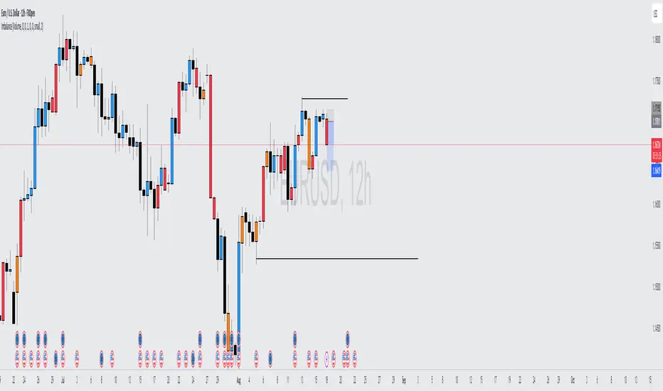
Volume Imbalance Analyzer - 70% & 80% Version1.01Here’s a clean “definition” you can drop into your docs. It explains **what** the indicator is, **what it helps with**, and **how** to use it—plain and practical.
# Definition
**Volume Imbalance Analyzer (70% & 80%)** flags bars where estimated buy vs. sell volume is heavily one-sided. It colors those bars, adds labels (B70/B80 or S70/S80), and can alert you in real time. The goal is to quickly spot spots of **aggressive participation** (buyers or sellers) that often act as magnets for a **retest** or as **exhaustion/continuation** areas.
# What it helps you do
* **Find high-energy bars** where one side dominates (potential turning or continuation points).
* **Plan retests:** Track when price comes back into the imbalance candle’s range (common entry/take-profit logic).
* **Filter trades:** Only act when the market shows unusual pressure (≥70% or ≥80%).
* **Add context to setups:** Combine with S/R, FVGs, or trend tools to time entries with less guesswork.
* **Alert-driven workflow:** Get notified the moment extreme pressure prints.
# How it helps (workflow)
1. **Scan for signals:**
* **B80/B70** = strong buying; **S80/S70** = strong selling.
* 80% is “extreme” and overrides 70%.
2. **Mark the zone:** The imbalance candle’s **high–low** defines a zone. Many traders wait for a **retest** into that range.
3. **Decide intent:**
* After **B80/B70**, look for pullbacks to buy (or fades if you see exhaustion).
* After **S80/S70**, look for rallies to sell (or fades if exhaustion).
4. **Confirm with context:** Check trend, key levels, liquidity, session timing, ATR/volatility.
5. **Manage risk:** Place stops beyond the zone; size trades so a failed retest doesn’t ruin the day.
# How it works (under the hood, briefly)
The script **estimates buy/sell volume** from each candle’s body, wicks, and total volume, then computes an **imbalance %**. If the % crosses **70%** or **80%** (scaled by a Sensitivity setting), it paints the bar, drops a label, and optionally fires an alert. It also stores the imbalance candle’s range so you can watch for a **retest**.
# Reading the signals (quick guide)
* **B80**: Extreme buyer pressure → watch for pullback buys or exhaustion shorts, depending on context.
* **B70**: Strong buyer pressure → mild continuation bias.
* **S80**: Extreme seller pressure → watch for rally sells or exhaustion longs.
* **S70**: Strong seller pressure → higher reversal probability noted in the table (informational).
# Configuration tips
* **Sensitivity**: Higher = more bars qualify (more signals).
* **Label distance**: Scales with ATR so labels don’t overlap candles.
* **Colors/opacity**: Separate for 70% vs 80% and buyer vs seller.
* **Alerts**: Enable to catch signals live without staring at the screen.
# Notes & limits
* Uses **estimation** (not true bid/ask) on most symbols; treat as a **context tool**, not a stand-alone system.
* The optional stats table’s “expected outcomes” are **informational**, not live probabilities.
* Works on any timeframe; results improve when combined with structure and risk controls.
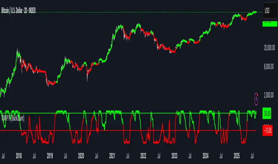
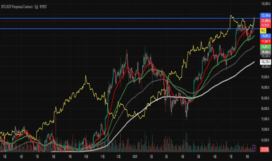
BTC Power Law Valuation BandsBTC Power Law Rainbow
A long-term valuation framework for Bitcoin based on Power Law growth — designed to help identify macro accumulation and distribution zones, aligned with long-term investor behavior.
🔍 What Is a Power Law?
A Power Law is a mathematical relationship where one quantity varies as a power of another. In this model:
Price ≈ a × (Time)^b
It captures the non-linear, exponentially slowing growth of Bitcoin over time. Rather than using linear or cyclical models, this approach aligns with how complex systems, such as networks or monetary adoption curves, often grow — rapidly at first, and then more slowly, but persistently.
🧠 Why Power Law for BTC?
Bitcoin:
Has finite supply and increasing adoption.
Operates as a monetary network , where Metcalfe’s Law and power laws naturally emerge.
Exhibits exponential growth over logarithmic time when viewed on a log-log chart .
This makes it uniquely well-suited for power law modeling.
🌈 How to Use the Valuation Bands
The central white line represents the modeled fair value according to the power law.
Colored bands represent deviations from the model in logarithmic space, acting as macro zones:
🔵 Lower Bands: Deep value / Accumulation zones.
🟡 Mid Bands: Fair value.
🔴 Upper Bands: Euphoria / Risk of macro tops.
📐 Smart Money Concepts (SMC) Alignment
Accumulation: Occurs when price consolidates near lower bands — often aligning with institutional positioning.
Markup: As price re-enters or ascends the bands, we often see breakout behavior and trend expansion.
Distribution: When price extends above upper bands, potential for exit liquidity creation and distribution events.
Reversion: Historically, price mean-reverts toward the model — rarely staying outside the bands for long.
This makes the model useful for:
Cycle timing
Long-term DCA strategy zones
Identifying value dislocations
Filtering short-term noise
⚠️ Disclaimer
This tool is for educational and informational purposes only . It is not financial advice. The power law model is a non-predictive, mathematical framework and does not guarantee future price movements .
Always use additional tools, risk management, and your own judgment before making trading or investment decisions.

VWAP Suite {Phanchai}VWAP Suite {Phanchai}
Compact, readable, TradingView-friendly.
What is VWAP?
The Volume Weighted Average Price (VWAP) is the average price of a period weighted by traded volume. It’s used as a fair-value reference (mean) and resets at the start of each new period.
Included VWAP Modes
Session — resets each trading day (current session).
Week / Month / Quarter / Year — current calendar periods.
Anchored Week / Month / Quarter / Year — starts at the beginning of the previous completed period.
Rolling 7D / 30D / 90D — rolling windows: today + last 6/29/89 daily sessions.
Important
This suite does not generate buy/sell signals. It provides structure and confluence; decisions remain yours.
Use Cases
Identify fair-value zones / mean-reversion areas.
Plan TP / SL around periodic VWAPs.
Define DCA levels (e.g., anchored to prior week/month).
Gauge trend bias via VWAP slope and reactions.
How to Use
Inputs → VWAP 1..5: Choose the period per slot (Session, Anchored, Rolling, etc.) and toggle Show .
Sources: Select the price source for all VWAPs (default: HLC3).
Global: Line offset (bars) shifts plots visually (does not affect calculations).
Style tab: Adjust per-line colors, thickness, and line style.
Alerts
Price crosses a VWAP (per slot).
VWAP slope turns UP or DOWN (per slot).
Tips & Notes
Volume required: Poor/absent volume (e.g., some FX tickers) can degrade accuracy.
Anchored modes: Start at the prior period’s open; values appear only after that timestamp.
Rolling modes: Use completed daily sessions (including today).
Clutter control: If labels crowd, increase Line offset or hide unneeded slots.
Confluence: Combine with market structure, liquidity zones, or momentum filters for stronger context.
Built for clear VWAP workflows. Trade safe!

MACROFLOW 200 — Bias & Triggersstephtradez model
MACROFLOW 200 — at a glance (the elevator pitch)
Trade direction = Macro Bias + 1H 200 EMA filter + DXY confirm.
Locations = 1H supply/demand zones.
Triggers (15m): (T1) Retest rejection, (T2) Liquidity sweep + BOS/CHOCH, (T3) Momentum break + shallow pullback.
Stops: structure‑based beyond zone with ATR buffer.
Targets: 2R base, scale at 1.5R, trail to next HTF zone.
Sessions: 7–10 pm ET and 9:30–10:30 am ET.
Risk: tight, prop‑friendly max 1% per session

Value Matrix – Previous Day VAValue Matrix – Previous Day Volume Profile Indicator
Description:
The Value Matrix – Previous Day VA indicator plots the previous trading session’s Volume Profile key levels directly on your chart, providing clear reference points for intraday trading. This indicator calculates the Value Area High (VAH), Value Area Low (VAL), and Point of Control (POC) from the prior session and projects them across the current trading day, helping traders identify potential support, resistance, and high-volume zones.
Features:
Calculates previous day VAH, VAL, and POC based on a user-defined session (default 09:30–16:00).
Uses Volume Profile bins for precise distribution calculation.
Fully customizable line colors for VAH, VAL, and POC.
Lines extend across the current session for easy intraday reference.
Works on any timeframe, optimized for 1-minute charts for precision.
Optional toggles to show/hide VAH, VAL, and POC individually.
Inputs:
Session Time: Define the trading session for which the volume profile is calculated.
Profile Bins: Number of price intervals used to divide the session range.
Value Area %: Percentage of volume to include in the value area (default 70%).
Show POC / VAH & VAL: Toggle visibility of each level.
Line Colors: Customize VAH, VAL, and POC colors.
Use Cases:
Identify previous session support and resistance levels for intraday trading.
Gauge areas of high liquidity and potential market reaction zones.
Combine with other indicators or price action strategies for improved entries and exits.
Recommended Timeframe:
Works on all timeframes; best used on 1-minute or 5-minute charts for precise intraday analysis.
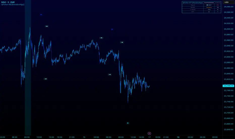
QFisher-R™ [ParadoxAlgo]QFISHER-R™ (Regime-Aware Fisher Transform)
A research/education tool that helps visualize potential momentum exhaustion and probable inflection zones using a quantitative, non-repainting Fisher framework with regime filters and multi-timeframe (MTF) confirmation.
What it does
Converts normalized price movement into a stabilized Fisher domain to highlight potential turning points.
Uses adaptive smoothing, robust (MAD/quantile) thresholds, and optional MTF alignment to contextualize extremes.
Provides a Reversal Probability Score (0–100) to summarize signal confluence (extreme, slope, cross, divergence, regime, and MTF checks).
Key features
Non-repainting logic (bar-close confirmation; security() with no lookahead).
Dynamic exhaustion bands (data-driven thresholds vs fixed ±2).
Adaptive smoothing (efficiency-ratio based).
Optional divergence tags on structurally valid pivots.
MTF confirmation (same logic computed on a higher timeframe).
Compact visuals with subtle plotting to reduce chart clutter.
Inputs (high level)
Source (e.g., HLC3 / Close / HA).
Core lookback, fast/slow range blend, and ER length.
Band sensitivity (robust thresholding).
MTF timeframe(s) and agreement requirement.
Toggle divergence & intrabar previews (default off).
Signals & Alerts
Turn Candidate (Up/Down) when multiple conditions align.
Trade-Grade Turn when score ≥ threshold and MTF agrees.
Divergence Confirmed when structural criteria are met.
Alerts are generated on confirmed bar close by default. Optional “preview” mode is available for experimentation.
How to use
Start on your preferred timeframe; optionally enable an HTF (e.g., 4×) for confirmation.
Look for RPS clusters near the exhaustion bands, slope inflections, and (optionally) divergences.
Combine with your own risk management, liquidity, and trend context.
Paper test first and calibrate thresholds to your instrument and timeframe.
Notes & limitations
This is not a buy/sell signal generator and does not predict future returns.
Readings can remain extreme during strong trends; use HTF context and your own filters.
Parameters are intentionally conservative by default; adjust carefully.
Compliance / Disclaimer
Educational & research tool only. Not financial advice. No recommendation to buy/sell any security or derivative.
Past performance, backtests, or examples (if any) are not indicative of future results.
Trading involves risk; you are responsible for your own decisions and risk management.
Built upon the Fisher Transform concept (Ehlers); all modifications, smoothing, regime logic, scoring, and visualization are original work by Paradox Algo.
ICT + ORB + VIXFix Confluence Signals (Panel)What it is
ICT + ORB + VIXFix Confluence Signals (Panel) is a signal-only Pine v5 indicator that prints clean BUY/SELL arrows when multiple filters align:
ICT structure: BOS / liquidity sweeps + 3-candle FVG with minimum size by ATR
Trend filter: EMA 50 vs EMA 200
ORB filter: opening-range breakout (custom session + minutes)
VIXFix filter: CM_Williams_VIX_Fix–style volatility spike (incl. inverted top)
Status panel: shows which filters are passing and why a signal didn’t fire
No orders are placed; it’s meant to identify trades and trigger alerts.
How signals are built (picky by design)
A BUY arrow paints when all enabled conditions are true:
Trend: EMA50 > EMA200 (or disabled)
ICT: BOS/sweep and bullish FVG (if enabled)
ORB: price breaks above ORB high after the ORB window closes (if enabled)
VIXFix: recent bottom spike within VIX_Lookback bars (if enabled)
A SELL arrow mirrors the above (downtrend, bearish FVG, break below ORB low, recent top spike).
Tip: Leave “Confirm Close Only” on for cleaner signals and fewer repaint-like artifacts.
Inputs (quick reference)
Use Trend (EMA 50/200): require higher-timeframe trend alignment
Use FVG / Use Sweep/BOS: ICT structure filters
SwingLen: pivot left/right length for swings (structure sensitivity)
MinFVG_ATR: minimum FVG size as a fraction of ATR (e.g., 0.20 = 20% ATR)
Session / ORB_Min / Plot_ORB: first N minutes after session open define the range
VIX_LB, VIX_BBLen, VIX_Mult, VIX_Lookback: VIXFix parameters (spike threshold + validity)
Confirm Close Only: only signal at bar close (recommended)
Show Status Panel: compact checklist explaining current filter states
Alerts
Create alerts on this indicator using “Once per bar close” (recommended) and these built-in conditions:
BUY Signal → message: ICT ORB VIXFix BUY
SELL Signal → message: ICT ORB VIXFix SELL
Recommended starting presets
NQ1! / ES1! (US session), intraday 1–5m
Confirm Close Only: ON
Use Trend: ON
Use FVG + Use Sweep/BOS: ON
SwingLen: 3–5
MinFVG_ATR: 0.20–0.30
Session: 0930–1600 (exchange time)
ORB_Min: 10–15
VIXFix: ON, VIX_Lookback 10–20
If you see too few signals, loosen MinFVG_ATR (e.g., 0.10) or temporarily turn off the VIXFix and ORB filters, then re-enable them.
What the panel tells you
Trend (UP/DN): EMA relationship
ICT Long/Short: whether structure/FVG requirements pass for each side
ORB Ready / Long/Short: whether the ORB window is complete and which side broke
VIX Long/Short: recent bottom/top spike validity
Signals: BUY/SELL computed this bar
Why none: quick text reason (trend / ict / orb / vix) if no signal
Notes & attribution
VIXFix is a re-implementation of the CM_Williams_VIX_Fix concept (plus inverted top).
ORB logic uses your chosen session; if your market differs, adjust Session or test on SPY/ES1!/NQ1!.
This is an indicator, not financial advice. Always validate on your instruments/timeframes.
Changelog
v1.0 – Initial release: ICT structure + FVG size by ATR, ORB breakout filter, VIXFix spike filter, trend filter, alerts, and status panel.
Tags
ICT, FVG, ORB, VIX, VIXFix, volatility, structure, BOS, sweep, breakout, EMA, futures, indices, NQ, ES, SPY, day trading, confluence, signals

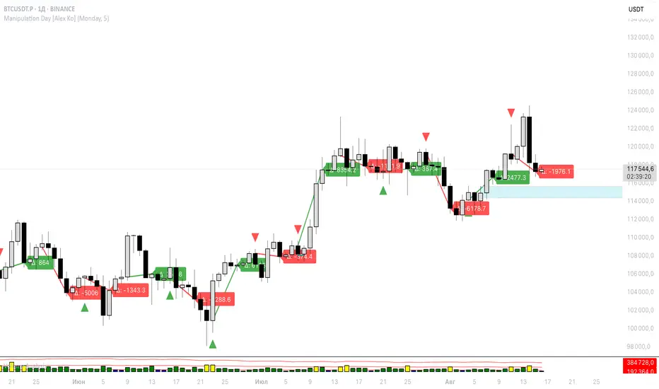
Manipulation Day [Alex Ko]🇺🇸 Description
Indicator “Manipulation Day”
This indicator helps you detect a potential manipulation day (e.g. Monday) and track the price reaction afterward.
📌 Features:
Select any weekday as a manipulation day.
Wait for N candles after it.
If the manipulation day closes higher than it opened — a green triangle appears. If lower — red triangle.
After N days, a line is drawn from the next day's open to the close — green if price increased, red if dropped.
A label shows the delta (Δ) between open and close for that range.
🧠 Useful for spotting potential trap setups or liquidity grabs followed by directional moves.
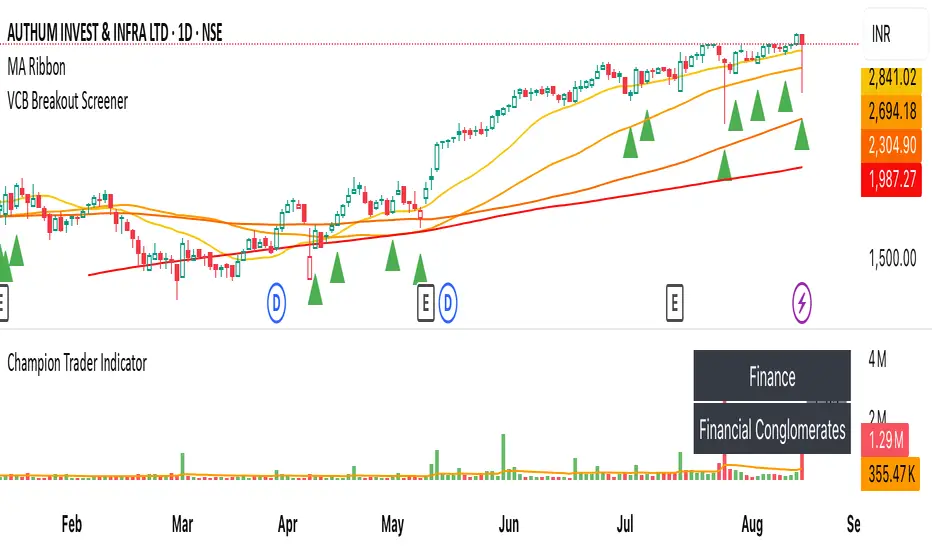
VCB Breakout Screener -PrajaktVCP Breakout Scanner
🔹 How it works
✅ Checks liquidity (vol * price > 100Cr).
✅ Ensures price > SMA50 and SMA100 or SMA200.
✅ ATR filter (short-term > 85% of longer-term).
✅ Price near 40–70% range of the candle.
✅ PGO (close vs SMA/ATR) < 2.5.
✅ RSI(7) < 60.
✅ Plots a green triangle below candles that qualify.
✅ You can set alerts with VCB Breakout condition met!.
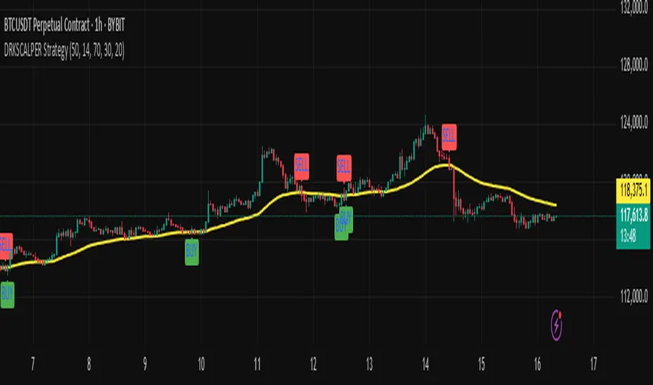
DRKSCALPER Strategy"This indicator is designed to help traders identify market structure shifts, order blocks, and liquidity zones. It is useful for scalping and swing trading, and works on multiple timeframes."
Piman2077: Previous Day Volume Profile levelsPrevious Day Volume Profile Indicator
Description:
Previous Day Volume Profile Indicator plots the previous trading session’s Volume Profile key levels directly on your chart, providing clear reference points for intraday trading. This indicator calculates the Value Area High (VAH), Value Area Low (VAL), and Point of Control (POC) from the prior session and projects them across the current trading day, helping traders identify potential support, resistance, and high-volume zones.
Features:
Calculates previous day VAH, VAL, and POC based on a user-defined session (default 09:30–16:00).
Uses Volume Profile bins for precise distribution calculation.
Fully customizable line colors for VAH, VAL, and POC.
Lines extend across the current session for easy intraday reference.
Works on any timeframe, optimized for 1-minute charts for precision.
Optional toggles to show/hide VAH, VAL, and POC individually.
Inputs:
Session Time: Define the trading session for which the volume profile is calculated.
Profile Bins: Number of price intervals used to divide the session range.
Value Area %: Percentage of volume to include in the value area (default 68%).
Show POC / VAH & VAL: Toggle visibility of each level.
Line Colors: Customize VAH, VAL, and POC colors.
Use Cases:
Identify previous session support and resistance levels for intraday trading.
Gauge areas of high liquidity and potential market reaction zones.
Combine with other indicators or price action strategies for improved entries and exits.
Recommended Timeframe:
Works on all timeframes; best used on 1-minute or 5-minute charts for precise intraday analysis.

Meta-LR ForecastThis indicator builds a forward-looking projection from the current bar by combining twelve time-compressed “mini forecasts.” Each forecast is a linear-regression-based outlook whose contribution is adaptively scaled by trend strength (via ADX) and normalized to each timeframe’s own volatility (via that timeframe’s ATR). The result is a 12-segment polyline that starts at the current price and extends one bar at a time into the future (1× through 12× the chart’s timeframe). Alongside the plotted path, the script computes two summary measures:
* Per-TF Bias% — a directional efficiency × R² score for each micro-forecast, expressed as a percent.
* Meta Bias% — the same score, but applied to the final, accumulated 12-step path. It summarizes how coherent and directional the combined projection is.
This tool is an indicator, not a strategy. It does not place orders. Nothing here is trade advice; it is a visual, quantitative framework to help you assess directional bias and trend context across a ladder of timeframe multiples.
The core engine fits a simple least-squares line on a normalized price series for each small forecast horizon and extrapolates one bar forward. That “trend” forecast is paired with its mirror, an “anti-trend” forecast, constructed around the current normalized price. The model then blends between these two wings according to current trend strength as measured by ADX.
ADX is transformed into a weight (w) in using an adaptive band centered on the rolling mean (μ) with width derived from the standard deviation (σ) of ADX over a configurable lookback. When ADX is deeply below the lower band, the weight approaches -1, favoring anti-trend behavior. Inside the flat band, the weight is near zero, producing neutral behavior. Clearly above the upper band, the weight approaches +1, favoring a trend-following stance. The transitions between these regions are linear so the regime shift is smooth rather than abrupt.
You can shape how quickly the model commits to either wing using two exponents. One exponent controls how aggressively positive weights lean into the trend forecast; the other controls how aggressively negative weights lean into the anti-trend forecast. Raising these exponents makes the response more gradual; lowering them makes the shift more decisive. An optional switch can force full anti-trend behavior when ADX registers a deep-low condition far below the lower tail, if you prefer a categorical stance in very flat markets.
A key design choice is volatility normalization. Every micro-forecast is computed in ATR units of its own timeframe. The script fetches that timeframe’s ATR inside each security call and converts normalized outputs back to price with that exact ATR. This avoids scaling higher-timeframe effects by the chart ATR or by square-root time approximations. Using “ATR-true” for each timeframe keeps the cross-timeframe accumulation consistent and dimensionally correct.
Bias% is defined as directional efficiency multiplied by R², expressed as a percent. Directional efficiency captures how much net progress occurred relative to the total path length; R² captures how well the path aligns with a straight line. If price meanders without net progress, efficiency drops; if the variation is well-explained by a line, R² rises. Multiplying the two penalizes choppy, low-signal paths and rewards sustained, coherent motion.
The forward path is built by converting each per-timeframe Bias% into a small ATR-sized delta, then cumulatively adding those deltas to form a 12-step projection. This produces a polyline anchored at the current close and stepping forward one bar per timeframe multiple. Segment color flips by slope, allowing a quick read of the path’s direction and inflection.
Inputs you can tune include:
* Max Regression Length. Upper bound for each micro-forecast’s regression window. Larger values smooth the trend estimate at the cost of responsiveness; smaller values react faster but can add noise.
* Price Source. The price series analyzed (for example, close or typical price).
* ADX Length. Period used for the DMI/ADX calculation.
* ATR Length (normalization). Window used for ATR; this is applied per timeframe inside each security call.
* Band Lookback (for μ, σ). Lookback used to compute the adaptive ADX band statistics. Larger values stabilize the band; smaller values react more quickly.
* Flat half-width (σ). Width of the neutral band on both sides of μ. Wider flats spend more time neutral; narrower flats switch regimes more readily.
* Tail width beyond flat (σ). Distance from the flat band edge to the extreme trend/anti-trend zone. Larger tails create a longer ramp; smaller tails reach extremes sooner.
* Polyline Width. Visual thickness of the plotted segments.
* Negative Wing Aggression (anti-trend). Exponent shaping for negative weights; higher values soften the tilt into mean reversion.
* Positive Wing Aggression (trend). Exponent shaping for positive weights; lower values make trend commitment stronger and sooner.
* Force FULL Anti-Trend at Deep-Low ADX. Optional hard switch for extremely low ADX conditions.
On the chart you will see:
* A 12-segment forward polyline starting from the current close to bar\_index + 1 … +12, with green segments for up-steps and red for down-steps.
* A small label at the latest bar showing Meta Bias% when available, or “n/a” when insufficient data exists.
Interpreting the readouts:
* Trend-following contexts are characterized by ADX above the adaptive upper band, pushing w toward +1. The blended forecast leans toward the regression extrapolation. A strongly positive Meta Bias% in this environment suggests directional alignment across the ladder of timeframes.
* Mean-reversion contexts occur when ADX is well below the lower tail, pushing w toward -1 (or forcing anti-trend if enabled). After a sharp advance, a negative Meta Bias% may indicate the model projects pullback tendencies.
* Neutral contexts occur when ADX sits inside the flat band; w is near zero, the blended forecast remains close to current price, and Meta Bias% tends to hover near zero.
These are analytical cues, not rules. Always corroborate with your broader process, including market structure, time-of-day behavior, liquidity conditions, and risk limits.
Practical usage patterns include:
* Momentum confirmation. Combine a rising Meta Bias% with higher-timeframe structure (such as higher highs and higher lows) to validate continuation setups. Treat the 12th step’s distance as a coarse sense of potential room rather than as a target.
* Fade filtering. If you prefer fading extremes, require ADX to be near or below the lower ramp before acting on counter-moves, and avoid fades when ADX is decisively above the upper band.
* Position planning. Because per-step deltas are ATR-scaled, the path’s vertical extent can be mentally mapped to typical noise for the instrument, informing stop distance choices. The script itself does not compute orders or size.
* Multi-timeframe alignment. Each step corresponds to a clean multiple of your chart timeframe, so the polyline visualizes how successively larger windows bias price, all referenced to the current bar.
House-rules and repainting disclosures:
* Indicator, not strategy. The script does not execute, manage, or suggest orders. It displays computed paths and bias scores for analysis only.
* No performance claims. Past behavior of any measure, including Meta Bias%, does not guarantee future results. There are no assurances of profitability.
* Higher-timeframe updates. Values obtained via security for higher-timeframe series can update intrabar until the higher-timeframe bar closes. The forward path and Meta Bias% may change during formation of a higher-timeframe candle. If you need confirmed higher-timeframe inputs, consider reading the prior higher-timeframe value or acting only after the higher-timeframe close.
* Data sufficiency. The model requires enough history to compute ATR, ADX statistics, and regression windows. On very young charts or illiquid symbols, parts of the readout can be unavailable until sufficient data accumulates.
* Volatility regimes. ATR normalization helps compare across timeframes, but unusual volatility regimes can make the path look deceptively flat or exaggerated. Judge the vertical scale relative to your instrument’s typical ATR.
Tuning tips:
* Stability versus responsiveness. Increase Max Regression Length to steady the micro-forecasts but accept slower response. If you lower it, consider slightly increasing Band Lookback so regime boundaries are not too jumpy.
* Regime bands. Widen the flat half-width to spend more time neutral, which can reduce over-trading tendencies in chop. Shrink the tail width if you want the model to commit to extremes sooner, at the cost of more false swings.
* Wing shaping. If anti-trend behavior feels too abrupt at low ADX, raise the negative wing exponent. If you want trend bias to kick in more decisively at high ADX, lower the positive wing exponent. Small changes have large effects.
* Forced anti-trend. Enable the deep-low option only if you explicitly want a categorical “markets are flat, fade moves” policy. Many users prefer leaving it off to keep regime decisions continuous.
Troubleshooting:
* Nothing plots or the label shows “n/a.” Ensure the chart has enough history for the ADX band statistics, ATR, and the regression windows. Exotic or illiquid symbols with missing data may starve the higher-timeframe computations. Try a more liquid market or a higher timeframe.
* Path flickers or shifts during the bar. This is expected when any higher-timeframe input is still forming. Wait for the higher-timeframe close for fully confirmed behavior, or modify the code to read prior values from the higher timeframe.
* Polyline looks too flat or too steep. Check the chart’s vertical scale and recent ATR regime. Adjust Max Regression Length, the wing exponents, or the band widths to suit the instrument.
Integration ideas for manual workflows:
* Confluence checklist. Use Meta Bias% as one of several independent checks, alongside structure, session context, and event risk. Act only when multiple cues align.
* Stop and target thinking. Because deltas are ATR-scaled at each timeframe, benchmark your proposed stops and targets against the forward steps’ magnitude. Stops that are much tighter than the prevailing ATR often sit inside normal noise.
* Session context. Consider session hours and microstructure. The same ADX value can imply different tradeability in different sessions, particularly in index futures and FX.
This indicator deliberately avoids:
* Fixed thresholds for buy or sell decisions. Markets vary and fixed numbers invite overfitting. Decide what constitutes “high enough” Meta Bias% for your market and timeframe.
* Automatic risk sizing. Proper sizing depends on account parameters, instrument specifications, and personal risk tolerance. Keep that decision in your risk plan, not in a visual bias tool.
* Claims of edge. These measures summarize path geometry and trend context; they do not ensure a tradable edge on their own.
Summary of how to think about the output:
* The script builds a 12-step forward path by stacking linear-regression micro-forecasts across increasing multiples of the chart timeframe.
* Each micro-forecast is blended between trend and anti-trend using an adaptive ADX band with separate aggression controls for positive and negative regimes.
* All computations are done in ATR-true units for each timeframe before reconversion to price, ensuring dimensional consistency when accumulating steps.
* Bias% (per-timeframe and Meta) condenses directional efficiency and trend fidelity into a compact score.
* The output is designed to serve as an analytical overlay that helps assess whether conditions look trend-friendly, fade-friendly, or neutral, while acknowledging higher-timeframe update behavior and avoiding prescriptive trade rules.
Use this tool as one component within a disciplined process that includes independent confirmation, event awareness, and robust risk management.

Indicador Millo SMA20-SMA200-AO-RSI M1This indicator is designed for scalping in 1-minute timeframes on crypto pairs, combining trend direction, momentum, and oscillator confirmation.
Logic:
Trend Filter:
Only BUY signals when price is above the SMA200.
Only SELL signals when price is below the SMA200.
Entry Trigger:
BUY: Price crosses above the SMA20.
SELL: Price crosses below the SMA20.
Confirmation Window:
After the price cross, the Awesome Oscillator (AO) must cross the zero line in the same direction within a maximum of N bars (configurable, default = 4).
RSI must be > 50 for BUY and < 50 for SELL at the moment AO confirms.
Cooldown:
A cooldown period (configurable, default = 10 bars) prevents multiple signals of the same type in a short time, reducing noise in sideways markets.
Features:
Works on any crypto pair and can be used in other markets.
Adjustable confirmation window, RSI threshold, and cooldown.
Alerts ready for BUY and SELL conditions.
Can be converted into a strategy for backtesting with TP/SL.
Suggested Use:
Pair: BTC/USDT M1 or similar high-liquidity asset.
Combine with manual support/resistance or higher timeframe trend analysis.
Recommended to confirm entries visually and with additional confluence before trading live.

MistaB SMC Navigation ToolkitMistaB SMC Navigation Toolkit
A complete Smart Money Concepts (SMC) toolkit designed for precision navigation of market structure, order flow, and premium/discount trading zones. Perfect for traders following ICT-style concepts and multi-timeframe confluence.
Features
✅ Order Blocks (OBs)
• Automatic bullish & bearish OB detection
• Optional displacement & high-volume filters
• Midline display for quick equilibrium view
• Auto-expiry and broken OB cleanup
✅ Fair Value Gaps (FVGs)
• Bullish & bearish gap detection
• HTF bias filtering for higher accuracy
• Compact boxes with labels
• Automatic removal when filled
✅ Market Structure (BoS / CHoCH)
• Fractal-based swing detection
• Break of Structure & Change of Character labeling
• Dynamic HTF bias dimming
✅ Premium / Discount Zones
• Auto-calculated mid-level
• Highlighted zones for optimal trade placement
✅ Higher Timeframe (HTF) Confirmation
• Configurable confirmation timeframe
• On-chart HTF status label (Bullish / Bearish / Not Required)
✅ Automatic Cleanup System
• Fast or delayed cleanup for expired/broken zones
• Dimmed colors for invalidated levels
How to Use
Set your preferred HTF in the settings.
Look for OB/FVGs aligned with HTF bias.
Enter in discount zones for longs or premium zones for shorts.
Confirm with BoS / CHoCH signals before entry.
Manage trades towards opposing liquidity zones or HTF levels.
Disclaimer
This indicator is for educational purposes only. It does not provide financial advice or guarantee future results. Always practice proper risk management and test thoroughly before live trading.

Kootch EMA MapKootch EMA overlays the 200 EMA from M1, M5, M15, M30, H1, H4, and D1 on any chart so you always see where higher and lower-timeframe trend gravity actually is. It also builds an optional Fib channel between the most extreme MTF 200 EMAs (min/max), giving you clean intrachannel targets and confluence zones.
What it does
• Plots seven 200 EMAs (M1 → D1) simultaneously via MTF pulls
• Color/weight hierarchy: thicker lines = higher timeframe (clear priority)
• Right-edge TF tags (M1, M5, … D1) so you know exactly what you’re looking at
• Optional Fib levels between min/max MTF 200 EMAs (0 → 1 band) for entries, adds, and take-profit scaling
Why traders use it
• Immediate read on trend alignment vs. chop across timeframes
• Mean-reversion & continuation cues when price stretches from/returns to key EMAs
• Level stacking: use M30/H1/H4/D1 as bias, trade entries around lower-TF reactions
Inputs
• EMA Length (default 200)
• Label offset (push tags off the last bar)
• Show Fib channel toggle + color control
How I use it
• Bias from D1/H4/H1; execution from M5/M15.
• Fade or follow at Fib 0.382 / 0.618 inside the EMA envelope; scale out near Fib 1.0 into HTF EMAs.
• Skip trades when EMAs are braided and distances are compressed.
Notes
• Works on any symbol/timeframe; all TF EMAs are requested explicitly.
• This is a map, not a crystal ball: combine with your playbook (structure breaks, FVGs, liquidity, volume).

ATR: Body % + Ranges and AnomaliesATR: Body % + Ranges and Anomalies
This indicator provides a dual analysis of price bars to help you better understand market dynamics and volatility. It combines two powerful concepts into one tool: a candle body percentage and a range analysis with an anomaly-excluding average.
Key Features:
1. Candle Body Percentage
This feature plots the size of the candle's body as a percentage of its total high-low range.
A high percentage (e.g., above the 50% gray line) indicates strong, directional movement. The more solid the body is relative to its wicks, the more conviction is behind that move.
The 100% red line marks "Marubozu" candles—bars with no wicks, showing absolute control by buyers or sellers.
2. Range Analysis with Anomalies
This is a unique part of the indicator that helps you identify and understand normal vs. abnormal volatility.
Custom SMA: It calculates an average range of the last N bars, but it smartly excludes "anomalous" bars (spikes or unusually small ranges) from the calculation. This gives you a more reliable baseline for normal volatility.
Anomaly Detection: Bars are colored differently based on their range:
Blue: Small anomalies (range less than 0.5 * ATR). These often occur during periods of low liquidity or indecision.
Red: Large anomalies (range greater than 1.8 * ATR). These can signal a sudden burst of volatility, breakout events, or capitulation.
ATR Range % Label: The label on the chart shows the current bar's range as a percentage of the custom SMA. This tells you how much larger or smaller the current bar's range is compared to a clean average.
How to Use:
Spotting Trends: Use the Body % to confirm the strength of a trend. A series of bars with high body percentages can indicate a strong, healthy trend.
Identifying Volatility: Use the Range Analysis to find areas of interest. A large red anomaly bar could signal a significant event, while a series of blue anomalies might suggest the market is in a tight consolidation before a breakout.
Contextual Analysis: The combination of these tools can provide powerful context. For example, a bar with a high Body % and a red anomaly color suggests a strong, volatile move that could be a turning point or the start of a major trend.
Experiment with the input settings to fine-tune the ATR and SMA periods for different timeframes and assets.

EAOBS by MIGVersion 1
1. Strategy Overview Objective: Capitalize on breakout movements in Ethereum (ETH) price after the Asian open pre-market session (7:00 PM–7:59 PM EST) by identifying high and low prices during the session and trading breakouts above the high or below the low.
Timeframe: Any (script is timeframe-agnostic, but align with session timing).
Session: Pre-market session (7:00 PM–7:59 PM EST, adjustable for other time zones, e.g., 12:00 AM–12:59 AM GMT).
Risk-Reward Ratios (R:R): Targets range from 1.2:1 to 5.2:1, with a fixed stop loss.
Instrument: Ethereum (ETH/USD or ETH-based pairs).
2. Market Setup Session Monitoring: Monitor ETH price action during the pre-market session (7:00 PM–7:59 PM EST), which aligns with the Asian market open (e.g., 9:00 AM–9:59 AM JST).
The script tracks the highest high and lowest low during this session.
Breakout Triggers: Buy Signal: Price breaks above the session’s high after the session ends (7:59 PM EST).
Sell Signal: Price breaks below the session’s low after the session ends.
Visualization: The session is highlighted on the chart with a white background.
Horizontal lines are drawn at the session’s high and low, extended for 30 bars, along with take-profit (TP) and stop-loss (SL) levels.
3. Entry Rules Long (Buy) Entry: Enter a long position when the price breaks above the session’s high price after 7:59 PM EST.
Entry price: Just above the session high (e.g., add a small buffer, like 0.1–0.5%, to avoid false breakouts, depending on volatility).
Short (Sell) Entry: Enter a short position when the price breaks below the session’s low price after 7:59 PM EST.
Entry price: Just below the session low (e.g., subtract a small buffer, like 0.1–0.5%).
Confirmation: Use a candlestick close above/below the breakout level to confirm the entry.
Optionally, add volume confirmation or a momentum indicator (e.g., RSI or MACD) to filter out weak breakouts.
Position Size: Calculate position size based on risk tolerance (e.g., 1–2% of account per trade).
Risk is determined by the stop-loss distance (10 points, as defined in the script).
4. Exit Rules Take-Profit Levels (in points, based on script inputs):TP1: 12 points (1.2:1 R:R).
TP2: 22 points (2.2:1 R:R).
TP3: 32 points (3.2:1 R:R).
TP4: 42 points (4.2:1 R:R).
TP5: 52 points (5.2:1 R:R).
Example for Long: If session high is 3000, TP levels are 3012, 3022, 3032, 3042, 3052.
Example for Short: If session low is 2950, TP levels are 2938, 2928, 2918, 2908, 2898.
Strategy: Scale out of the position (e.g., close 20% at TP1, 20% at TP2, etc.) or take full profit at a preferred TP level based on market conditions.
Stop-Loss: Fixed at 10 points from the entry.
Long SL: Session high - 10 points (e.g., entry at 3000, SL at 2990).
Short SL: Session low + 10 points (e.g., entry at 2950, SL at 2960).
Trailing Stop (Optional):After reaching TP2 or TP3, consider trailing the stop to lock in profits (e.g., trail by 10–15 points below the current price).
5. Risk Management per Trade: Limit risk to 1–2% of your trading account per trade.
Calculate position size: Account Size × Risk % ÷ (Stop-Loss Distance × ETH Price per Point).
Example: $10,000 account, 1% risk = $100. If SL = 10 points and 1 point = $1, position size = $100 ÷ 10 = 0.1 ETH.
Daily Risk Limit: Cap daily losses at 3–5% of the account to avoid overtrading.
Maximum Exposure: Avoid taking both long and short positions simultaneously unless using separate accounts or strategies.
Volatility Consideration: Adjust position size during high-volatility periods (e.g., major news events like Ethereum upgrades or macroeconomic announcements).
6. Trade Management Monitoring :Watch for breakouts after 7:59 PM EST.
Monitor price action near TP and SL levels using alerts or manual checks.
Trade Duration: Breakout lines extend for 30 bars (script parameter). Close trades if no TP or SL is hit within this period, or reassess based on market conditions.
Adjustments: If the market shows strong momentum, consider holding beyond TP5 with a trailing stop.
If the breakout fails (e.g., price reverses before TP1), exit early to minimize losses.
7. Additional Considerations Market Conditions: The 7:00 PM–7:59 PM EST session aligns with the Asian market open (e.g., Tokyo Stock Exchange open at 9:00 AM JST), which may introduce higher volatility due to Asian trading activity.
Avoid trading during low-liquidity periods or extreme volatility (e.g., major crypto news).
Check for upcoming events (e.g., Ethereum network upgrades, ETF decisions) that could impact price.
Backtesting: Test the strategy on historical ETH data using the session high/low breakouts for the 7:00 PM–7:59 PM EST window to validate performance.
Adjust TP/SL levels based on backtest results if needed.
Broker and Fees: Use a low-fee crypto exchange (e.g., Binance, Kraken, Coinbase Pro) to maximize R:R.
Account for trading fees and slippage in your position sizing.
Time zone Adjustment: Adjust session time input for your time zone (e.g., "0000-0059" for GMT).
Ensure your trading platform’s clock aligns with the script’s time zone (default: America/New_York).
8. Example Trade Scenario: Session (7:00 PM–7:59 PM EST) records a high of 3050 and a low of 3000.
Long Trade: Entry: Price breaks above 3050 (e.g., enter at 3051).
TP Levels: 3063 (TP1), 3073 (TP2), 3083 (TP3), 3093 (TP4), 3103 (TP5).
SL: 3040 (3050 - 10).
Position Size: For a $10,000 account, 1% risk = $100. SL = 11 points ($11). Size = $100 ÷ 11 = ~0.09 ETH.
Short Trade: Entry: Price breaks below 3000 (e.g., enter at 2999).
TP Levels: 2987 (TP1), 2977 (TP2), 2967 (TP3), 2957 (TP4), 2947 (TP5).
SL: 3010 (3000 + 10).
Position Size: Same as above, ~0.09 ETH.
Execution: Set alerts for breakouts, enter with limit orders, and monitor TPs/SL.
9. Tools and Setup Platform: Use TradingView to implement the Pine Script and visualize breakout levels.
Alerts: Set price alerts for breakouts above the session high or below the session low after 7:59 PM EST.
Set alerts for TP and SL levels.
Chart Settings: Use a 1-minute or 5-minute chart for precise session tracking.
Overlay the script to see high/low lines, TP levels, and SL levels.
Optional Indicators: Add RSI (e.g., avoid overbought/oversold breakouts) or volume to confirm breakouts.
10. Risk Warnings Crypto Volatility: ETH is highly volatile; unexpected news can cause rapid price swings.
False Breakouts: Breakouts may fail, especially in low-volume sessions. Use confirmation signals.
Leverage: Avoid high leverage (e.g., >5x) to prevent liquidation during volatile moves.
Session Accuracy: Ensure correct session timing for your time zone to avoid misaligned entries.
11. Performance Tracking Journaling :Record each trade’s entry, exit, R:R, and outcome.
Note market conditions (e.g., trending, ranging, news-driven).
Review: Weekly: Assess win rate, average R:R, and adherence to the plan.
Monthly: Adjust TP/SL or session timing based on performance.