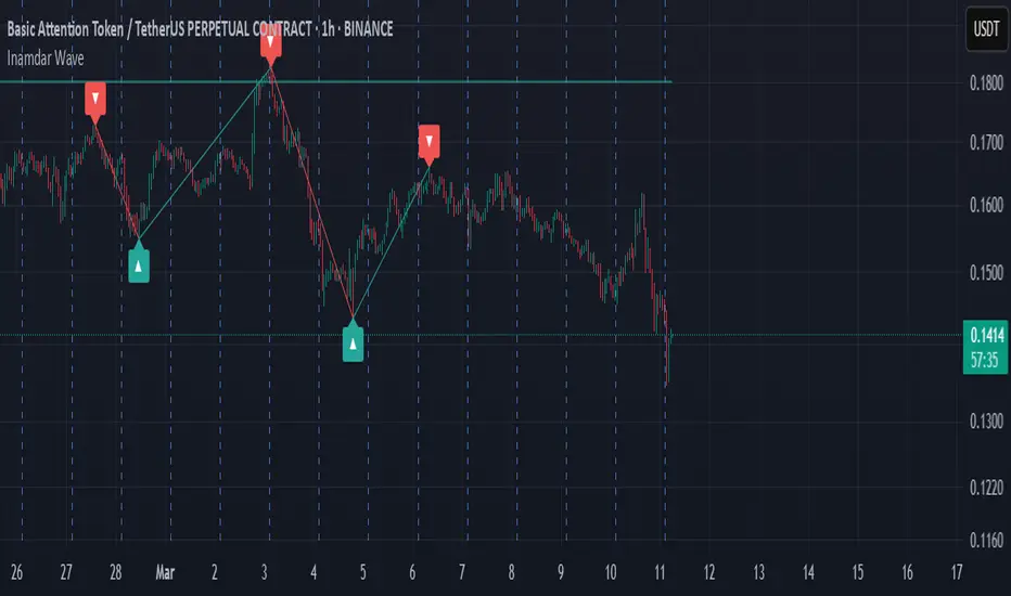
Position Size Calculator for ContractDescription:
Position Size Calculator is a versatile Pine Script tool designed to help traders manage their risk and position sizing effectively. This script calculates essential trading metrics and visualizes them directly on your chart, helping you make informed trading decisions.
Features:
- Account Size & Risk Management:
- Account Size: Input your total account balance to calculate position sizes.
- Maximum Risk: Define how much of your account you are willing to risk per trade in dollars.
- Pip Value: Set the value of a single pip for one contract, which is crucial for calculating risk
and position size.
Trade Setup Visualization:
- Entry Price: Specify the price at which you plan to enter the trade.
- Stop Loss: Define your stop loss level to manage your risk.
- Take Profit: Set your target profit level for the trade.
- Visualize the Entry, Stop Loss, and Take Profit levels on your chart with customizable line
colors and text sizes.
- View the distance in pips between the Entry, Stop Loss, and Take Profit levels.
Position Size Calculation:
- Calculates the number of contracts to open based on your risk tolerance and the pip value.
- Displays the maximum number of contracts you can open given your risk parameters.
Customizable Table Display:
- Table Position: Choose the position of the summary table on the chart (Top-Left, Top-Right,
Bottom-Left, Bottom-Right, etc.).
- Table Text Size: Adjust the text size for the summary table.
- Table Background Color: Set the background color for the summary table.
- Table Border Color: Customize the border color of the summary table.
How to Use:
1- Input your Account Size: Enter your current account balance.
2- Set Maximum Risk and Pip Value: Define how much you're willing to risk per trade and the
pip value for your contract.
3- Define Trade Levels: Input your desired Entry Price, Stop Loss, and Take Profit levels.
4- Customize Visuals: Adjust the line styles and table settings to fit your preferences.
5- View Calculations: The script will display the distance in pips and the calculated position
size directly on your chart.
Example Usage:
Example to calculate the value of 1 pips with 1 contract:
Inputs:
Account Size: Your total trading account balance.
Maximum Risk: Risk amount per trade in dollars.
Pip Value: Value of one pip for a single contract.
Entry Price: The price at which you plan to enter the trade.
Stop Loss: The level at which you will exit the trade to cut losses.
Take Profit: The target price to lock in profits.
Line Text Size: Size of the text for the Entry, Stop Loss, and Take Profit lines.
Line Extend: Option to extend the lines for visual clarity.
Table Position: Position of the summary table on the chart.
Table Text Size: Size of the text in the summary table.
Table Background Color: Background color of the summary table.
Table Border Color: Border color of the summary table.
Visuals:
Entry Price, Stop Loss, and Take Profit levels are clearly marked on the chart.
Summary Table with important trade metrics displayed.
Cari dalam skrip untuk "profit"
MAC Investor V3.0 [VK]This indicator combines multiple functionalities to assist traders in making informed decisions. It primarily uses Heikin Ashi candles, Moving Averages, and a Price Action Channel (PAC) to provide signals for entering and exiting trades. Here's a detailed breakdown:
Inputs
MAC Length: Sets the length for the PAC calculation.
Use Heikin Ashi Candles: Option to use Heikin Ashi candles for calculations.
Show Coloured Bars around MAC: Option to color bars based on their relation to the PAC.
Show Long/Short Signals: Options to display long and short signals.
Show MAs? : Option to show moving averages on the chart.
Show MAs Trend at the Bottom?: Option to show trend signals at the bottom of the chart.
MA Lengths: Length settings for three different moving averages.
Change MA Color Based on Direction?: Option to change the color of moving averages based on trend direction.
MA Higher TimeFrame: Allows setting a higher timeframe for moving averages.
Show SL-TP Lines: Option to display Stop Loss and Take Profit lines.
SL/TP Percentages: Set the percentages for Stop Loss and three levels of Take Profit.
Calculations and Features
Heikin Ashi Candles: Calculations are based on Heikin Ashi candle data if selected.
Price Action Channel (PAC): Uses Exponential Moving Averages (EMA) of the high, low, and close to create a channel.
Bar Coloring: Colors the bars based on their position relative to the PAC.
Long and Short Signals: Uses crossovers of the close price and PAC upper/lower bands to generate signals.
Moving Averages (MA): Plots three moving averages and colors them based on their trend direction.
Overall Trend Indicators: Uses triangles at the bottom of the chart to show the overall trend of the MAs.
Stop Loss and Take Profit Levels: Calculates and plots these levels based on user-defined percentages from the entry price.
Alerts: Provides alerts for long and short signals.
Use Cases and How to Use
Identifying Trends: The PAC helps to identify the trend direction. If the closing price is above the PAC upper band, it suggests an uptrend; if below the lower band, it suggests a downtrend.
Entering Trades: Use the long and short signals to enter trades. A long signal is generated when the closing price crosses above the PAC upper band, and a short signal is generated when it crosses below the PAC lower band.
Exit Strategies: Utilize the Stop Loss (SL) and Take Profit (TP) levels to manage risk and lock in profits. These levels are automatically calculated based on the entry price and user-defined percentages.
Trend Confirmation with MAs: The moving averages provide additional confirmation of the trend. When all three MAs are trending in the same direction (e.g., all green for an uptrend), it adds confidence to the trade signal.
Overall Trend Indicators: The triangles at the bottom of the chart show the overall trend direction of the MAs:
Green Triangle: All three MAs are trending upwards, indicating a strong uptrend.
Red Triangle: All three MAs are trending downwards, indicating a strong downtrend.
Yellow Triangle: Mixed signals from the MAs, indicating no clear trend.
Bar Coloring for Quick Analysis: The colored bars give a quick visual cue about the market condition, aiding in faster decision-making.
Alerts: Set up alerts to get notified when a long or short signal is generated, allowing you to act promptly without constantly monitoring the chart.
Maximizing Profit
To maximize profit with this indicator:
Follow the Signals: Use the long and short signals to time your entries. Ensure you follow the trend indicated by the PAC and MAs.
Risk Management: Always set your Stop Loss and Take Profit levels to manage risk. This will help you cut losses early and secure profits.
Confirm with MAs: Look for confirmation from the moving averages. When all MAs align with the signal, it indicates a stronger trend.
Overall Trend Indicators: Pay attention to the triangles at the bottom for overall trend confirmation. Only enter trades when the overall trend is in your favor.
Heikin Ashi for Smoothing: Use Heikin Ashi candles for smoother trends and fewer false signals.
Backtesting: Test the indicator on historical data to understand its performance and adjust settings as necessary.
Adapt to Market Conditions: Adjust the lengths of PAC and MAs based on the market's volatility and timeframe you are trading on.
How to Use the Indicator
Add to Chart: Add the indicator to your TradingView chart.
Configure Settings: Customize the input settings to fit your trading strategy and timeframe.
Monitor Signals: Watch for long and short signals and observe the trend direction with the PAC and MAs.
Check Overall Trend: Look at the triangles at the bottom of the chart to see the overall trend direction of the MAs.
Set Alerts: Configure alerts to get notified of new signals.
Manage Trades: Use the SL and TP levels to manage your trades effectively.
Grid TraderGrid Trader Indicator ( GTx ):
Overview
The Grid Trader Indicator is a tool that helps traders visualize key levels within a specified trading range. The indicator plots accumulation and distribution levels, an entry level, an exit level, and a midpoint. This guide will help you understand how to use the indicator and its features for effective grid trading.
Basics of Trading Range, Grid Buy, and Grid Sell
Trading Range
A trading range is the horizontal price movement between a defined upper ( resistance ) and lower ( support ) level over a period of time. When a security trades within a range, it repeatedly moves between these two levels without trending upwards or downwards significantly. Traders often use the trading range to identify potential buy and sell points:
Upper Level (Resistance): This is the price level at which selling pressure overcomes buying pressure, preventing the price from rising further.
Lower Level (Support): This is the price level at which buying pressure overcomes selling pressure, preventing the price from falling further.
Grid Trading Strategy
Grid trading is a type of trading strategy that involves placing buy and sell orders at predefined intervals around a set price. It aims to profit from the natural market volatility by buying low and selling high in a range-bound market. The strategy divides the trading range into several grid levels where orders are placed.
Grid Buy
Grid buy orders are placed at intervals below the current price . When the price drops to these levels, buy orders are triggered . This strategy ensures that the trader buys more as the price falls, potentially lowering the average purchase price .
Grid Sell
Grid sell orders are placed at intervals above the current price . When the price rises to these levels, sell orders are triggered . This ensures that the trader sells portions of their holdings as the price increases, potentially securing profits at higher levels .
Key Points of Grid Trading
Grid Size : The interval between each buy and sell order. This can be constant (e.g., $2 intervals) or variable based on certain conditions.
Accumulation Range : The lower part of the trading range where buy orders are placed.
Distribution Range : The upper part of the trading range where sell orders are placed.
Midpoint : The average price of the entry and exit levels, often used as a reference point for balance.
As the price moves up and down within this range, your buy orders will be triggered as the price drops and your sell orders will be triggered as the price rises. This allows you to accumulate more of the asset at lower prices and sell portions at higher prices, profiting from the price oscillations within the defined range. Grid trading can be particularly effective in a sideways market where there is no clear long-term trend. However, it requires careful monitoring and adjustment of grid levels based on market conditions to minimize risks and maximize returns .
Configuring the Indicator :
Once the indicator is added, you will see a settings icon next to it. Click on it to open the settings menu.
Adjust the Upper Level , Lower Level , Entry Level , and Exit Level to match your trading strategy and market conditions.
Set the Levels Visibility to control how many bars back the levels will be plotted.
Interpreting the Levels :
Accumulation Levels : These are plotted below the entry level and are potential buy zones. They are labeled as Accumulation Level 1, 2, and 3.
Distribution Levels : These are plotted above the exit level and are potential sell zones. They are labeled as Distribution Level 1, 2, and 3.
Upper Level : Marked in fuchsia, indicating the top boundary of the trading range.
Exit Level : Marked in yellow, indicating the level at which you plan to exit trades.
Midpoint : Marked in white, indicating the average of the entry and exit levels.
Entry Level : Marked in yellow, indicating the level at which you plan to enter trades.
Lower Level : Marked in aqua, indicating the bottom boundary of the trading range.
By visualizing key levels, you can make informed decisions on where to place buy and sell orders, potentially maximizing your trading profits through systematic grid trading.
Wolf DCA CalculatorThe Wolf DCA Calculator is a powerful and flexible indicator tailored for traders employing the Dollar Cost Averaging (DCA) strategy. This tool is invaluable for planning and visualizing multiple entry points for both long and short positions. It also provides a comprehensive analysis of potential profit and loss based on user-defined parameters, including leverage.
Features
Entry Price: Define the initial entry price for your trade.
Total Lot Size: Specify the total number of lots you intend to trade.
Percentage Difference: Set the fixed percentage difference between each DCA point.
Long Position: Toggle to switch between long and short positions.
Stop Loss Price: Set the price level at which you plan to exit the trade to minimize losses.
Take Profit Price: Set the price level at which you plan to exit the trade to secure profits.
Leverage: Apply leverage to your trade, which multiplies the potential profit and loss.
Number of DCA Points: Specify the number of DCA points to strategically plan your entries.
How to Use
1. Add the Indicator to Your Chart:
Search for "Wolf DCA Calculator" in the TradingView public library and add it to your chart.
2. Configure Inputs:
Entry Price: Set your initial trade entry price.
Total Lot Size: Enter the total number of lots you plan to trade.
Percentage Difference: Adjust this to set the interval between each DCA point.
Long Position: Use this toggle to choose between a long or short position.
Stop Loss Price: Input the price level at which you plan to exit the trade to minimize losses.
Take Profit Price: Input the price level at which you plan to exit the trade to secure profits.
Leverage: Set the leverage you are using for the trade.
Number of DCA Points: Specify the number of DCA points to plan your entries.
3. Analyze the Chart:
The indicator plots the DCA points on the chart using a stepline style for clear visualization.
It calculates the average entry point and displays the potential profit and loss based on the specified leverage.
Labels are added for each DCA point, showing the entry price and the lots allocated.
Horizontal lines mark the Stop Loss and Take Profit levels, with corresponding labels showing potential loss and profit.
Benefits
Visual Planning: Easily visualize multiple entry points and understand how they affect your average entry price.
Risk Management: Clearly see your Stop Loss and Take Profit levels and their impact on your trade.
Customizable: Adapt the indicator to your specific strategy with a wide range of customizable parameters.
Dividend-to-ROE RatioDividend-to-ROE Ratio Indicator
The Dividend-to-ROE Ratio indicator offers valuable insights into a company's dividend distribution relative to its profitability, specifically comparing the Dividend Payout Ratio (proportion of earnings as dividends) to the Return on Equity (ROE), a measure of profitability from shareholder equity.
Interpretation:
1. Higher Ratio: A higher Dividend-to-ROE Ratio suggests a stable dividend policy, where a significant portion of earnings is returned to shareholders. This can indicate consistent dividend payments, often appealing to income-seeking investors.
2. Lower Ratio: Conversely, a lower ratio implies that the company retains more earnings for growth, potentially signaling a focus on reinvestment for future expansion rather than immediate dividend payouts.
3. Excessively High Ratio: An exceptionally high ratio may raise concerns. While it could reflect a generous dividend policy, excessively high ratios might indicate that a company is distributing more earnings than it can sustainably afford. This could potentially hinder the company's ability to reinvest in its operations, research, or navigate economic downturns effectively.
Utility and Applications:
The Dividend-to-ROE Ratio can be particularly useful in the following scenarios:
1. Income-Oriented Investors: For investors seeking consistent dividend income, a higher ratio signifies a company's commitment to distributing profits to shareholders, potentially aligning with income-oriented investment strategies.
2. Financial Health Assessment: Analysts and stakeholders can use this ratio to gauge a company's financial health and dividend sustainability. It provides insights into management's capital allocation decisions and strategic focus.
3. Comparative Analysis: When comparing companies within the same industry, this ratio helps in benchmarking dividend policies and identifying outliers with unusually high or low ratios.
Considerations:
1. Contextual Analysis: Interpretation should be contextualized within industry standards and the company's financial history. Comparing the ratio with peers in the same sector can provide meaningful insights.
2. Financial Health: It's crucial to evaluate this indicator alongside other financial metrics (like cash flow, debt levels, and profit margins) to grasp the company's overall financial health and sustainability of its dividend policy.
Disclaimer: This indicator is for informational purposes only and does not constitute financial advice. Investors should conduct thorough research and consult with financial professionals before making investment decisions based on this ratio.
PUELL - PUELL Top and Bottom Indicator for BTC [Logue]Puell Multiple Indicator (PUELL) - The Puell multiple is the ratio between the daily coin issuance in USD and its 365-day moving average. This multiple helps to measure miner profitability. The PUELL indicator smooths the Puell multiple using a 14-day simple moving average. When the PUELL goes to high values relative to historical values, it indicates the profitability of the miners is high and a top may be near. When the PUELL is low relative to historical values, it indicates the profitability of the minors is low and a bottom may be near. The default trigger values are PUELL values above 3.0 for a "top" and below 0.5 for a "bottom".
Scale Ability [TrendX_]Scale Ability indicator can indicate a company’s potential for future growth and profitability.
A scalable company is one that can increase its revenue and market share without increasing its costs proportionally, which can benefit from economies of scale. Therefore, the high-scale ability can generate more value for its shareholders - which is important for investment decisions.
Scale Ability indicator consists of 3 financial components:
Cash Flow from Investing Activities to Total Assets Ratio (CFIA / TA)
Net Income to Total Debt Ratio (NI / TD)
Earnings Before Interest, Taxes, Depreciation and Amortization to Equity Ratio (EBITDA / E)
These measures can help investors assess how efficiently and effectively a company uses its resources to generate revenue and profit.
Note:
This can be customizable between Fiscal Quarter (FQ) and Fiscal Year (Fy)
This is suitable for companies in fast-growing industries.
FUNCTION
CFIA / TA Ratio
A company with a net income to total debt of 9% could indicate that it is investing in its assets to keep up with the market demand and the technological changes which can create competitive advantages.
NI/ TD Ratio
A company with a net income to total debt of 9% could show that it is profitable and has a strong financial position, which can easily cover its debt payments.
EBITDA / E Ratio
A company with a net income to total debt of 14% illustrates that it is generating a high return on its equity.
USAGE
Scale index division:
> 43 : Excellent
32 - 43 : Good
12 - 31 : Above Average
= 11 : Average
8 - 10 : Below Average
5 - 7 : Poor
< 4 : Very Poor
DISCLAIMER
This is only a rough estimate, and the actual ratio may differ significantly depending on the stage of the business cycle and the company’s strategy, and the comparison of each company and its peers.
This indicator is not financial advice, it can only help traders make better decisions. There are many factors and uncertainties that can affect the outcome of any endeavor, and no one can guarantee or predict with certainty what will occur.
Therefore, one should always exercise caution and judgment when making decisions based on past performance.
RSI & Backed-Weighted MA StrategyRSI & MA Strategy :
INTRODUCTION :
This strategy is based on two well-known indicators that work best together: the Relative Strength Index (RSI) and the Moving Average (MA). We're going to use the RSI as a trend-follower indicator, rather than a reversal indicator as most are used to. To the signals sent by the RSI, we'll add a condition on the chart's MA, filtering out irrelevant signals and considerably increasing our winning rate. This is a medium/long-term strategy. There's also a money management method enabling us to reinvest part of the profits or reduce the size of orders in the event of substantial losses.
RSI :
The RSI is one of the best-known and most widely used indicators in trading. Its purpose is to warn traders when an asset is overbought or oversold. It was designed to send reversal signals, but we're going to use it as a trend indicator by increasing its length to 20. The RSI formula is as follows :
RSI (n) = 100 - (100 / (1 + (H (n)/L (n))))
With n the length of the RSI, H(n) the average of days closing above the open and L(n) the average of days closing below the open.
MA :
The Moving Average is also widely used in technical analysis, to smooth out variations in an asset. The SMA formula is as follows :
SMA (n) = (P1 + P2 + ... + Pn) / n
where n is the length of the MA.
However, an SMA does not weight any of its terms, which means that the price 10 days ago has the same importance as the price 2 days ago or today's price... That's why in this strategy we use a RWMA, i.e. a back-weighted moving average. It weights old prices more heavily than new ones. This will enable us to limit the impact of short-term variations and focus on the trend that was dominating. The RWMA used weights :
The 4 most recent terms by : 100 / (4+(n-4)*1.30)
The other oldest terms by : weight_4_first_term*1.30
So the older terms are weighted 1.30 more than the more recent ones. The moving average thus traces a trend that accentuates past values and limits the noise of short-term variations.
PARAMETERS :
RSI Length : Lenght of RSI. Default is 20.
MA Type : Choice between a SMA or a RWMA which permits to minimize the impact of short term reversal. Default is RWMA.
MA Length : Length of the selected MA. Default is 19.
RSI Long Signal : Minimum value of RSI to send a LONG signal. Default is 60.
RSI Short signal : Maximum value of RSI to send a SHORT signal. Default is 40.
ROC MA Long Signal : Maximum value of Rate of Change MA to send a LONG signal. Default is 0.
ROC MA Short signal : Minimum value of Rate of Change MA to send a SHORT signal. Default is 0.
TP activation in multiple of ATR : Threshold value to trigger trailing stop Take Profit. This threshold is calculated as multiple of the ATR (Average True Range). Default value is 5 meaning that to trigger the trailing TP the price need to move 5*ATR in the right direction.
Trailing TP in percentage : Percentage value of trailing Take Profit. This Trailing TP follows the profit if it increases, remaining selected percentage below it, but stops if the profit decreases. Default is 3%.
Fixed Ratio : This is the amount of gain or loss at which the order quantity is changed. Default is 400, which means that for each $400 gain or loss, the order size is increased or decreased by a user-selected amount.
Increasing Order Amount : This is the amount to be added to or subtracted from orders when the fixed ratio is reached. The default is $200, which means that for every $400 gain, $200 is reinvested in the strategy. On the other hand, for every $400 loss, the order size is reduced by $200.
Initial capital : $1000
Fees : Interactive Broker fees apply to this strategy. They are set at 0.18% of the trade value.
Slippage : 3 ticks or $0.03 per trade. Corresponds to the latency time between the moment the signal is received and the moment the order is executed by the broker.
Important : A bot has been used to test the different parameters and determine which ones maximize return while limiting drawdown. This strategy is the most optimal on BITSTAMP:ETHUSD with a timeframe set to 6h. Parameters are set as follows :
MA type: RWMA
MA Length: 19
RSI Long Signal: >60
RSI Short Signal : <40
ROC MA Long Signal : <0
ROC MA Short Signal : >0
TP Activation in multiple ATR : 5
Trailing TP in percentage : 3
ENTER RULES :
The principle is very simple:
If the asset is overbought after a bear market, we are LONG.
If the asset is oversold after a bull market, we are SHORT.
We have defined a bear market as follows : Rate of Change (20) RWMA < 0
We have defined a bull market as follows : Rate of Change (20) RWMA > 0
The Rate of Change is calculated using this formula : (RWMA/RWMA(20) - 1)*100
Overbought is defined as follows : RSI > 60
Oversold is defined as follows : RSI < 40
LONG CONDITION :
RSI > 60 and (RWMA/RWMA(20) - 1)*100 < -1
SHORT CONDITION :
RSI < 40 and (RWMA/RWMA(20) - 1)*100 > 1
EXIT RULES FOR WINNING TRADE :
We have a trailing TP allowing us to exit once the price has reached the "TP Activation in multiple ATR" parameter, i.e. 5*ATR by default in the profit direction. TP trailing is triggered at this point, not limiting our gains, and securing our profits at 3% below this trigger threshold.
Remember that the True Range is : maximum(H-L, H-C(1), C-L(1))
with C : Close, H : High, L : Low
The Average True Range is therefore the average of these TRs over a length defined by default in the strategy, i.e. 20.
RISK MANAGEMENT :
This strategy may incur losses. The method for limiting losses is to set a Stop Loss equal to 3*ATR. This means that if the price moves against our position and reaches three times the ATR, we exit with a loss.
Sometimes the ATR can result in a SL set below 10% of the trade value, which is not acceptable. In this case, we set the SL at 10%, limiting losses to a maximum of 10%.
MONEY MANAGEMENT :
The fixed ratio method was used to manage our gains and losses. For each gain of an amount equal to the value of the fixed ratio, we increase the order size by a value defined by the user in the "Increasing order amount" parameter. Similarly, each time we lose an amount equal to the value of the fixed ratio, we decrease the order size by the same user-defined value. This strategy increases both performance and drawdown.
Enjoy the strategy and don't forget to take the trade :)
[blackcat] L1 MartinGale Scalping Strategy**MartinGale Strategy** is a popular money management strategy used in trading. It is commonly applied in situations where the trader aims to recover from a losing streak by increasing the position size after each loss.
In the MartinGale Strategy, after a losing trade, the trader doubles the position size for the next trade. This is done in the hopes that a winning trade will eventually occur, which will not only recover the previous losses but also generate a profit.
The idea behind the MartinGale Strategy is to take advantage of the law of averages. By increasing the position size after each loss, the strategy assumes that eventually, a winning trade will occur, which will not only cover the previous losses but also generate a profit. This can be especially appealing for traders looking for a quick recovery from a losing streak.
However, it is important to note that the MartinGale Strategy carries significant risks. If a trader experiences a prolonged losing streak or lacks sufficient capital, the strategy can lead to substantial losses. The strategy's reliance on the assumption of a winning trade can be dangerous, as there is no guarantee that a winning trade will occur within a certain timeframe.
Traders considering implementing the MartinGale Strategy should carefully assess their risk tolerance and thoroughly understand the potential drawbacks. It is crucial to have a solid risk management plan in place to mitigate potential losses. Additionally, traders should be aware that the strategy may not be suitable for all market conditions and may require adjustments based on market volatility.
In summary, the MartinGale Strategy is a money management strategy that involves increasing the position size after each loss in an attempt to recover from a losing streak. While it can offer the potential for quick recovery, it also comes with significant risks that traders should carefully consider before implementing it in their trading approach.
The MartinGale Scalping Strategy is a trading strategy designed to generate profits through frequent trades. It utilizes a combination of moving average crossovers and crossunders to generate entry and exit signals. The strategy is implemented in TradingView's Pine Script language.
The strategy begins by defining input variables such as take profit and stop loss levels, as well as the trading mode (long, short, or bidirectional). It then sets a rule to allow only long entries if the trading mode is set to "Long".
The strategy logic is defined using SMA (Simple Moving Average) crossover and crossunder signals. It calculates a short-term SMA (SMA3) and a longer-term SMA (SMA8), and plots them on the chart. The crossoverSignal and crossunderSignal variables are used to track the occurrence of the crossover and crossunder events, while the crossoverState and crossunderState variables determine the state of the crossover and crossunder conditions.
The strategy execution is based on the current position size. If the position size is zero (no open positions), the strategy checks for crossover and crossunder events. If a crossover event occurs and the trading mode allows long entries, a long position is entered. The entry price, stop price, take profit price, and stop loss price are calculated based on the current close price and the SMA8 value. Similarly, if a crossunder event occurs and the trading mode allows short entries, a short position is entered with the corresponding price calculations.
If there is an existing long position and the current close price reaches either the take profit price or the stop loss price, and a crossunder event occurs, the long position is closed. The entry price, stop price, take profit price, and stop loss price are reset to zero.
Likewise, if there is an existing short position and the current close price reaches either the take profit price or the stop loss price, and a crossover event occurs, the short position is closed and the price variables are reset.
The strategy also plots entry and exit points on the chart using plotshape function. It displays a triangle pointing up for a buy entry, a triangle pointing down for a buy exit, a triangle pointing down for a sell entry, and a triangle pointing up for a sell exit.
Overall, the MartinGale Scalping Strategy aims to capture small profits by taking advantage of short-term moving average crossovers and crossunders. It incorporates risk management through take profit and stop loss levels, and allows for different trading modes to accommodate different market conditions.
Long-Only Opening Range Breakout (ORB) with Pivot PointsIntraday Trading Strategy: Long-Only Opening Range Breakout (ORB) with Pivot Points
Background:
Opening Range Breakout (ORB) is a popular long-only trading strategy that capitalizes on the early morning volatility in financial markets. It's based on the idea that the initial price movements during the first few minutes or hours of the trading day can set the tone for the rest of the session. The strategy involves identifying a price range within which the asset trades during the opening period and then taking long positions when the price breaks out to the upside of this range.
Pivot Points are a widely used technical indicator in trading. They represent potential support and resistance levels based on the previous day's price action. Pivot points are calculated using the previous day's high, low, and close prices and can help traders identify key price levels for making trading decisions.
How to Use the Script:
Initialization: This script is written in Pine Script, a domain-specific language for trading strategies on the TradingView platform. To use this script, you need to have access to TradingView.
Apply the Script: You can do this by adding it to your favorites, then selecting the script in the indicators list under favorites or by searching for it by name under community scripts.
Customize Settings: The script allows you to customize various settings through the TradingView interface. These settings include:
Opening Session: You can set the time frame for the opening session.
Max Trades per Day: Specify the maximum number of long trades allowed per trading day.
Initial Stop Loss Type: Choose between using a percentage-based stop loss or the previous candles low for stop loss calculations.
Stop Loss Percentage: If you select the percentage-based stop loss, specify the percentage of the entry price for the stop loss.
Backtesting Start and End Time: Set the time frame for backtesting the strategy.
Strategy Signals:
The script will display pivot points in blue (R1, R2, R3, R4, R5) and half-pivot points in gray (R0.5, R1.5, R2.5, R3.5, R4.5) on your chart.
The green line represents the opening range.
The script generates long (buy) signals based on specific conditions:
---The open price is below the opening range high (h).
---The current high price is above the opening range high.
---Pivot point R1 is above the opening range high.
---It's a long-only strategy designed to capture upside breakouts.
---It also respects the maximum number of long trades per day.
The script manages long positions, calculates stop losses, and adjusts long positions according to the defined rules.
Trailing Stop Mechanism
The script incorporates a dynamic trailing stop mechanism designed to protect and maximize profits for long positions. Here's how it works:
1. Initialization:
The script allows you to choose between two types of initial stop loss:
---Percentage-based: This option sets the initial stop loss as a percentage of the entry price.
---Previous day's low: This option sets the initial stop loss at the previous day's low.
2. Setting the Initial Stop Loss (`sl_long0`):
The initial stop loss (`sl_long0`) is calculated based on the chosen method:
---If "Percentage" is selected, it calculates the stop loss as a percentage of the entry price.
---If "Previous Low" is selected, it sets the stop loss at the previous day's low.
3. Dynamic Trailing Stop (`trail_long`):
The script then monitors price movements and uses a dynamic trailing stop mechanism (`trail_long`) to adjust the stop loss level for long positions.
If the current high price rises above certain pivot point levels, the trailing stop is adjusted upwards to lock in profits.
The trailing stop levels are calculated based on pivot points (`r1`, `r2`, `r3`, etc.) and half-pivot points (`r0.5`, `r1.5`, `r2.5`, etc.).
The script checks if the high price surpasses these levels and, if so, updates the trailing stop accordingly.
This dynamic trailing stop allows traders to secure profits while giving the position room to potentially capture additional gains.
4. Final Stop Loss (`sl_long`):
The script calculates the final stop loss level (`sl_long`) based on the following logic:
---If no position is open (`pos == 0`), the stop loss is set to zero, indicating there is no active stop loss.
---If a position is open (`pos == 1`), the script calculates the maximum of the initial stop loss (`sl_long0`) and the dynamic trailing stop (`trail_long`).
---This ensures that the stop loss is always set to the more conservative of the two values to protect profits.
5. Plotting the Stop Loss:
The script plots the stop loss level on the chart using the `plot` function.
It will only display the stop loss level if there is an open position (`pos == 1`) and it's not a new trading day (`not newday`).
The stop loss level is shown in red on the chart.
By combining an initial stop loss with a dynamic trailing stop based on pivot points and half-pivot points, the script aims to provide a comprehensive risk management mechanism for long positions. This allows traders to lock in profits as the price moves in their favor while maintaining a safeguard against adverse price movements.
End of Day (EOD) Exit:
The script includes an "End of Day" (EOD) exit mechanism to automatically close any open positions at the end of the trading day. This feature is designed to manage and control positions when the trading day comes to a close. Here's how it works:
1. Initialization:
At the beginning of each trading day, the script identifies a new trading day using the `is_newbar('D')` condition.
When a new trading day begins, the `newday` variable becomes `true`, indicating the start of a new trading session.
2. Plotting the "End of Day" Signal:
The script includes a plot on the chart to visually represent the "End of Day" signal. This is done using the `plot` function.
The plot is labeled "DayEnd" and is displayed as a comment on the chart. It signifies the EOD point.
3. EOD Exit Condition:
When the script detects that a new trading day has started (`newday == true`), it triggers the EOD exit condition.
At this point, the script proceeds to close all open positions that may have been active during the trading day.
4. Closing Open Positions:
The `strategy.close_all` function is used to close all open positions when the EOD exit condition is met.
This function ensures that any remaining long positions are exited, regardless of their current profit or loss.
The function also includes an `alert_message`, which can be customized to send an alert or notification when positions are closed at EOD.
Purpose of EOD Exit
The "End of Day" exit mechanism serves several essential purposes in the trading strategy:
Risk Management: It helps manage risk by ensuring that positions are not left open overnight when markets can experience increased volatility.
Capital Preservation: Closing positions at EOD can help preserve trading capital by avoiding potential adverse overnight price movements.
Rule-Based Exit: The EOD exit is rule-based and automatic, ensuring that it is consistently applied without emotions or manual intervention.
Scalability: It allows the strategy to be applied to various markets and timeframes where EOD exits may be appropriate.
By incorporating an EOD exit mechanism, the script provides a comprehensive approach to managing positions, taking profits, and minimizing risk as each trading day concludes. This can be especially important in volatile markets like cryptocurrencies, where overnight price swings can be significant.
Backtesting: The script includes a backtesting feature that allows you to test the strategy's performance over historical data. Set the start and end times for backtesting to see how the long-only strategy would have performed in the past.
Trade Execution: If you choose to use this script for live trading, make sure you understand the risks involved. It's essential to set up proper risk management, including position sizing and stop loss orders.
Monitoring: Monitor the long-only strategy's performance over time and be prepared to make adjustments as market conditions change.
Disclaimer: Trading carries a risk of capital loss. This script is provided for educational purposes and as a starting point for your own long-only strategy development. Always do your own research and consider seeking advice from a qualified financial professional before making trading decisions.
BearMetricsLooking at the financial health of a company is a critical aspect of stock analysis because it provides essential insights into the company's ability to generate profits, meet its financial obligations, and sustain its operations over the long term. Here are several reasons why assessing a company's financial health is important when evaluating a stock:
1. **Profitability and Earnings Growth**: A company's financial statements, particularly the income statement, provide information about its profitability. Analyzing earnings and revenue trends over time can help you assess whether the company is growing or declining. Investors generally prefer companies that show consistent earnings growth.
2. **Risk Assessment**: Financial statements, including the balance sheet and income statement, offer a comprehensive view of a company's assets, liabilities, and equity. By evaluating these components, you can gauge the level of financial risk associated with the stock. A healthy balance sheet typically includes a manageable debt load and strong equity.
3. **Cash Flow Analysis**: Cash flow statements reveal how effectively a company manages its cash, which is crucial for day-to-day operations, debt servicing, and future investments. Positive cash flow is essential for a company's stability and growth prospects.
4. **Debt Levels**: Examining a company's debt levels and debt-to-equity ratio can help you determine its leverage. High debt levels can be a cause for concern, as they may indicate that the company is at risk of financial distress, especially if it struggles to meet interest payments.
5. **Liquidity**: Liquidity is vital for a company's short-term survival. By assessing a company's current assets and current liabilities, you can gauge its ability to meet its short-term obligations. Companies with low liquidity may face difficulties during economic downturns or unexpected financial challenges.
6. **Dividend Sustainability**: If you're an income-oriented investor interested in dividend-paying stocks, you'll want to ensure that the company can sustain its dividend payments. A healthy balance sheet and consistent cash flow can provide confidence in dividend sustainability.
7. **Investment Confidence**: A company with a strong financial position is more likely to attract investor confidence and positive sentiment. This can lead to higher stock prices and a lower cost of capital for the company, which can be beneficial for its growth initiatives.
8. **Risk Mitigation**: By assessing a company's financial health, you can mitigate investment risk. Understanding a company's financial position allows you to make more informed decisions about the level of risk you are comfortable with and whether a particular stock aligns with your risk tolerance.
9. **Long-Term Viability**: Ultimately, investors are interested in companies that have the potential for long-term success. A company with a healthy financial foundation is more likely to weather economic downturns, adapt to industry changes, and thrive over the years.
In summary, examining a company's financial health is a fundamental aspect of stock analysis because it provides a comprehensive picture of the company's current state and its ability to navigate future challenges and capitalize on opportunities. It helps investors make informed decisions and assess the long-term prospects of a stock in their portfolio.
Ahsan Tufail Precise MA Crossover Filter for Reliable SignalsIntroduction:
In the ever-evolving world of Forex trading, strategies that provide a competitive edge are highly sought after. The Moving Average (MA) crossover technique is a popular long-term approach, but its vulnerability to false signals can lead to potential losses. To overcome this challenge, we introduce a game-changing MA crossover filter designed to weed out false signals and unlock the full potential of this strategy. In this article, we delve into the mechanics of this filter, providing a comprehensive analysis of its components and how it enhances the accuracy of buy and sell signals.
The Power of the MA Crossover Filter:
The essence of our MA crossover filter lies in the integration of a specialized indicator that operates on a scale of 0 to 100. This ingenious indicator dynamically measures the distance between the middle Bollinger band and either the upper or lower Bollinger band. By analyzing the values of the last 504 candlesticks, it maps the range from 50 to 100 for the largest and smallest distances between the middle and upper Bollinger bands. Similarly, for values ranging from 0 to 50, it measures the distance between the middle and lower Bollinger bands.
Unveiling the Signal Execution Process:
The brilliance of this filter is revealed in its meticulous execution of buy and sell signals, which significantly reduces false crossovers. Let's explore the process step-by-step:
Buy Signal Precision:
To initiate a buy signal, the price must be positioned above the 200-period Simple Moving Average (SMA).
The filter validates the crossover by checking the indicator's value, ensuring it falls below the threshold of 25.
Sell Signal Accuracy:
For a sell signal, the price must be below the 200-period Simple Moving Average (SMA).
The filter confirms the crossover by verifying the indicator's value, which should exceed the threshold of 75.
This selective approach ensures that only high-confidence crossovers are considered, maximizing the potential for profitable trades.
Fine-Tuning the Filter for Optimal Performance:
While the MA crossover filter exhibits its prowess in GBPUSD and EURUSD currency pairs, it may require adjustments for other pairs. Currency pairs possess unique characteristics, and adapting the filter to specific behavior is crucial for its success.
To fine-tune the filter for alternative currency pairs, traders should conduct rigorous backtesting and analyze historical price data. By experimenting with indicator threshold values, traders can calibrate the filter to accurately match the dynamics of the target currency pair. This iterative process allows for customization, ultimately resulting in a finely-tuned filter that aligns with the unique behavior of the selected market.
Conclusion:
The MA crossover filter represents a paradigm shift in long-term Forex trading strategies. By intelligently filtering false signals, this precision tool unleashes the true potential of the MA crossover technique, elevating its profitability and enhancing overall trading performance. While no strategy guarantees absolute success, incorporating this filter empowers traders with a heightened level of confidence in their buy and sell signals. Embracing the power of this innovative filter can be a transformative step towards mastering Forex profits and staying ahead in the dynamic world of currency trading.
CCI+EMA Strategy with Percentage or ATR TP/SL [Alifer]This is a momentum strategy based on the Commodity Channel Index (CCI), with the aim of entering long trades in oversold conditions and short trades in overbought conditions.
Optionally, you can enable an Exponential Moving Average (EMA) to only allow trading in the direction of the larger trend. Please note that the strategy will not plot the EMA. If you want, for visual confirmation, you can add to the chart an Exponential Moving Average as a second indicator, with the same settings used in the strategy’s built-in EMA.
The strategy also allows you to set internal Stop Loss and Take Profit levels, with the option to choose between Percentage-based TP/SL or ATR-based TP/SL.
The strategy can be adapted to multiple assets and timeframes:
Pick an asset and a timeframe
Zoom back as far as possible to identify meaningful positive and negative peaks of the CCI
Set Overbought and Oversold at a rough average of the peaks you identified
Adjust TP/SL according to your risk management strategy
Like the strategy? Give it a boost!
Have any questions? Leave a comment or drop me a message.
CAUTIONARY WARNING
Please note that this is a complex trading strategy that involves several inputs and conditions. Before using it in live trading, it is highly recommended to thoroughly test it on historical data and use risk management techniques to safeguard your capital. After backtesting, it's also highly recommended to perform a first live test with a small amount. Additionally, it's essential to have a good understanding of the strategy's behavior and potential risks. Only risk what you can afford to lose .
USED INDICATORS
1 — COMMODITY CHANNEL INDEX (CCI)
The Commodity Channel Index (CCI) is a technical analysis indicator used to measure the momentum of an asset. It was developed by Donald Lambert and first published in Commodities magazine (now Futures) in 1980. Despite its name, the CCI can be used in any market and is not just for commodities. The CCI compares current price to average price over a specific time period. The indicator fluctuates above or below zero, moving into positive or negative territory. While most values, approximately 75%, fall between -100 and +100, about 25% of the values fall outside this range, indicating a lot of weakness or strength in the price movement.
The CCI was originally developed to spot long-term trend changes but has been adapted by traders for use on all markets or timeframes. Trading with multiple timeframes provides more buy or sell signals for active traders. Traders often use the CCI on the longer-term chart to establish the dominant trend and on the shorter-term chart to isolate pullbacks and generate trade signals.
CCI is calculated with the following formula:
(Typical Price - Simple Moving Average) / (0.015 x Mean Deviation)
Some trading strategies based on CCI can produce multiple false signals or losing trades when conditions turn choppy. Implementing a stop-loss strategy can help cap risk, and testing the CCI strategy for profitability on your market and timeframe is a worthy first step before initiating trades.
2 — AVERAGE TRUE RANGE (ATR)
The Average True Range (ATR) is a technical analysis indicator that measures market volatility by calculating the average range of price movements in a financial asset over a specific period of time. The ATR was developed by J. Welles Wilder Jr. and introduced in his book “New Concepts in Technical Trading Systems” in 1978.
The ATR is calculated by taking the average of the true range over a specified period. The true range is the greatest of the following:
The difference between the current high and the current low.
The difference between the previous close and the current high.
The difference between the previous close and the current low.
The ATR can be used to set stop-loss orders. One way to use ATR for stop-loss orders is to multiply the ATR by a factor (such as 2 or 3) and subtract it from the entry price for long positions or add it to the entry price for short positions. This can help traders set stop-loss orders that are more adaptive to market volatility.
3 — EXPONENTIAL MOVING AVERAGE (EMA)
The Exponential Moving Average (EMA) is a type of moving average (MA) that places a greater weight and significance on the most recent data points.
The EMA is calculated by taking the average of the true range over a specified period. The true range is the greatest of the following:
The difference between the current high and the current low.
The difference between the previous close and the current high.
The difference between the previous close and the current low.
The EMA can be used by traders to produce buy and sell signals based on crossovers and divergences from the historical average. Traders often use several different EMA lengths, such as 10-day, 50-day, and 200-day moving averages.
The formula for calculating EMA is as follows:
Compute the Simple Moving Average (SMA).
Calculate the multiplier for weighting the EMA.
Calculate the current EMA using the following formula:
EMA = Closing price x multiplier + EMA (previous day) x (1-multiplier)
STRATEGY EXPLANATION
1 — INPUTS AND PARAMETERS
The strategy uses the Commodity Channel Index (CCI) with additional options for an Exponential Moving Average (EMA), Take Profit (TP) and Stop Loss (SL).
length : The period length for the CCI calculation.
overbought : The overbought level for the CCI. When CCI crosses above this level, it may signal a potential short entry.
oversold : The oversold level for the CCI. When CCI crosses below this level, it may signal a potential long entry.
useEMA : A boolean input to enable or disable the use of Exponential Moving Average (EMA) as a filter for long and short entries.
emaLength : The period length for the EMA if it is used.
2 — CCI CALCULATION
The CCI indicator is calculated using the following formula:
(src - ma) / (0.015 * ta.dev(src, length))
src is the typical price (average of high, low, and close) and ma is the Simple Moving Average (SMA) of src over the specified length.
3 — EMA CALCULATION
If the useEMA option is enabled, an EMA is calculated with the given emaLength .
4 — TAKE PROFIT AND STOP LOSS METHODS
The strategy offers two methods for TP and SL calculations: percentage-based and ATR-based.
tpSlMethod_percentage : A boolean input to choose the percentage-based method.
tpSlMethod_atr : A boolean input to choose the ATR-based method.
5 — PERCENTAGE-BASED TP AND SL
If tpSlMethod_percentage is chosen, the strategy calculates the TP and SL levels based on a percentage of the average entry price.
tp_percentage : The percentage value for Take Profit.
sl_percentage : The percentage value for Stop Loss.
6 — ATR-BASED TP AND SL
If tpSlMethod_atr is chosen, the strategy calculates the TP and SL levels based on Average True Range (ATR).
atrLength : The period length for the ATR calculation.
atrMultiplier : A multiplier applied to the ATR to set the SL level.
riskRewardRatio : The risk-reward ratio used to calculate the TP level.
7 — ENTRY CONDITIONS
The strategy defines two conditions for entering long and short positions based on CCI and, optionally, EMA.
Long Entry: CCI crosses below the oversold level, and if useEMA is enabled, the closing price should be above the EMA.
Short Entry: CCI crosses above the overbought level, and if useEMA is enabled, the closing price should be below the EMA.
8 — TP AND SL LEVELS
The strategy calculates the TP and SL levels based on the chosen method and updates them dynamically.
For the percentage-based method, the TP and SL levels are calculated as a percentage of the average entry price.
For the ATR-based method, the TP and SL levels are calculated using the ATR value and the specified multipliers.
9 — EXIT CONDITIONS
The strategy defines exit conditions for both long and short positions.
If there is a long position, it will be closed either at TP or SL levels based on the chosen method.
If there is a short position, it will be closed either at TP or SL levels based on the chosen method.
Additionally, positions will be closed if CCI crosses back above oversold in long positions or below overbought in short positions.
10 — PLOTTING
The script plots the CCI line along with overbought and oversold levels as horizontal lines.
The CCI line is colored red when above the overbought level, green when below the oversold level, and white otherwise.
The shaded region between the overbought and oversold levels is plotted as well.
Moving Average With Risk:Reward**Title: A Detailed Guide to Using the Moving Average With Risk:Reward Indicator**
The dynamic world of financial markets offers a myriad of opportunities for market participants to make profitable trades. However, to unlock these opportunities, traders require reliable tools to guide their decisions, tools such as technical indicators. One such indicator is the 'Moving Average With Risk:Reward' Indicator, a versatile tool that combines the simple moving average (SMA), exponential moving average (EMA), Average True Range (ATR) indicator, and automated entry, stop-loss, and take-profit markers to provide a comprehensive analysis of market trends. This article aims to detail the use and interpretation of this indicator.
**Understanding the Building Blocks**
1. **Moving Averages (SMA & EMA):**
Moving averages are arguably some of the most common tools used by traders worldwide. They help smooth out price data to form a trend following indicator. Our custom indicator utilizes both a 21-period SMA, which averages the closing prices of the past 21 periods, and a 9-period EMA, which gives more weight to recent prices. The difference in sensitivity between these two moving averages forms the basis of our trade signals.
2. **Average True Range (ATR):**
The ATR is an essential component of our indicator. It measures market volatility by decomposing the entire range of an asset price for that period. It plays a critical role in determining the stop loss and take profit levels in our indicator, as detailed later.
**How the Indicator Works**
Our custom indicator works by generating buy or sell signals based on crossover and crossunder events between the SMA and EMA. A crossover occurs when the EMA (more sensitive to recent prices) crosses above the SMA, indicating upward momentum and hence triggering a buy signal. Conversely, a crossunder, where the EMA moves below the SMA, indicates increasing downward momentum and generates a sell signal.
Upon the generation of a signal, the indicator draws lines on the chart to represent the entry point, stop loss, and take profit levels. The user has the freedom to adjust the color of these lines for visual clarity. The script will also delete previous lines whenever a new signal is generated to avoid clutter and confusion.
**Determining the Stop Loss and Take Profit Levels**
Our custom indicator uses the ATR and a predetermined multiplier to calculate stop loss and take profit levels, thus incorporating market volatility into these critical decisions. The user can input their preferred multiplier for both stop loss and take profit.
Stop Loss (SL): SL is set at a level that is the ATR value multiplied by the stop-loss multiplier subtracted from (for a long position) or added to (for a short position) the closing price.
Take Profit (TP): Conversely, TP is set at a level that is the ATR value multiplied by the take-profit multiplier added to (for a long position) or subtracted from (for a short position) the closing price.
These SL and TP levels get plotted as horizontal lines on the chart, extending to the right. Labels are also placed to easily identify these levels.
**Making the Most of the Indicator**
A significant advantage of this indicator lies in its simplicity and clarity. Traders can clearly see the entry point, stop loss, and take profit levels on the chart. They can modify these levels based on their risk tolerance or trading strategy.
The combination of SMA and EMA offers the best of both worlds, with SMA providing a lagging, stable trend indication and EMA offering a more responsive indication to recent price changes. The indicator's use of ATR for SL and TP settings also ensures that these levels adapt to changing market volatility.
It is essential to remember that while this indicator can be an invaluable tool in a trader's arsenal, it is not infallible. Markets can often behave unpredictably, and even the most robust and reliable indicators can occasionally generate false signals. Therefore, traders should always employ sound money management strategies and use this indicator in conjunction with other technical analysis tools and fundamental analysis to confirm signals and make informed trading decisions.
In conclusion, the Moving Average With Risk:Reward indicator provides a comprehensive and versatile tool that can significantly enhance trading strategies. Its integration of trend-following moving averages, volatility-adjusted stop loss and take profit levels, and clear chart visualizations make it a potent tool in the financial markets. By fully understanding how to interpret and utilize this indicator, traders can navigate the markets with increased confidence and precision.
Goertzel Browser [Loxx]As the financial markets become increasingly complex and data-driven, traders and analysts must leverage powerful tools to gain insights and make informed decisions. One such tool is the Goertzel Browser indicator, a sophisticated technical analysis indicator that helps identify cyclical patterns in financial data. This powerful tool is capable of detecting cyclical patterns in financial data, helping traders to make better predictions and optimize their trading strategies. With its unique combination of mathematical algorithms and advanced charting capabilities, this indicator has the potential to revolutionize the way we approach financial modeling and trading.
█ Brief Overview of the Goertzel Browser
The Goertzel Browser is a sophisticated technical analysis tool that utilizes the Goertzel algorithm to analyze and visualize cyclical components within a financial time series. By identifying these cycles and their characteristics, the indicator aims to provide valuable insights into the market's underlying price movements, which could potentially be used for making informed trading decisions.
The primary purpose of this indicator is to:
1. Detect and analyze the dominant cycles present in the price data.
2. Reconstruct and visualize the composite wave based on the detected cycles.
3. Project the composite wave into the future, providing a potential roadmap for upcoming price movements.
To achieve this, the indicator performs several tasks:
1. Detrending the price data: The indicator preprocesses the price data using various detrending techniques, such as Hodrick-Prescott filters, zero-lag moving averages, and linear regression, to remove the underlying trend and focus on the cyclical components.
2. Applying the Goertzel algorithm: The indicator applies the Goertzel algorithm to the detrended price data, identifying the dominant cycles and their characteristics, such as amplitude, phase, and cycle strength.
3. Constructing the composite wave: The indicator reconstructs the composite wave by combining the detected cycles, either by using a user-defined list of cycles or by selecting the top N cycles based on their amplitude or cycle strength.
4. Visualizing the composite wave: The indicator plots the composite wave, using solid lines for the past and dotted lines for the future projections. The color of the lines indicates whether the wave is increasing or decreasing.
5. Displaying cycle information: The indicator provides a table that displays detailed information about the detected cycles, including their rank, period, Bartel's test results, amplitude, and phase.
This indicator is a powerful tool that employs the Goertzel algorithm to analyze and visualize the cyclical components within a financial time series. By providing insights into the underlying price movements and their potential future trajectory, the indicator aims to assist traders in making more informed decisions.
█ What is the Goertzel Algorithm?
The Goertzel algorithm, named after Gerald Goertzel, is a digital signal processing technique that is used to efficiently compute individual terms of the Discrete Fourier Transform (DFT). It was first introduced in 1958, and since then, it has found various applications in the fields of engineering, mathematics, and physics.
The Goertzel algorithm is primarily used to detect specific frequency components within a digital signal, making it particularly useful in applications where only a few frequency components are of interest. The algorithm is computationally efficient, as it requires fewer calculations than the Fast Fourier Transform (FFT) when detecting a small number of frequency components. This efficiency makes the Goertzel algorithm a popular choice in applications such as:
1. Telecommunications: The Goertzel algorithm is used for decoding Dual-Tone Multi-Frequency (DTMF) signals, which are the tones generated when pressing buttons on a telephone keypad. By identifying specific frequency components, the algorithm can accurately determine which button has been pressed.
2. Audio processing: The algorithm can be used to detect specific pitches or harmonics in an audio signal, making it useful in applications like pitch detection and tuning musical instruments.
3. Vibration analysis: In the field of mechanical engineering, the Goertzel algorithm can be applied to analyze vibrations in rotating machinery, helping to identify faulty components or signs of wear.
4. Power system analysis: The algorithm can be used to measure harmonic content in power systems, allowing engineers to assess power quality and detect potential issues.
The Goertzel algorithm is used in these applications because it offers several advantages over other methods, such as the FFT:
1. Computational efficiency: The Goertzel algorithm requires fewer calculations when detecting a small number of frequency components, making it more computationally efficient than the FFT in these cases.
2. Real-time analysis: The algorithm can be implemented in a streaming fashion, allowing for real-time analysis of signals, which is crucial in applications like telecommunications and audio processing.
3. Memory efficiency: The Goertzel algorithm requires less memory than the FFT, as it only computes the frequency components of interest.
4. Precision: The algorithm is less susceptible to numerical errors compared to the FFT, ensuring more accurate results in applications where precision is essential.
The Goertzel algorithm is an efficient digital signal processing technique that is primarily used to detect specific frequency components within a signal. Its computational efficiency, real-time capabilities, and precision make it an attractive choice for various applications, including telecommunications, audio processing, vibration analysis, and power system analysis. The algorithm has been widely adopted since its introduction in 1958 and continues to be an essential tool in the fields of engineering, mathematics, and physics.
█ Goertzel Algorithm in Quantitative Finance: In-Depth Analysis and Applications
The Goertzel algorithm, initially designed for signal processing in telecommunications, has gained significant traction in the financial industry due to its efficient frequency detection capabilities. In quantitative finance, the Goertzel algorithm has been utilized for uncovering hidden market cycles, developing data-driven trading strategies, and optimizing risk management. This section delves deeper into the applications of the Goertzel algorithm in finance, particularly within the context of quantitative trading and analysis.
Unveiling Hidden Market Cycles:
Market cycles are prevalent in financial markets and arise from various factors, such as economic conditions, investor psychology, and market participant behavior. The Goertzel algorithm's ability to detect and isolate specific frequencies in price data helps trader analysts identify hidden market cycles that may otherwise go unnoticed. By examining the amplitude, phase, and periodicity of each cycle, traders can better understand the underlying market structure and dynamics, enabling them to develop more informed and effective trading strategies.
Developing Quantitative Trading Strategies:
The Goertzel algorithm's versatility allows traders to incorporate its insights into a wide range of trading strategies. By identifying the dominant market cycles in a financial instrument's price data, traders can create data-driven strategies that capitalize on the cyclical nature of markets.
For instance, a trader may develop a mean-reversion strategy that takes advantage of the identified cycles. By establishing positions when the price deviates from the predicted cycle, the trader can profit from the subsequent reversion to the cycle's mean. Similarly, a momentum-based strategy could be designed to exploit the persistence of a dominant cycle by entering positions that align with the cycle's direction.
Enhancing Risk Management:
The Goertzel algorithm plays a vital role in risk management for quantitative strategies. By analyzing the cyclical components of a financial instrument's price data, traders can gain insights into the potential risks associated with their trading strategies.
By monitoring the amplitude and phase of dominant cycles, a trader can detect changes in market dynamics that may pose risks to their positions. For example, a sudden increase in amplitude may indicate heightened volatility, prompting the trader to adjust position sizing or employ hedging techniques to protect their portfolio. Additionally, changes in phase alignment could signal a potential shift in market sentiment, necessitating adjustments to the trading strategy.
Expanding Quantitative Toolkits:
Traders can augment the Goertzel algorithm's insights by combining it with other quantitative techniques, creating a more comprehensive and sophisticated analysis framework. For example, machine learning algorithms, such as neural networks or support vector machines, could be trained on features extracted from the Goertzel algorithm to predict future price movements more accurately.
Furthermore, the Goertzel algorithm can be integrated with other technical analysis tools, such as moving averages or oscillators, to enhance their effectiveness. By applying these tools to the identified cycles, traders can generate more robust and reliable trading signals.
The Goertzel algorithm offers invaluable benefits to quantitative finance practitioners by uncovering hidden market cycles, aiding in the development of data-driven trading strategies, and improving risk management. By leveraging the insights provided by the Goertzel algorithm and integrating it with other quantitative techniques, traders can gain a deeper understanding of market dynamics and devise more effective trading strategies.
█ Indicator Inputs
src: This is the source data for the analysis, typically the closing price of the financial instrument.
detrendornot: This input determines the method used for detrending the source data. Detrending is the process of removing the underlying trend from the data to focus on the cyclical components.
The available options are:
hpsmthdt: Detrend using Hodrick-Prescott filter centered moving average.
zlagsmthdt: Detrend using zero-lag moving average centered moving average.
logZlagRegression: Detrend using logarithmic zero-lag linear regression.
hpsmth: Detrend using Hodrick-Prescott filter.
zlagsmth: Detrend using zero-lag moving average.
DT_HPper1 and DT_HPper2: These inputs define the period range for the Hodrick-Prescott filter centered moving average when detrendornot is set to hpsmthdt.
DT_ZLper1 and DT_ZLper2: These inputs define the period range for the zero-lag moving average centered moving average when detrendornot is set to zlagsmthdt.
DT_RegZLsmoothPer: This input defines the period for the zero-lag moving average used in logarithmic zero-lag linear regression when detrendornot is set to logZlagRegression.
HPsmoothPer: This input defines the period for the Hodrick-Prescott filter when detrendornot is set to hpsmth.
ZLMAsmoothPer: This input defines the period for the zero-lag moving average when detrendornot is set to zlagsmth.
MaxPer: This input sets the maximum period for the Goertzel algorithm to search for cycles.
squaredAmp: This boolean input determines whether the amplitude should be squared in the Goertzel algorithm.
useAddition: This boolean input determines whether the Goertzel algorithm should use addition for combining the cycles.
useCosine: This boolean input determines whether the Goertzel algorithm should use cosine waves instead of sine waves.
UseCycleStrength: This boolean input determines whether the Goertzel algorithm should compute the cycle strength, which is a normalized measure of the cycle's amplitude.
WindowSizePast and WindowSizeFuture: These inputs define the window size for past and future projections of the composite wave.
FilterBartels: This boolean input determines whether Bartel's test should be applied to filter out non-significant cycles.
BartNoCycles: This input sets the number of cycles to be used in Bartel's test.
BartSmoothPer: This input sets the period for the moving average used in Bartel's test.
BartSigLimit: This input sets the significance limit for Bartel's test, below which cycles are considered insignificant.
SortBartels: This boolean input determines whether the cycles should be sorted by their Bartel's test results.
UseCycleList: This boolean input determines whether a user-defined list of cycles should be used for constructing the composite wave. If set to false, the top N cycles will be used.
Cycle1, Cycle2, Cycle3, Cycle4, and Cycle5: These inputs define the user-defined list of cycles when 'UseCycleList' is set to true. If using a user-defined list, each of these inputs represents the period of a specific cycle to include in the composite wave.
StartAtCycle: This input determines the starting index for selecting the top N cycles when UseCycleList is set to false. This allows you to skip a certain number of cycles from the top before selecting the desired number of cycles.
UseTopCycles: This input sets the number of top cycles to use for constructing the composite wave when UseCycleList is set to false. The cycles are ranked based on their amplitudes or cycle strengths, depending on the UseCycleStrength input.
SubtractNoise: This boolean input determines whether to subtract the noise (remaining cycles) from the composite wave. If set to true, the composite wave will only include the top N cycles specified by UseTopCycles.
█ Exploring Auxiliary Functions
The following functions demonstrate advanced techniques for analyzing financial markets, including zero-lag moving averages, Bartels probability, detrending, and Hodrick-Prescott filtering. This section examines each function in detail, explaining their purpose, methodology, and applications in finance. We will examine how each function contributes to the overall performance and effectiveness of the indicator and how they work together to create a powerful analytical tool.
Zero-Lag Moving Average:
The zero-lag moving average function is designed to minimize the lag typically associated with moving averages. This is achieved through a two-step weighted linear regression process that emphasizes more recent data points. The function calculates a linearly weighted moving average (LWMA) on the input data and then applies another LWMA on the result. By doing this, the function creates a moving average that closely follows the price action, reducing the lag and improving the responsiveness of the indicator.
The zero-lag moving average function is used in the indicator to provide a responsive, low-lag smoothing of the input data. This function helps reduce the noise and fluctuations in the data, making it easier to identify and analyze underlying trends and patterns. By minimizing the lag associated with traditional moving averages, this function allows the indicator to react more quickly to changes in market conditions, providing timely signals and improving the overall effectiveness of the indicator.
Bartels Probability:
The Bartels probability function calculates the probability of a given cycle being significant in a time series. It uses a mathematical test called the Bartels test to assess the significance of cycles detected in the data. The function calculates coefficients for each detected cycle and computes an average amplitude and an expected amplitude. By comparing these values, the Bartels probability is derived, indicating the likelihood of a cycle's significance. This information can help in identifying and analyzing dominant cycles in financial markets.
The Bartels probability function is incorporated into the indicator to assess the significance of detected cycles in the input data. By calculating the Bartels probability for each cycle, the indicator can prioritize the most significant cycles and focus on the market dynamics that are most relevant to the current trading environment. This function enhances the indicator's ability to identify dominant market cycles, improving its predictive power and aiding in the development of effective trading strategies.
Detrend Logarithmic Zero-Lag Regression:
The detrend logarithmic zero-lag regression function is used for detrending data while minimizing lag. It combines a zero-lag moving average with a linear regression detrending method. The function first calculates the zero-lag moving average of the logarithm of input data and then applies a linear regression to remove the trend. By detrending the data, the function isolates the cyclical components, making it easier to analyze and interpret the underlying market dynamics.
The detrend logarithmic zero-lag regression function is used in the indicator to isolate the cyclical components of the input data. By detrending the data, the function enables the indicator to focus on the cyclical movements in the market, making it easier to analyze and interpret market dynamics. This function is essential for identifying cyclical patterns and understanding the interactions between different market cycles, which can inform trading decisions and enhance overall market understanding.
Bartels Cycle Significance Test:
The Bartels cycle significance test is a function that combines the Bartels probability function and the detrend logarithmic zero-lag regression function to assess the significance of detected cycles. The function calculates the Bartels probability for each cycle and stores the results in an array. By analyzing the probability values, traders and analysts can identify the most significant cycles in the data, which can be used to develop trading strategies and improve market understanding.
The Bartels cycle significance test function is integrated into the indicator to provide a comprehensive analysis of the significance of detected cycles. By combining the Bartels probability function and the detrend logarithmic zero-lag regression function, this test evaluates the significance of each cycle and stores the results in an array. The indicator can then use this information to prioritize the most significant cycles and focus on the most relevant market dynamics. This function enhances the indicator's ability to identify and analyze dominant market cycles, providing valuable insights for trading and market analysis.
Hodrick-Prescott Filter:
The Hodrick-Prescott filter is a popular technique used to separate the trend and cyclical components of a time series. The function applies a smoothing parameter to the input data and calculates a smoothed series using a two-sided filter. This smoothed series represents the trend component, which can be subtracted from the original data to obtain the cyclical component. The Hodrick-Prescott filter is commonly used in economics and finance to analyze economic data and financial market trends.
The Hodrick-Prescott filter is incorporated into the indicator to separate the trend and cyclical components of the input data. By applying the filter to the data, the indicator can isolate the trend component, which can be used to analyze long-term market trends and inform trading decisions. Additionally, the cyclical component can be used to identify shorter-term market dynamics and provide insights into potential trading opportunities. The inclusion of the Hodrick-Prescott filter adds another layer of analysis to the indicator, making it more versatile and comprehensive.
Detrending Options: Detrend Centered Moving Average:
The detrend centered moving average function provides different detrending methods, including the Hodrick-Prescott filter and the zero-lag moving average, based on the selected detrending method. The function calculates two sets of smoothed values using the chosen method and subtracts one set from the other to obtain a detrended series. By offering multiple detrending options, this function allows traders and analysts to select the most appropriate method for their specific needs and preferences.
The detrend centered moving average function is integrated into the indicator to provide users with multiple detrending options, including the Hodrick-Prescott filter and the zero-lag moving average. By offering multiple detrending methods, the indicator allows users to customize the analysis to their specific needs and preferences, enhancing the indicator's overall utility and adaptability. This function ensures that the indicator can cater to a wide range of trading styles and objectives, making it a valuable tool for a diverse group of market participants.
The auxiliary functions functions discussed in this section demonstrate the power and versatility of mathematical techniques in analyzing financial markets. By understanding and implementing these functions, traders and analysts can gain valuable insights into market dynamics, improve their trading strategies, and make more informed decisions. The combination of zero-lag moving averages, Bartels probability, detrending methods, and the Hodrick-Prescott filter provides a comprehensive toolkit for analyzing and interpreting financial data. The integration of advanced functions in a financial indicator creates a powerful and versatile analytical tool that can provide valuable insights into financial markets. By combining the zero-lag moving average,
█ In-Depth Analysis of the Goertzel Browser Code
The Goertzel Browser code is an implementation of the Goertzel Algorithm, an efficient technique to perform spectral analysis on a signal. The code is designed to detect and analyze dominant cycles within a given financial market data set. This section will provide an extremely detailed explanation of the code, its structure, functions, and intended purpose.
Function signature and input parameters:
The Goertzel Browser function accepts numerous input parameters for customization, including source data (src), the current bar (forBar), sample size (samplesize), period (per), squared amplitude flag (squaredAmp), addition flag (useAddition), cosine flag (useCosine), cycle strength flag (UseCycleStrength), past and future window sizes (WindowSizePast, WindowSizeFuture), Bartels filter flag (FilterBartels), Bartels-related parameters (BartNoCycles, BartSmoothPer, BartSigLimit), sorting flag (SortBartels), and output buffers (goeWorkPast, goeWorkFuture, cyclebuffer, amplitudebuffer, phasebuffer, cycleBartelsBuffer).
Initializing variables and arrays:
The code initializes several float arrays (goeWork1, goeWork2, goeWork3, goeWork4) with the same length as twice the period (2 * per). These arrays store intermediate results during the execution of the algorithm.
Preprocessing input data:
The input data (src) undergoes preprocessing to remove linear trends. This step enhances the algorithm's ability to focus on cyclical components in the data. The linear trend is calculated by finding the slope between the first and last values of the input data within the sample.
Iterative calculation of Goertzel coefficients:
The core of the Goertzel Browser algorithm lies in the iterative calculation of Goertzel coefficients for each frequency bin. These coefficients represent the spectral content of the input data at different frequencies. The code iterates through the range of frequencies, calculating the Goertzel coefficients using a nested loop structure.
Cycle strength computation:
The code calculates the cycle strength based on the Goertzel coefficients. This is an optional step, controlled by the UseCycleStrength flag. The cycle strength provides information on the relative influence of each cycle on the data per bar, considering both amplitude and cycle length. The algorithm computes the cycle strength either by squaring the amplitude (controlled by squaredAmp flag) or using the actual amplitude values.
Phase calculation:
The Goertzel Browser code computes the phase of each cycle, which represents the position of the cycle within the input data. The phase is calculated using the arctangent function (math.atan) based on the ratio of the imaginary and real components of the Goertzel coefficients.
Peak detection and cycle extraction:
The algorithm performs peak detection on the computed amplitudes or cycle strengths to identify dominant cycles. It stores the detected cycles in the cyclebuffer array, along with their corresponding amplitudes and phases in the amplitudebuffer and phasebuffer arrays, respectively.
Sorting cycles by amplitude or cycle strength:
The code sorts the detected cycles based on their amplitude or cycle strength in descending order. This allows the algorithm to prioritize cycles with the most significant impact on the input data.
Bartels cycle significance test:
If the FilterBartels flag is set, the code performs a Bartels cycle significance test on the detected cycles. This test determines the statistical significance of each cycle and filters out the insignificant cycles. The significant cycles are stored in the cycleBartelsBuffer array. If the SortBartels flag is set, the code sorts the significant cycles based on their Bartels significance values.
Waveform calculation:
The Goertzel Browser code calculates the waveform of the significant cycles for both past and future time windows. The past and future windows are defined by the WindowSizePast and WindowSizeFuture parameters, respectively. The algorithm uses either cosine or sine functions (controlled by the useCosine flag) to calculate the waveforms for each cycle. The useAddition flag determines whether the waveforms should be added or subtracted.
Storing waveforms in matrices:
The calculated waveforms for each cycle are stored in two matrices - goeWorkPast and goeWorkFuture. These matrices hold the waveforms for the past and future time windows, respectively. Each row in the matrices represents a time window position, and each column corresponds to a cycle.
Returning the number of cycles:
The Goertzel Browser function returns the total number of detected cycles (number_of_cycles) after processing the input data. This information can be used to further analyze the results or to visualize the detected cycles.
The Goertzel Browser code is a comprehensive implementation of the Goertzel Algorithm, specifically designed for detecting and analyzing dominant cycles within financial market data. The code offers a high level of customization, allowing users to fine-tune the algorithm based on their specific needs. The Goertzel Browser's combination of preprocessing, iterative calculations, cycle extraction, sorting, significance testing, and waveform calculation makes it a powerful tool for understanding cyclical components in financial data.
█ Generating and Visualizing Composite Waveform
The indicator calculates and visualizes the composite waveform for both past and future time windows based on the detected cycles. Here's a detailed explanation of this process:
Updating WindowSizePast and WindowSizeFuture:
The WindowSizePast and WindowSizeFuture are updated to ensure they are at least twice the MaxPer (maximum period).
Initializing matrices and arrays:
Two matrices, goeWorkPast and goeWorkFuture, are initialized to store the Goertzel results for past and future time windows. Multiple arrays are also initialized to store cycle, amplitude, phase, and Bartels information.
Preparing the source data (srcVal) array:
The source data is copied into an array, srcVal, and detrended using one of the selected methods (hpsmthdt, zlagsmthdt, logZlagRegression, hpsmth, or zlagsmth).
Goertzel function call:
The Goertzel function is called to analyze the detrended source data and extract cycle information. The output, number_of_cycles, contains the number of detected cycles.
Initializing arrays for past and future waveforms:
Three arrays, epgoertzel, goertzel, and goertzelFuture, are initialized to store the endpoint Goertzel, non-endpoint Goertzel, and future Goertzel projections, respectively.
Calculating composite waveform for past bars (goertzel array):
The past composite waveform is calculated by summing the selected cycles (either from the user-defined cycle list or the top cycles) and optionally subtracting the noise component.
Calculating composite waveform for future bars (goertzelFuture array):
The future composite waveform is calculated in a similar way as the past composite waveform.
Drawing past composite waveform (pvlines):
The past composite waveform is drawn on the chart using solid lines. The color of the lines is determined by the direction of the waveform (green for upward, red for downward).
Drawing future composite waveform (fvlines):
The future composite waveform is drawn on the chart using dotted lines. The color of the lines is determined by the direction of the waveform (fuchsia for upward, yellow for downward).
Displaying cycle information in a table (table3):
A table is created to display the cycle information, including the rank, period, Bartel value, amplitude (or cycle strength), and phase of each detected cycle.
Filling the table with cycle information:
The indicator iterates through the detected cycles and retrieves the relevant information (period, amplitude, phase, and Bartel value) from the corresponding arrays. It then fills the table with this information, displaying the values up to six decimal places.
To summarize, this indicator generates a composite waveform based on the detected cycles in the financial data. It calculates the composite waveforms for both past and future time windows and visualizes them on the chart using colored lines. Additionally, it displays detailed cycle information in a table, including the rank, period, Bartel value, amplitude (or cycle strength), and phase of each detected cycle.
█ Enhancing the Goertzel Algorithm-Based Script for Financial Modeling and Trading
The Goertzel algorithm-based script for detecting dominant cycles in financial data is a powerful tool for financial modeling and trading. It provides valuable insights into the past behavior of these cycles and potential future impact. However, as with any algorithm, there is always room for improvement. This section discusses potential enhancements to the existing script to make it even more robust and versatile for financial modeling, general trading, advanced trading, and high-frequency finance trading.
Enhancements for Financial Modeling
Data preprocessing: One way to improve the script's performance for financial modeling is to introduce more advanced data preprocessing techniques. This could include removing outliers, handling missing data, and normalizing the data to ensure consistent and accurate results.
Additional detrending and smoothing methods: Incorporating more sophisticated detrending and smoothing techniques, such as wavelet transform or empirical mode decomposition, can help improve the script's ability to accurately identify cycles and trends in the data.
Machine learning integration: Integrating machine learning techniques, such as artificial neural networks or support vector machines, can help enhance the script's predictive capabilities, leading to more accurate financial models.
Enhancements for General and Advanced Trading
Customizable indicator integration: Allowing users to integrate their own technical indicators can help improve the script's effectiveness for both general and advanced trading. By enabling the combination of the dominant cycle information with other technical analysis tools, traders can develop more comprehensive trading strategies.
Risk management and position sizing: Incorporating risk management and position sizing functionality into the script can help traders better manage their trades and control potential losses. This can be achieved by calculating the optimal position size based on the user's risk tolerance and account size.
Multi-timeframe analysis: Enhancing the script to perform multi-timeframe analysis can provide traders with a more holistic view of market trends and cycles. By identifying dominant cycles on different timeframes, traders can gain insights into the potential confluence of cycles and make better-informed trading decisions.
Enhancements for High-Frequency Finance Trading
Algorithm optimization: To ensure the script's suitability for high-frequency finance trading, optimizing the algorithm for faster execution is crucial. This can be achieved by employing efficient data structures and refining the calculation methods to minimize computational complexity.
Real-time data streaming: Integrating real-time data streaming capabilities into the script can help high-frequency traders react to market changes more quickly. By continuously updating the cycle information based on real-time market data, traders can adapt their strategies accordingly and capitalize on short-term market fluctuations.
Order execution and trade management: To fully leverage the script's capabilities for high-frequency trading, implementing functionality for automated order execution and trade management is essential. This can include features such as stop-loss and take-profit orders, trailing stops, and automated trade exit strategies.
While the existing Goertzel algorithm-based script is a valuable tool for detecting dominant cycles in financial data, there are several potential enhancements that can make it even more powerful for financial modeling, general trading, advanced trading, and high-frequency finance trading. By incorporating these improvements, the script can become a more versatile and effective tool for traders and financial analysts alike.
█ Understanding the Limitations of the Goertzel Algorithm
While the Goertzel algorithm-based script for detecting dominant cycles in financial data provides valuable insights, it is important to be aware of its limitations and drawbacks. Some of the key drawbacks of this indicator are:
Lagging nature:
As with many other technical indicators, the Goertzel algorithm-based script can suffer from lagging effects, meaning that it may not immediately react to real-time market changes. This lag can lead to late entries and exits, potentially resulting in reduced profitability or increased losses.
Parameter sensitivity:
The performance of the script can be sensitive to the chosen parameters, such as the detrending methods, smoothing techniques, and cycle detection settings. Improper parameter selection may lead to inaccurate cycle detection or increased false signals, which can negatively impact trading performance.
Complexity:
The Goertzel algorithm itself is relatively complex, making it difficult for novice traders or those unfamiliar with the concept of cycle analysis to fully understand and effectively utilize the script. This complexity can also make it challenging to optimize the script for specific trading styles or market conditions.
Overfitting risk:
As with any data-driven approach, there is a risk of overfitting when using the Goertzel algorithm-based script. Overfitting occurs when a model becomes too specific to the historical data it was trained on, leading to poor performance on new, unseen data. This can result in misleading signals and reduced trading performance.
No guarantee of future performance: While the script can provide insights into past cycles and potential future trends, it is important to remember that past performance does not guarantee future results. Market conditions can change, and relying solely on the script's predictions without considering other factors may lead to poor trading decisions.
Limited applicability: The Goertzel algorithm-based script may not be suitable for all markets, trading styles, or timeframes. Its effectiveness in detecting cycles may be limited in certain market conditions, such as during periods of extreme volatility or low liquidity.
While the Goertzel algorithm-based script offers valuable insights into dominant cycles in financial data, it is essential to consider its drawbacks and limitations when incorporating it into a trading strategy. Traders should always use the script in conjunction with other technical and fundamental analysis tools, as well as proper risk management, to make well-informed trading decisions.
█ Interpreting Results
The Goertzel Browser indicator can be interpreted by analyzing the plotted lines and the table presented alongside them. The indicator plots two lines: past and future composite waves. The past composite wave represents the composite wave of the past price data, and the future composite wave represents the projected composite wave for the next period.
The past composite wave line displays a solid line, with green indicating a bullish trend and red indicating a bearish trend. On the other hand, the future composite wave line is a dotted line with fuchsia indicating a bullish trend and yellow indicating a bearish trend.
The table presented alongside the indicator shows the top cycles with their corresponding rank, period, Bartels, amplitude or cycle strength, and phase. The amplitude is a measure of the strength of the cycle, while the phase is the position of the cycle within the data series.
Interpreting the Goertzel Browser indicator involves identifying the trend of the past and future composite wave lines and matching them with the corresponding bullish or bearish color. Additionally, traders can identify the top cycles with the highest amplitude or cycle strength and utilize them in conjunction with other technical indicators and fundamental analysis for trading decisions.
This indicator is considered a repainting indicator because the value of the indicator is calculated based on the past price data. As new price data becomes available, the indicator's value is recalculated, potentially causing the indicator's past values to change. This can create a false impression of the indicator's performance, as it may appear to have provided a profitable trading signal in the past when, in fact, that signal did not exist at the time.
The Goertzel indicator is also non-endpointed, meaning that it is not calculated up to the current bar or candle. Instead, it uses a fixed amount of historical data to calculate its values, which can make it difficult to use for real-time trading decisions. For example, if the indicator uses 100 bars of historical data to make its calculations, it cannot provide a signal until the current bar has closed and become part of the historical data. This can result in missed trading opportunities or delayed signals.
█ Conclusion
The Goertzel Browser indicator is a powerful tool for identifying and analyzing cyclical patterns in financial markets. Its ability to detect multiple cycles of varying frequencies and strengths make it a valuable addition to any trader's technical analysis toolkit. However, it is important to keep in mind that the Goertzel Browser indicator should be used in conjunction with other technical analysis tools and fundamental analysis to achieve the best results. With continued refinement and development, the Goertzel Browser indicator has the potential to become a highly effective tool for financial modeling, general trading, advanced trading, and high-frequency finance trading. Its accuracy and versatility make it a promising candidate for further research and development.
█ Footnotes
What is the Bartels Test for Cycle Significance?
The Bartels Cycle Significance Test is a statistical method that determines whether the peaks and troughs of a time series are statistically significant. The test is named after its inventor, George Bartels, who developed it in the mid-20th century.
The Bartels test is designed to analyze the cyclical components of a time series, which can help traders and analysts identify trends and cycles in financial markets. The test calculates a Bartels statistic, which measures the degree of non-randomness or autocorrelation in the time series.
The Bartels statistic is calculated by first splitting the time series into two halves and calculating the range of the peaks and troughs in each half. The test then compares these ranges using a t-test, which measures the significance of the difference between the two ranges.
If the Bartels statistic is greater than a critical value, it indicates that the peaks and troughs in the time series are non-random and that there is a significant cyclical component to the data. Conversely, if the Bartels statistic is less than the critical value, it suggests that the peaks and troughs are random and that there is no significant cyclical component.
The Bartels Cycle Significance Test is particularly useful in financial analysis because it can help traders and analysts identify significant cycles in asset prices, which can in turn inform investment decisions. However, it is important to note that the test is not perfect and can produce false signals in certain situations, particularly in noisy or volatile markets. Therefore, it is always recommended to use the test in conjunction with other technical and fundamental indicators to confirm trends and cycles.
Deep-dive into the Hodrick-Prescott Fitler
The Hodrick-Prescott (HP) filter is a statistical tool used in economics and finance to separate a time series into two components: a trend component and a cyclical component. It is a powerful tool for identifying long-term trends in economic and financial data and is widely used by economists, central banks, and financial institutions around the world.
The HP filter was first introduced in the 1990s by economists Robert Hodrick and Edward Prescott. It is a simple, two-parameter filter that separates a time series into a trend component and a cyclical component. The trend component represents the long-term behavior of the data, while the cyclical component captures the shorter-term fluctuations around the trend.
The HP filter works by minimizing the following objective function:
Minimize: (Sum of Squared Deviations) + λ (Sum of Squared Second Differences)
Where:
The first term represents the deviation of the data from the trend.
The second term represents the smoothness of the trend.
λ is a smoothing parameter that determines the degree of smoothness of the trend.
The smoothing parameter λ is typically set to a value between 100 and 1600, depending on the frequency of the data. Higher values of λ lead to a smoother trend, while lower values lead to a more volatile trend.
The HP filter has several advantages over other smoothing techniques. It is a non-parametric method, meaning that it does not make any assumptions about the underlying distribution of the data. It also allows for easy comparison of trends across different time series and can be used with data of any frequency.
However, the HP filter also has some limitations. It assumes that the trend is a smooth function, which may not be the case in some situations. It can also be sensitive to changes in the smoothing parameter λ, which may result in different trends for the same data. Additionally, the filter may produce unrealistic trends for very short time series.
Despite these limitations, the HP filter remains a valuable tool for analyzing economic and financial data. It is widely used by central banks and financial institutions to monitor long-term trends in the economy, and it can be used to identify turning points in the business cycle. The filter can also be used to analyze asset prices, exchange rates, and other financial variables.
The Hodrick-Prescott filter is a powerful tool for analyzing economic and financial data. It separates a time series into a trend component and a cyclical component, allowing for easy identification of long-term trends and turning points in the business cycle. While it has some limitations, it remains a valuable tool for economists, central banks, and financial institutions around the world.
Strategy Template + Performance & Returns table + ExtrasA script I've been working on since summer 2022. A template for any strategy so you just have to write or paste the code and go straight into risk management settings
Features:
>Signal only Longs/only Shorts/Both
>Leverage system
>Proper fees calculation (even with leverage on)
>Different Stop Loss systems: Simple percentage, 4 different "move to Break Even" systems and Scaling SL after each TP order (read the disclaimer at the bottom regarding this and the TV % profitable metric)
>2 Take Profit systems: Simple percentages, or Risk/reward ratios based on SL level
>Additional option on TP so last one "rides free" until closure of position or Stoploss is hit (for more than 1 orders)
>Up to 5 TP orders
>Show or hide SL/TP levels on demand
>2 date filters. Manual filter is nothing new, enter two dates/hours and filter will turn on. BUT automatic filter is another thing (thanks to user @bfr_ for his help in codingthis feature)
>AUTOMATIC DATE FILTER. Allows you to split all historical data on the chart in X periods, then choose the range of periods used. Up to 10 but that can be changed, instructions included. Useful for WalkForward simulations, haven't seen a script in TradingView that allows you to do this and test your strategy on "unseen data" automatically
EXTRA SETTINGS
Besides, some additions I like to add to my codes:
>Returns table for monthly and weekly performance. Requires recalculation on every tick. This is a modified version of @QuantNomad's work. May add lower TF options later on
>Volume Based S/R system. Original work from @shtcoinr
>One feature that was made by me, the "portfolio table". Yields info and metrics of your strategy, current position and balance. You're able to turn it off and change its size
Should anyone find an error, or have any idea on how to improve this code, please contact me. Future updates could come, stay tuned
DISCLAIMER:
In order to have accurate StopLoss hit, I had to change the previous system, which was a "close position on candle close" instead at actual stoploss level. It was fixed, but resulted on inflation of the number of trading orders, thus reducing the percent profitable and making it strongly biased and unreal. Keep that in mind, that "real" profitability could be 2x or 3x the metric TradingView says. If your strategy has a really high trading frequency, resulting in 3000+ orders, might be a problem. Try to make use of the automatic/manual date filter as workaround, I have no means of changing this, seems it is not a bug but an intended design of the PineScript Code
Reinforced RSI - The Quant Science This strategy was designed and written with the goal of showing and motivating the community how to integrate our 'Probabilities' module with their own script.
We have recreated one of the simplest strategies used by many traders. The strategy only trades long and uses the overbought and oversold levels on the RSI indicator.
We added stop losses and take profits to offer more dynamism to the strategy. Then the 'Probabilities' module was integrated to create a probabilistic reinforcement on each trade.
Specifically, each trade is executed, only if the past probabilities of making a profitable trade is greater than or equal to 51%. This greatly increased the performance of the strategy by avoiding possible bad trades.
The backtesting was calculated on the NASDAQ:TSLA , on 15 minutes timeframe.
The strategy works on Tesla using the following parameters:
1. Lenght: 13
2. Oversold: 40
3. Overbought: 70
4. Lookback: 50
5. Take profit: 3%
6. Stop loss: 3%
Time period: January 2021 to date.
Our Probabilities Module, used in the strategy example:
[Sniper] SuperTrend + SSL Hybrid + QQE MODHi. I’m DuDu95.
**********************************************************************************
This is the script for the series called "Sniper".
*** What is "Sniper" Series? ***
"Sniper" series is the project that I’m going to start.
In "Sniper" Series, I’m going to "snipe and shoot" the youtuber’s strategy: to find out whether the youtuber’s video about strategy is "true or false".
Specifically, I’m going to do the things below.
1. Implement "Youtuber’s strategy" into pinescript code.
2. Then I will "backtest" and prove whether "the strategy really works" in the specific ticker (e.g. BTCUSDT) for the specific timeframe (e.g. 5m).
3. Based on the backtest result, I will rate and judge whether the youtube video is "true" or "false", and then rate the validity, reliability, robustness, of the strategy. (like a lie detector)
*** What is the purpose of this series? ***
1. To notify whether the strategy really works for the people who watched the youtube video.
2. To find and build my own scalping / day trading strategy that really works.
**********************************************************************************
*** Strategy Description ***
This strategy is from " QQE MOD + supertrend + ssl hybrid" by korean youtuber "코인투데이".
"코인투데이" claimed that this strategy will make you a lot of money in any crypto ticker in 15 minute timeframe.
### Entry Logic
1. Long Entry Logic
- Super Trend Short -> Long
- close > SSL Hybrid baseline upper k
- QQE MOD should be blue
2. Short Entry Logic
- Super Trend Long -> Short
- close < SSL Hybrid baseline lower k
- QQE MOD should be red
### Exit Logic
1. Long Exit Logic
- Super Trend Long -> Short
2. Short Entry Logic
- Super Trend Short -> Long
### StopLoss
1. Can Choose Stop Loss Type: Percent, ATR, Previous Low / High.
2. Can Chosse inputs of each Stop Loss Type.
### Take Profit
1. Can set Risk Reward Ratio for Take Profit.
- To simplify backtest, I erased all other options except RR Ratio.
- You can add Take Profit Logic by adding options in the code.
2. Can set Take Profit Quantity.
### Risk Manangement
1. Can choose whether to use Risk Manangement Logic.
- This controls the Quantity of the Entry.
- e.g. If you want to take 3% risk per trade and stop loss price is 6% below the long entry price,
then 50% of your equity will be used for trade.
2. Can choose How much risk you would take per trade.
### Plot
1. Added Labels to check the data of entry / exit positions.
2. Changed and Added color different from the original one. (green: #02732A, red: #D92332, yellow: #F2E313)
3. SuperTrend and SSL Hybrid Baseline is by default drawn on the chart.
4. If you check EMA filter, EMA would be drawn on the chart.
5. Should add QQE MOD indicator manually if you want to see QQE MOD.
**********************************************************************************
*** Rating: True or False?
### Rating:
→ 3.5 / 5 (0 = Trash, 1 = Bad, 2 = Not Good, 3 = Good, 4 = Great, 5 = Excellent)
### True or False?
→ True but not a 'perfect true'.
→ It did made a small profit on 15 minute timeframe. But it made a profit so it's true.
→ It worked well in longer timeframe. I think super trend works well so I will work on this further.
### Better Option?
→ Use this for Day trading or Swing Trading, not for Scalping. (Bigger Timeframe)
→ Although the result was not good at 15 minute timeframe, it was quite profitable in 1h, 2h, 4h, 8h, 1d timeframe.
→ Crypto like BTC, ETH was ok.
→ The result was better when I use EMA filter.
### Robust?
→ Yes. Although result was super bad in 5m timeframe, backtest result was "consistently" profitable on longer timeframe (when timeframe was bigger than 15m, it was profitable).
→ Also, MDD was good under risk management option on.
**********************************************************************************
*** Conclusion?
→ I recommend you not to use this on short timeframe as the youtuber first mentioned.
→ In my opinion, I can use on longer timeframe like 2h or bigger with EMA filter, stoploss and risk management.
[Sniper] SSL Hybrid + QQE MOD + Waddah Attar StrategyHi. I’m DuDu95.
**********************************************************************************
This is the script for the series called "Sniper".
*** What is "Sniper" Series? ***
"Sniper" series is the project that I’m going to start.
In "Sniper" Series, I’m going to "snipe and shoot" the youtuber’s strategy: to find out whether the youtuber’s video about strategy is "true or false".
Specifically, I’m going to do the things below.
1. Implement "Youtuber’s strategy" into pinescript code.
2. Then I will "backtest" and prove whether "the strategy really works" in the specific ticker (e.g. BTCUSDT) for the specific timeframe (e.g. 5m).
3. Based on the backtest result, I will rate and judge whether the youtube video is "true" or "false", and then rate the validity, reliability, robustness, of the strategy. (like a lie detector)
*** What is the purpose of this series? ***
1. To notify whether the strategy really works for the people who watched the youtube video.
2. To find and build my own scalping / day trading strategy that really works.
**********************************************************************************
*** Strategy Description ***
This strategy is from "SSL QQE MOD 5MIN SCALPING STRATEGY" by youtuber "Daily Investments".
"Daily Investments" claimed that this strategy will make you some money from 100 trades in any ticker in 5 minute timeframe.
### Entry Logic
1. Long Entry Logic
- close > SSL Hybrid Baseline.
- QQE MOD should turn into blue color.
- Waddah Attar Explosion indicator must be green.
2. Short Entry Logic
- close < SSL Hybrid Baseline
- QQE MOD should turn into red color.
- Waddah Attar Explosion indicator must be red.
### Exit Logic
1. Long Exit Logic
- When QQE MOD turn into red color.
2. Short Entry Logic
- When QQE MOD turn into blue color.
### StopLoss
1. Can Choose Stop Loss Type: Percent, ATR, Previous Low / High.
2. Can Chosse inputs of each Stop Loss Type.
### Take Profit
1. Can set Risk Reward Ratio for Take Profit.
- To simplify backtest, I erased all other options except RR Ratio.
- You can add Take Profit Logic by adding options in the code.
2. Can set Take Profit Quantity.
### Risk Manangement
1. Can choose whether to use Risk Manangement Logic.
- This controls the Quantity of the Entry.
- e.g. If you want to take 3% risk per trade and stop loss price is 6% below the long entry price,
then 50% of your equity will be used for trade.
2. Can choose How much risk you would take per trade.
### Plot
1. Added Labels to check the data of entry / exit positions.
2. Changed and Added color different from the original one. (green: #02732A, red: #D92332, yellow: #F2E313)
3. SSL Hybrid Baseline is by default drawn on the chart.
4. If you check EMA filter, EMA would be drawn on the chart.
5. Should add QQE MOD and Waddah Attar Explosion indicator manually if you want to see QQE MOD.
**********************************************************************************
*** Rating: True or False?
### Rating:
→ 1.5 / 5 (0 = Trash, 1 = Bad, 2 = Not Good, 3 = Good, 4 = Great, 5 = Excellent)
### True or False?
→ False
→ Doesn't Work on 5 minute timeframe. Also, it doesn't work on crypto.
### Better Option?
→ Use this for Day trading or Swing Trading, not for Scalping. (Bigger Timeframe)
→ Although the result was bad at 5 minute timeframe, it was profitable in 1h, 2h, 4h, 8h, 1d timeframe.
→ BTC, ETH was ok.
→ The result was better when I use EMA filter (only on longer timeframe).
### Robust?
→ So So. Although result was bad in short timeframe (e.g. 30m 15m 5m), backtest result was "consistently" profitable on longer timeframe.
→ Also, MDD was not that bad under risk management option on.
**********************************************************************************
*** Conclusion?
→ Don't use this on short timeframe.
→ Better use on longer timeframe with filter, stoploss and risk management.
Consolidation Breakout [Indian Market Timing]OK let's get started ,
A Day Trading (Intraday) Consolidation Breakout Indication Strategy that explains time condition for Indian Markets .
The commission is also included in the strategy .
The basic idea is ,
1) Price crosses above upper band , indicated by a color change (green) is the Long condition .
2) Price crosses below lower band , indicated by a color change (red) is the Short condition .
3) ATR is used for trailing after entry
// ═══════════════════════════════//
// ————————> TIME CONDITION <————————— //
// ═══════════════════════════════//
The Indian Markets open at 9:15am and closes at 3:30pm.
The time_condition specifies the time at which Entries should happen .
"Close All" function closes all the trades at 2:57pm.
All open trades get closed at 2:57pm , because some brokers dont allow you to place fresh intraday orders after 3pm.
NSE:NIFTY1!
// ═══════════════════════════════════════════════ //
// ————————> BACKTEST RESULTS ( 114 CLOSED TRADES )<————————— //
// ═══════════════════════════════════════════════ //
LENGTH , MULT (factor) and ATR can be changed for better backtest results.
The strategy applied to NIFTY (3 min Time-Frame and contract size 5) gives us 60% profitability , as shown below
It was tested for a period a 8 months with a Profit Factor of 2.2 , avg Trade of 6000Rs profit and Sharpe Ratio : 0.67
The graph has a Linear Curve with consistent profits.
NSE:NIFTY1!
Save it favorites.
Apply it to your charts Now !!
Thank me later ;)
Close v Open Moving Averages Strategy (Variable) [divonn1994]This is a simple moving average based strategy that works well with a few different coin pairings. It takes the moving average 'opening' price and plots it, then takes the moving average 'closing' price and plots it, and then decides to enter a 'long' position or exit it based on whether the two lines have crossed each other. The reasoning is that it 'enters' a position when the average closing price is increasing. This could indicate upwards momentum in prices in the future. It then exits the position when the average closing price is decreasing. This could indicate downwards momentum in prices in the future. This is only speculative, though, but sometimes it can be a very good indicator/strategy to predict future action.
What I've found is that there are a lot of coins that respond very well when the appropriate combination of: 1) type of moving average is chosen (EMA, SMA, RMA, WMA or VWMA) & 2) number of previous bars averaged (typically 10 - 250 bars) are chosen.
Depending on the coin.. each combination of MA and Number of Bars averaged can have completely different levels of success.
Example of Usage:
An example would be that the VWMA works well for BTCUSD (BitStamp), but it has different successfulness based on the time frame. For the 12 hour bar timeframe, with the 66 bar average with the VWMA I found the most success. The next best successful combo I've found is for the 1 Day bar timeframe with the 35 bar average with the VWMA.. They both have a moving average that records about a month, but each have a different successfulness. Below are a few pair combos I think are noticeable because of the net profit, but there are also have a lot of potential coins with different combos:
It's interesting to see the strategy tester change as you change the settings. The below pairs are just some of the most interesting examples I've found, but there might be other combos I haven't even tried on different coin pairs..
Some strategy settings:
BTCUSD (BitStamp) 12 Hr Timeframe : 66 bars, VWMA=> 10,387x net profit
BTCUSD (BitStamp) 1 Day Timeframe : 35 bars, VWMA=> 7,805x net profit
BNBUSD (Binance) 12 Hr Timeframe : 27 bars, VWMA => 15,484x net profit
ETHUSD (BitStamp) 16 Hr Timeframe : 60 bars, SMA => 5,498x net profit
XRPUSD (BitStamp) 16 Hr Timeframe : 33 bars, SMA => 10,178x net profit
I only chose these coin/combos because of their insane net profit factors. There are far more coins with lower net profits but more reliable trade histories.
Also, usually when I want to see which of these strategies might work for a coin pairing I will check between the different Moving Average types, for example the EMA or the SMA, then I also check between the moving average lengths (the number of bars calculated) to see which is most profitable over time.
Features:
-You can choose your preferred moving average: SMA, EMA, WMA, RMA & VWMA.
-You can also adjust the previous number of calculated bars for each moving average.
-I made the background color Green when you're currently in a long position and Red when not. I made it so you can see when you'd be actively in a trade or not. The Red and Green background colors can be toggled on/off in order to see other indicators more clearly overlayed in the chart, or if you prefer a cleaner look on your charts.
-I also have a plot of the Open moving average and Close moving average together. The Opening moving average is Purple, the Closing moving average is White. White on top is a sign of a potential upswing and purple on top is a sign of a potential downswing. I've made this also able to be toggled on/off.
Please, comment interesting pairs below that you've found for everyone :) thank you!
I will post more pairs with my favorite settings as well. I'll also be considering the quality of the trades.. for example: net profit, total trades, percent profitable, profit factor, trade window and max drawdown.
*if anyone can figure out how to change the date range, I woul really appreciate the help. It confuses me -_- *
CFB-Adaptive Velocity Histogram [Loxx]CFB-Adaptive Velocity Histogram is a velocity indicator with One-More-Moving-Average Adaptive Smoothing of input source value and Jurik's Composite-Fractal-Behavior-Adaptive Price-Trend-Period input with Dynamic Zones. All Juirk smoothing allows for both single and double Jurik smoothing passes. Velocity is adjusted to pips but there is no input value for the user. This indicator is tuned for Forex but can be used on any time series data.
What is Composite Fractal Behavior ( CFB )?
All around you mechanisms adjust themselves to their environment. From simple thermostats that react to air temperature to computer chips in modern cars that respond to changes in engine temperature, r.p.m.'s, torque, and throttle position. It was only a matter of time before fast desktop computers applied the mathematics of self-adjustment to systems that trade the financial markets.
Unlike basic systems with fixed formulas, an adaptive system adjusts its own equations. For example, start with a basic channel breakout system that uses the highest closing price of the last N bars as a threshold for detecting breakouts on the up side. An adaptive and improved version of this system would adjust N according to market conditions, such as momentum, price volatility or acceleration.
Since many systems are based directly or indirectly on cycles, another useful measure of market condition is the periodic length of a price chart's dominant cycle, (DC), that cycle with the greatest influence on price action.
The utility of this new DC measure was noted by author Murray Ruggiero in the January '96 issue of Futures Magazine. In it. Mr. Ruggiero used it to adaptive adjust the value of N in a channel breakout system. He then simulated trading 15 years of D-Mark futures in order to compare its performance to a similar system that had a fixed optimal value of N. The adaptive version produced 20% more profit!
This DC index utilized the popular MESA algorithm (a formulation by John Ehlers adapted from Burg's maximum entropy algorithm, MEM). Unfortunately, the DC approach is problematic when the market has no real dominant cycle momentum, because the mathematics will produce a value whether or not one actually exists! Therefore, we developed a proprietary indicator that does not presuppose the presence of market cycles. It's called CFB (Composite Fractal Behavior) and it works well whether or not the market is cyclic.
CFB examines price action for a particular fractal pattern, categorizes them by size, and then outputs a composite fractal size index. This index is smooth, timely and accurate
Essentially, CFB reveals the length of the market's trending action time frame. Long trending activity produces a large CFB index and short choppy action produces a small index value. Investors have found many applications for CFB which involve scaling other existing technical indicators adaptively, on a bar-to-bar basis.
What is Jurik Volty used in the Juirk Filter?
One of the lesser known qualities of Juirk smoothing is that the Jurik smoothing process is adaptive. "Jurik Volty" (a sort of market volatility ) is what makes Jurik smoothing adaptive. The Jurik Volty calculation can be used as both a standalone indicator and to smooth other indicators that you wish to make adaptive.
What is the Jurik Moving Average?
Have you noticed how moving averages add some lag (delay) to your signals? ... especially when price gaps up or down in a big move, and you are waiting for your moving average to catch up? Wait no more! JMA eliminates this problem forever and gives you the best of both worlds: low lag and smooth lines.
Ideally, you would like a filtered signal to be both smooth and lag-free. Lag causes delays in your trades, and increasing lag in your indicators typically result in lower profits. In other words, late comers get what's left on the table after the feast has already begun.
What are Dynamic Zones?
As explained in "Stocks & Commodities V15:7 (306-310): Dynamic Zones by Leo Zamansky, Ph .D., and David Stendahl"
Most indicators use a fixed zone for buy and sell signals. Here’ s a concept based on zones that are responsive to past levels of the indicator.
One approach to active investing employs the use of oscillators to exploit tradable market trends. This investing style follows a very simple form of logic: Enter the market only when an oscillator has moved far above or below traditional trading lev- els. However, these oscillator- driven systems lack the ability to evolve with the market because they use fixed buy and sell zones. Traders typically use one set of buy and sell zones for a bull market and substantially different zones for a bear market. And therein lies the problem.
Once traders begin introducing their market opinions into trading equations, by changing the zones, they negate the system’s mechanical nature. The objective is to have a system automatically define its own buy and sell zones and thereby profitably trade in any market — bull or bear. Dynamic zones offer a solution to the problem of fixed buy and sell zones for any oscillator-driven system.
An indicator’s extreme levels can be quantified using statistical methods. These extreme levels are calculated for a certain period and serve as the buy and sell zones for a trading system. The repetition of this statistical process for every value of the indicator creates values that become the dynamic zones. The zones are calculated in such a way that the probability of the indicator value rising above, or falling below, the dynamic zones is equal to a given probability input set by the trader.
To better understand dynamic zones, let's first describe them mathematically and then explain their use. The dynamic zones definition:
Find V such that:
For dynamic zone buy: P{X <= V}=P1
For dynamic zone sell: P{X >= V}=P2
where P1 and P2 are the probabilities set by the trader, X is the value of the indicator for the selected period and V represents the value of the dynamic zone.
The probability input P1 and P2 can be adjusted by the trader to encompass as much or as little data as the trader would like. The smaller the probability, the fewer data values above and below the dynamic zones. This translates into a wider range between the buy and sell zones. If a 10% probability is used for P1 and P2, only those data values that make up the top 10% and bottom 10% for an indicator are used in the construction of the zones. Of the values, 80% will fall between the two extreme levels. Because dynamic zone levels are penetrated so infrequently, when this happens, traders know that the market has truly moved into overbought or oversold territory.
Calculating the Dynamic Zones
The algorithm for the dynamic zones is a series of steps. First, decide the value of the lookback period t. Next, decide the value of the probability Pbuy for buy zone and value of the probability Psell for the sell zone.
For i=1, to the last lookback period, build the distribution f(x) of the price during the lookback period i. Then find the value Vi1 such that the probability of the price less than or equal to Vi1 during the lookback period i is equal to Pbuy. Find the value Vi2 such that the probability of the price greater or equal to Vi2 during the lookback period i is equal to Psell. The sequence of Vi1 for all periods gives the buy zone. The sequence of Vi2 for all periods gives the sell zone.
In the algorithm description, we have: Build the distribution f(x) of the price during the lookback period i. The distribution here is empirical namely, how many times a given value of x appeared during the lookback period. The problem is to find such x that the probability of a price being greater or equal to x will be equal to a probability selected by the user. Probability is the area under the distribution curve. The task is to find such value of x that the area under the distribution curve to the right of x will be equal to the probability selected by the user. That x is the dynamic zone.
Included:
Bar coloring
3 signal variations w/ alerts
Divergences w/ alerts
Loxx's Expanded Source Types
CFB-Adaptive, Williams %R w/ Dynamic Zones [Loxx]CFB-Adaptive, Williams %R w/ Dynamic Zones is a Jurik-Composite-Fractal-Behavior-Adaptive Williams % Range indicator with Dynamic Zones. These additions to the WPR calculation reduce noise and return a signal that is more viable than WPR alone.
What is Williams %R?
Williams %R , also known as the Williams Percent Range, is a type of momentum indicator that moves between 0 and -100 and measures overbought and oversold levels. The Williams %R may be used to find entry and exit points in the market. The indicator is very similar to the Stochastic oscillator and is used in the same way. It was developed by Larry Williams and it compares a stock’s closing price to the high-low range over a specific period, typically 14 days or periods.
What is Composite Fractal Behavior ( CFB )?
All around you mechanisms adjust themselves to their environment. From simple thermostats that react to air temperature to computer chips in modern cars that respond to changes in engine temperature, r.p.m.'s, torque, and throttle position. It was only a matter of time before fast desktop computers applied the mathematics of self-adjustment to systems that trade the financial markets.
Unlike basic systems with fixed formulas, an adaptive system adjusts its own equations. For example, start with a basic channel breakout system that uses the highest closing price of the last N bars as a threshold for detecting breakouts on the up side. An adaptive and improved version of this system would adjust N according to market conditions, such as momentum, price volatility or acceleration.
Since many systems are based directly or indirectly on cycles, another useful measure of market condition is the periodic length of a price chart's dominant cycle, (DC), that cycle with the greatest influence on price action.
The utility of this new DC measure was noted by author Murray Ruggiero in the January '96 issue of Futures Magazine. In it. Mr. Ruggiero used it to adaptive adjust the value of N in a channel breakout system. He then simulated trading 15 years of D-Mark futures in order to compare its performance to a similar system that had a fixed optimal value of N. The adaptive version produced 20% more profit!
This DC index utilized the popular MESA algorithm (a formulation by John Ehlers adapted from Burg's maximum entropy algorithm, MEM). Unfortunately, the DC approach is problematic when the market has no real dominant cycle momentum, because the mathematics will produce a value whether or not one actually exists! Therefore, we developed a proprietary indicator that does not presuppose the presence of market cycles. It's called CFB (Composite Fractal Behavior) and it works well whether or not the market is cyclic.
CFB examines price action for a particular fractal pattern, categorizes them by size, and then outputs a composite fractal size index. This index is smooth, timely and accurate
Essentially, CFB reveals the length of the market's trending action time frame. Long trending activity produces a large CFB index and short choppy action produces a small index value. Investors have found many applications for CFB which involve scaling other existing technical indicators adaptively, on a bar-to-bar basis.
What is Jurik Volty used in the Juirk Filter?
One of the lesser known qualities of Juirk smoothing is that the Jurik smoothing process is adaptive. "Jurik Volty" (a sort of market volatility ) is what makes Jurik smoothing adaptive. The Jurik Volty calculation can be used as both a standalone indicator and to smooth other indicators that you wish to make adaptive.
What is the Jurik Moving Average?
Have you noticed how moving averages add some lag (delay) to your signals? ... especially when price gaps up or down in a big move, and you are waiting for your moving average to catch up? Wait no more! JMA eliminates this problem forever and gives you the best of both worlds: low lag and smooth lines.
Ideally, you would like a filtered signal to be both smooth and lag-free. Lag causes delays in your trades, and increasing lag in your indicators typically result in lower profits. In other words, late comers get what's left on the table after the feast has already begun.
What are Dynamic Zones?
As explained in "Stocks & Commodities V15:7 (306-310): Dynamic Zones by Leo Zamansky, Ph .D., and David Stendahl"
Most indicators use a fixed zone for buy and sell signals. Here’ s a concept based on zones that are responsive to past levels of the indicator.
One approach to active investing employs the use of oscillators to exploit tradable market trends. This investing style follows a very simple form of logic: Enter the market only when an oscillator has moved far above or below traditional trading lev- els. However, these oscillator- driven systems lack the ability to evolve with the market because they use fixed buy and sell zones. Traders typically use one set of buy and sell zones for a bull market and substantially different zones for a bear market. And therein lies the problem.
Once traders begin introducing their market opinions into trading equations, by changing the zones, they negate the system’s mechanical nature. The objective is to have a system automatically define its own buy and sell zones and thereby profitably trade in any market — bull or bear. Dynamic zones offer a solution to the problem of fixed buy and sell zones for any oscillator-driven system.
An indicator’s extreme levels can be quantified using statistical methods. These extreme levels are calculated for a certain period and serve as the buy and sell zones for a trading system. The repetition of this statistical process for every value of the indicator creates values that become the dynamic zones. The zones are calculated in such a way that the probability of the indicator value rising above, or falling below, the dynamic zones is equal to a given probability input set by the trader.
To better understand dynamic zones, let's first describe them mathematically and then explain their use. The dynamic zones definition:
Find V such that:
For dynamic zone buy: P{X <= V}=P1
For dynamic zone sell: P{X >= V}=P2
where P1 and P2 are the probabilities set by the trader, X is the value of the indicator for the selected period and V represents the value of the dynamic zone.
The probability input P1 and P2 can be adjusted by the trader to encompass as much or as little data as the trader would like. The smaller the probability, the fewer data values above and below the dynamic zones. This translates into a wider range between the buy and sell zones. If a 10% probability is used for P1 and P2, only those data values that make up the top 10% and bottom 10% for an indicator are used in the construction of the zones. Of the values, 80% will fall between the two extreme levels. Because dynamic zone levels are penetrated so infrequently, when this happens, traders know that the market has truly moved into overbought or oversold territory.
Calculating the Dynamic Zones
The algorithm for the dynamic zones is a series of steps. First, decide the value of the lookback period t. Next, decide the value of the probability Pbuy for buy zone and value of the probability Psell for the sell zone.
For i=1, to the last lookback period, build the distribution f(x) of the price during the lookback period i. Then find the value Vi1 such that the probability of the price less than or equal to Vi1 during the lookback period i is equal to Pbuy. Find the value Vi2 such that the probability of the price greater or equal to Vi2 during the lookback period i is equal to Psell. The sequence of Vi1 for all periods gives the buy zone. The sequence of Vi2 for all periods gives the sell zone.
In the algorithm description, we have: Build the distribution f(x) of the price during the lookback period i. The distribution here is empirical namely, how many times a given value of x appeared during the lookback period. The problem is to find such x that the probability of a price being greater or equal to x will be equal to a probability selected by the user. Probability is the area under the distribution curve. The task is to find such value of x that the area under the distribution curve to the right of x will be equal to the probability selected by the user. That x is the dynamic zone.
Included:
Bar coloring
3 signal variations w/ alerts
Divergences w/ alerts
Loxx's Expanded Source Types