Scalping trading system based on 4 ema linesScalping Trading System Based on 4 EMA Lines
Overview:
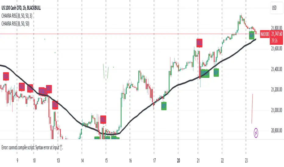
This is a scalping trading strategy built on signals from 4 EMA moving averages: EMA(8), EMA(12), EMA(24) and EMA(72).
Conditions:
- Time frame: H1 (1 hour).
- Trading assets: Applicable to major currency pairs with high volatility
- Risk management: Use a maximum of 1-2% of capital for each transaction. The order holding time can be from a few hours to a few days, depending on the price fluctuation amplitude.
Trading rules:
Determine the main trend:
Uptrend: EMA(8), EMA(12) and EMA(24) are above EMA(72).
Downtrend: EMA(8), EMA(12) and EMA(24) are below EMA(72).
Trade in the direction of the main trend** (buy in an uptrend and sell in a downtrend).
Entry conditions:
- Only trade in a clearly trending market.
Uptrend:
- Wait for the price to correct to the EMA(24).
- Enter a buy order when the price closes above the EMA(24).
- Place a stop loss below the bottom of the EMA(24) candle that has just been swept.
Downtrend:
- Wait for the price to correct to the EMA(24).
- Enter a sell order when the price closes below the EMA(24).
- Place a stop loss above the top of the EMA(24) candle that has just been swept.
Take profit and order management:
- Take profit when the price moves 20 to 40 pips in the direction of the trade.
Use Trailing Stop to optimize profits instead of setting a fixed Take Profit.
Note:
- Do not trade within 30 minutes before and after the announcement of important economic news, as the price may fluctuate abnormally.
Additional filters:
To increase the success rate and reduce noise, this strategy uses additional conditions:
1. The price is calculated only when the candle closes (no repaint).
2. When sweeping through EMA(24), the price needs to close above EMA(24).
3. The closing price must be higher than 50% of the candle's length.
4. **The bottom of the candle sweeping through EMA(24) must be lower than the bottom of the previous candle (liquidity sweep).
---
Alert function:
When the EMA(24) sweep conditions are met, the system will trigger an alert if you have set it up.
- Entry point: The closing price of the candle sweeping through EMA(24).
- Stop Loss:
- Buy Order: Place at the bottom of the sweep candle.
- Sell Order: Place at the top of the sweep candle.
---
Note:
This strategy is designed to help traders identify profitable trading opportunities based on trends. However, no strategy is 100% guaranteed to be successful. Please test it thoroughly on a demo account before using it.
Penunjuk Pine Script®