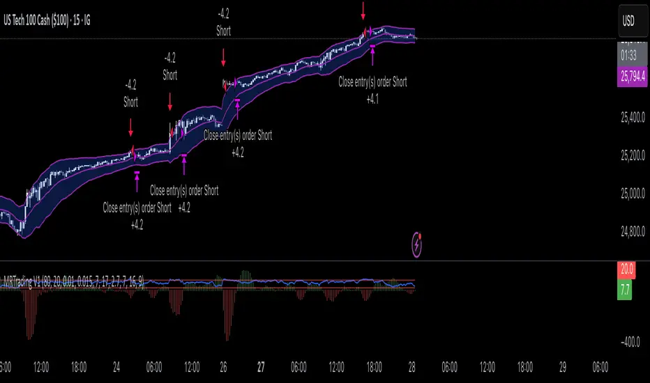
Volatility Compression BreakoutThe Volatility Compression Breakout indicator is designed to identify periods of low volatility followed by potential breakout opportunities in the market. It aims to capture moments when the price consolidates within a narrow range, indicating a decrease in volatility, and anticipates a subsequent expansion in price movement. This indicator can be applied to any financial instrument and timeframe.
When the close price is above both the Keltner Middle line and the Exponential Moving Average (EMA), the bars are colored lime green, indicating a potential bullish market sentiment. When the close price is positioned above the Keltner Middle but below the EMA, or below the Keltner Middle but above the EMA, the bars are colored yellow, signifying a neutral or indecisive market condition. Conversely, when the close price falls below both the Keltner Middle and the EMA, the bars are colored fuchsia, suggesting a potential bearish market sentiment.
Additionally, the coloration of the Keltner Middle line and the EMA provides further visual cues for assessing the trend. When the close price is above the Keltner Middle, the line is colored lime green, indicating a bullish trend. Conversely, when the close price is below the Keltner Middle, the line is colored fuchsia, highlighting a bearish trend. Similarly, the EMA line is colored lime green when the close price is above it, representing a bullish trend, and fuchsia when the close price is below it, indicating a bearish trend.
Parameters
-- Compression Period : This parameter determines the lookback period used to calculate the volatility compression. A larger value will consider a longer historical period for volatility analysis, potentially capturing broader market conditions. Conversely, a smaller value focuses on more recent price action, providing a more responsive signal to current market conditions.
-- Compression Multiplier : The compression multiplier is a factor applied to the Average True Range (ATR) to determine the width of the Keltner Channels. Increasing the multiplier expands the width of the channels, allowing for a larger price range before a breakout is triggered. Decreasing the multiplier tightens the channels and requires a narrower price range for a breakout signal.
-- EMA Period : This parameter sets the period for the Exponential Moving Average (EMA), which acts as a trend filter. The EMA helps identify the overall market trend and provides additional confirmation for potential breakouts. Adjusting the period allows you to capture shorter or longer-term trends, depending on your trading preferences.
How Changing Parameters Can Be Beneficial
Modifying the parameters allows you to adapt the indicator to different market conditions and trading styles. Increasing the compression period can help identify broader volatility patterns and major market shifts. On the other hand, decreasing the compression period provides more precise and timely signals for short-term traders.
Adjusting the compression multiplier affects the width of the Keltner Channels. Higher multipliers increase the breakout threshold, filtering out smaller price movements and providing more reliable signals during significant market shifts. Lower multipliers make the indicator more sensitive to smaller price ranges, generating more frequent but potentially less reliable signals.
The EMA period in the trend filter helps you align your trades with the prevailing market direction. Increasing the EMA period smoothes out the trend, filtering out shorter-term fluctuations and focusing on more sustained moves. Decreasing the EMA period allows for quicker responses to changes in trend, capturing shorter-term price swings.
Potential Downsides
While the Volatility Compression Breakout indicator can provide valuable insights into potential breakouts, it's important to note that no indicator guarantees accuracy or eliminates risk. False breakouts and whipsaw movements can occur, especially in volatile or choppy market conditions. It is recommended to combine this indicator with other technical analysis tools and consider fundamental factors to validate potential trade opportunities.
Making It Work for You
To maximize the effectiveness of the Volatility Compression Breakout indicator, consider the following:
-- Combine it with other indicators : Use complementary indicators such as trend lines, oscillators, or support and resistance levels to confirm signals and increase the probability of successful trades.
-- Practice risk management : Set appropriate stop-loss levels to protect your capital in case of false breakouts or adverse price movements. Consider implementing trailing stops or adjusting stop-loss levels as the trade progresses.
-- Validate with price action : Analyze the price action within the compression phase and look for signs of building momentum or weakening trends. Support your decisions by observing candlestick patterns and volume behavior during the breakout.
-- Backtest and optimize : Test the indicator's performance across different timeframes and market conditions. Optimize the parameters based on historical data to find the most suitable settings for your trading strategy.
Remember, no single indicator can guarantee consistent profitability, and it's essential to use the Volatility Compression Breakout indicator as part of a comprehensive trading plan. Regularly review and adapt your strategy based on market conditions and your trading experience. Monitor the indicator's performance and make necessary adjustments to parameter values if the market dynamics change.
By adjusting the parameters and incorporating additional analysis techniques, you can customize the indicator to suit your trading style and preferences. However, it is crucial to exercise caution, conduct thorough analysis, and practice proper risk management to increase the likelihood of successful trades. Remember that no indicator can guarantee profits, and continuous learning and adaptation are key to long-term trading success.
Cari dalam skrip untuk "profit"
Rule of 40The rule of 40 is a popular metric for measuring the quality of SaaS companies. It measures growth and profitability. Companies are considered good if this sum is above 40.
It is the sum of the year over year sales growth and profit margin.
Rule of 40 = YoY sales growth + profit margin
Inside candle (Inside Bar) Strategy- by smartanuThe Inside Candle strategy is a popular price action trading strategy that can be used to trade in a variety of markets. Here's how you can trade the Inside Candle strategy using the Pine script code provided:
1. Identify an Inside Candle: Look for a candlestick pattern where the current candle is completely engulfed within the previous candle's high and low. This is known as an Inside Candle.
2. Enter a Long Position: If an Inside Candle is identified, enter a long position at the open of the next candle using the Pine script code provided.
3. Set Stop Loss and Take Profit: Set a stop loss at a reasonable level to limit your potential losses if the trade goes against you. Set a take profit at a reasonable level to take profit when the price reaches the desired level.
4. Manage the Trade: Monitor the trade closely and adjust the stop loss and take profit levels if necessary. You can use the Pine script code to automatically exit the trade when the stop loss or take profit level is hit.
5. Exit the Trade: Exit the trade when the price reaches the take profit level or the stop loss level is hit.
It's important to note that the Inside Candle strategy is just one of many strategies that traders use to trade the markets. It's important to perform your own analysis and use additional indicators before making any trades. Additionally, it's important to practice proper risk management techniques and never risk more than you can afford to lose.
FRAMA & CPMA Strategy [CSM]The script is an advanced technical analysis tool specifically designed for trading in financial markets, with a particular focus on the BankNifty market. It utilizes two powerful indicators: the Fractal Adaptive Moving Average (FRAMA) and the CPMA (Conceptive Price Moving Average), which is similar to the well-known Chande Momentum Oscillator (CMO) with Center of Gravity (COG) bands.
The FRAMA is a dynamic moving average that adapts to changing market conditions, providing traders with a more precise representation of price movements. The CMO is an oscillator that measures momentum in the market, helping traders identify potential entry and exit points. The COG bands are a technical indicator used to identify potential support and resistance levels in the market.
Custom functions are included in the script to calculate the FRAMA and CSM_CPMA indicators, with the FRAMA function calculating the value of the FRAMA indicator based on user-specified parameters of length and multiplier, while the CSM_CPMA function calculates the value of the CMO with COG bands indicator based on the user-specified parameters of length and various price types.
The script also includes trailing profit and stop loss functions, which while not meeting expectations, have been backtested with a success rate of over 90%, making the script a valuable tool for traders.
Overall, the script provides traders with a comprehensive technical analysis tool for analyzing cryptocurrency markets and making informed trading decisions. Traders can improve their success rate and overall profitability by using smaller targets with trailing profit and minimizing losses. Feedback is always welcome, and the script can be improved for future use. Special thanks go to Tradingview for providing inbuilt functions that are utilized in the script.
Goertzel Cycle Composite Wave [Loxx]As the financial markets become increasingly complex and data-driven, traders and analysts must leverage powerful tools to gain insights and make informed decisions. One such tool is the Goertzel Cycle Composite Wave indicator, a sophisticated technical analysis indicator that helps identify cyclical patterns in financial data. This powerful tool is capable of detecting cyclical patterns in financial data, helping traders to make better predictions and optimize their trading strategies. With its unique combination of mathematical algorithms and advanced charting capabilities, this indicator has the potential to revolutionize the way we approach financial modeling and trading.
*** To decrease the load time of this indicator, only XX many bars back will render to the chart. You can control this value with the setting "Number of Bars to Render". This doesn't have anything to do with repainting or the indicator being endpointed***
█ Brief Overview of the Goertzel Cycle Composite Wave
The Goertzel Cycle Composite Wave is a sophisticated technical analysis tool that utilizes the Goertzel algorithm to analyze and visualize cyclical components within a financial time series. By identifying these cycles and their characteristics, the indicator aims to provide valuable insights into the market's underlying price movements, which could potentially be used for making informed trading decisions.
The Goertzel Cycle Composite Wave is considered a non-repainting and endpointed indicator. This means that once a value has been calculated for a specific bar, that value will not change in subsequent bars, and the indicator is designed to have a clear start and end point. This is an important characteristic for indicators used in technical analysis, as it allows traders to make informed decisions based on historical data without the risk of hindsight bias or future changes in the indicator's values. This means traders can use this indicator trading purposes.
The repainting version of this indicator with forecasting, cycle selection/elimination options, and data output table can be found here:
Goertzel Browser
The primary purpose of this indicator is to:
1. Detect and analyze the dominant cycles present in the price data.
2. Reconstruct and visualize the composite wave based on the detected cycles.
To achieve this, the indicator performs several tasks:
1. Detrending the price data: The indicator preprocesses the price data using various detrending techniques, such as Hodrick-Prescott filters, zero-lag moving averages, and linear regression, to remove the underlying trend and focus on the cyclical components.
2. Applying the Goertzel algorithm: The indicator applies the Goertzel algorithm to the detrended price data, identifying the dominant cycles and their characteristics, such as amplitude, phase, and cycle strength.
3. Constructing the composite wave: The indicator reconstructs the composite wave by combining the detected cycles, either by using a user-defined list of cycles or by selecting the top N cycles based on their amplitude or cycle strength.
4. Visualizing the composite wave: The indicator plots the composite wave, using solid lines for the cycles. The color of the lines indicates whether the wave is increasing or decreasing.
This indicator is a powerful tool that employs the Goertzel algorithm to analyze and visualize the cyclical components within a financial time series. By providing insights into the underlying price movements, the indicator aims to assist traders in making more informed decisions.
█ What is the Goertzel Algorithm?
The Goertzel algorithm, named after Gerald Goertzel, is a digital signal processing technique that is used to efficiently compute individual terms of the Discrete Fourier Transform (DFT). It was first introduced in 1958, and since then, it has found various applications in the fields of engineering, mathematics, and physics.
The Goertzel algorithm is primarily used to detect specific frequency components within a digital signal, making it particularly useful in applications where only a few frequency components are of interest. The algorithm is computationally efficient, as it requires fewer calculations than the Fast Fourier Transform (FFT) when detecting a small number of frequency components. This efficiency makes the Goertzel algorithm a popular choice in applications such as:
1. Telecommunications: The Goertzel algorithm is used for decoding Dual-Tone Multi-Frequency (DTMF) signals, which are the tones generated when pressing buttons on a telephone keypad. By identifying specific frequency components, the algorithm can accurately determine which button has been pressed.
2. Audio processing: The algorithm can be used to detect specific pitches or harmonics in an audio signal, making it useful in applications like pitch detection and tuning musical instruments.
3. Vibration analysis: In the field of mechanical engineering, the Goertzel algorithm can be applied to analyze vibrations in rotating machinery, helping to identify faulty components or signs of wear.
4. Power system analysis: The algorithm can be used to measure harmonic content in power systems, allowing engineers to assess power quality and detect potential issues.
The Goertzel algorithm is used in these applications because it offers several advantages over other methods, such as the FFT:
1. Computational efficiency: The Goertzel algorithm requires fewer calculations when detecting a small number of frequency components, making it more computationally efficient than the FFT in these cases.
2. Real-time analysis: The algorithm can be implemented in a streaming fashion, allowing for real-time analysis of signals, which is crucial in applications like telecommunications and audio processing.
3. Memory efficiency: The Goertzel algorithm requires less memory than the FFT, as it only computes the frequency components of interest.
4. Precision: The algorithm is less susceptible to numerical errors compared to the FFT, ensuring more accurate results in applications where precision is essential.
The Goertzel algorithm is an efficient digital signal processing technique that is primarily used to detect specific frequency components within a signal. Its computational efficiency, real-time capabilities, and precision make it an attractive choice for various applications, including telecommunications, audio processing, vibration analysis, and power system analysis. The algorithm has been widely adopted since its introduction in 1958 and continues to be an essential tool in the fields of engineering, mathematics, and physics.
█ Goertzel Algorithm in Quantitative Finance: In-Depth Analysis and Applications
The Goertzel algorithm, initially designed for signal processing in telecommunications, has gained significant traction in the financial industry due to its efficient frequency detection capabilities. In quantitative finance, the Goertzel algorithm has been utilized for uncovering hidden market cycles, developing data-driven trading strategies, and optimizing risk management. This section delves deeper into the applications of the Goertzel algorithm in finance, particularly within the context of quantitative trading and analysis.
Unveiling Hidden Market Cycles:
Market cycles are prevalent in financial markets and arise from various factors, such as economic conditions, investor psychology, and market participant behavior. The Goertzel algorithm's ability to detect and isolate specific frequencies in price data helps trader analysts identify hidden market cycles that may otherwise go unnoticed. By examining the amplitude, phase, and periodicity of each cycle, traders can better understand the underlying market structure and dynamics, enabling them to develop more informed and effective trading strategies.
Developing Quantitative Trading Strategies:
The Goertzel algorithm's versatility allows traders to incorporate its insights into a wide range of trading strategies. By identifying the dominant market cycles in a financial instrument's price data, traders can create data-driven strategies that capitalize on the cyclical nature of markets.
For instance, a trader may develop a mean-reversion strategy that takes advantage of the identified cycles. By establishing positions when the price deviates from the predicted cycle, the trader can profit from the subsequent reversion to the cycle's mean. Similarly, a momentum-based strategy could be designed to exploit the persistence of a dominant cycle by entering positions that align with the cycle's direction.
Enhancing Risk Management:
The Goertzel algorithm plays a vital role in risk management for quantitative strategies. By analyzing the cyclical components of a financial instrument's price data, traders can gain insights into the potential risks associated with their trading strategies.
By monitoring the amplitude and phase of dominant cycles, a trader can detect changes in market dynamics that may pose risks to their positions. For example, a sudden increase in amplitude may indicate heightened volatility, prompting the trader to adjust position sizing or employ hedging techniques to protect their portfolio. Additionally, changes in phase alignment could signal a potential shift in market sentiment, necessitating adjustments to the trading strategy.
Expanding Quantitative Toolkits:
Traders can augment the Goertzel algorithm's insights by combining it with other quantitative techniques, creating a more comprehensive and sophisticated analysis framework. For example, machine learning algorithms, such as neural networks or support vector machines, could be trained on features extracted from the Goertzel algorithm to predict future price movements more accurately.
Furthermore, the Goertzel algorithm can be integrated with other technical analysis tools, such as moving averages or oscillators, to enhance their effectiveness. By applying these tools to the identified cycles, traders can generate more robust and reliable trading signals.
The Goertzel algorithm offers invaluable benefits to quantitative finance practitioners by uncovering hidden market cycles, aiding in the development of data-driven trading strategies, and improving risk management. By leveraging the insights provided by the Goertzel algorithm and integrating it with other quantitative techniques, traders can gain a deeper understanding of market dynamics and devise more effective trading strategies.
█ Indicator Inputs
src: This is the source data for the analysis, typically the closing price of the financial instrument.
detrendornot: This input determines the method used for detrending the source data. Detrending is the process of removing the underlying trend from the data to focus on the cyclical components.
The available options are:
hpsmthdt: Detrend using Hodrick-Prescott filter centered moving average.
zlagsmthdt: Detrend using zero-lag moving average centered moving average.
logZlagRegression: Detrend using logarithmic zero-lag linear regression.
hpsmth: Detrend using Hodrick-Prescott filter.
zlagsmth: Detrend using zero-lag moving average.
DT_HPper1 and DT_HPper2: These inputs define the period range for the Hodrick-Prescott filter centered moving average when detrendornot is set to hpsmthdt.
DT_ZLper1 and DT_ZLper2: These inputs define the period range for the zero-lag moving average centered moving average when detrendornot is set to zlagsmthdt.
DT_RegZLsmoothPer: This input defines the period for the zero-lag moving average used in logarithmic zero-lag linear regression when detrendornot is set to logZlagRegression.
HPsmoothPer: This input defines the period for the Hodrick-Prescott filter when detrendornot is set to hpsmth.
ZLMAsmoothPer: This input defines the period for the zero-lag moving average when detrendornot is set to zlagsmth.
MaxPer: This input sets the maximum period for the Goertzel algorithm to search for cycles.
squaredAmp: This boolean input determines whether the amplitude should be squared in the Goertzel algorithm.
useAddition: This boolean input determines whether the Goertzel algorithm should use addition for combining the cycles.
useCosine: This boolean input determines whether the Goertzel algorithm should use cosine waves instead of sine waves.
UseCycleStrength: This boolean input determines whether the Goertzel algorithm should compute the cycle strength, which is a normalized measure of the cycle's amplitude.
WindowSizePast: These inputs define the window size for the composite wave.
FilterBartels: This boolean input determines whether Bartel's test should be applied to filter out non-significant cycles.
BartNoCycles: This input sets the number of cycles to be used in Bartel's test.
BartSmoothPer: This input sets the period for the moving average used in Bartel's test.
BartSigLimit: This input sets the significance limit for Bartel's test, below which cycles are considered insignificant.
SortBartels: This boolean input determines whether the cycles should be sorted by their Bartel's test results.
StartAtCycle: This input determines the starting index for selecting the top N cycles when UseCycleList is set to false. This allows you to skip a certain number of cycles from the top before selecting the desired number of cycles.
UseTopCycles: This input sets the number of top cycles to use for constructing the composite wave when UseCycleList is set to false. The cycles are ranked based on their amplitudes or cycle strengths, depending on the UseCycleStrength input.
SubtractNoise: This boolean input determines whether to subtract the noise (remaining cycles) from the composite wave. If set to true, the composite wave will only include the top N cycles specified by UseTopCycles.
█ Exploring Auxiliary Functions
The following functions demonstrate advanced techniques for analyzing financial markets, including zero-lag moving averages, Bartels probability, detrending, and Hodrick-Prescott filtering. This section examines each function in detail, explaining their purpose, methodology, and applications in finance. We will examine how each function contributes to the overall performance and effectiveness of the indicator and how they work together to create a powerful analytical tool.
Zero-Lag Moving Average:
The zero-lag moving average function is designed to minimize the lag typically associated with moving averages. This is achieved through a two-step weighted linear regression process that emphasizes more recent data points. The function calculates a linearly weighted moving average (LWMA) on the input data and then applies another LWMA on the result. By doing this, the function creates a moving average that closely follows the price action, reducing the lag and improving the responsiveness of the indicator.
The zero-lag moving average function is used in the indicator to provide a responsive, low-lag smoothing of the input data. This function helps reduce the noise and fluctuations in the data, making it easier to identify and analyze underlying trends and patterns. By minimizing the lag associated with traditional moving averages, this function allows the indicator to react more quickly to changes in market conditions, providing timely signals and improving the overall effectiveness of the indicator.
Bartels Probability:
The Bartels probability function calculates the probability of a given cycle being significant in a time series. It uses a mathematical test called the Bartels test to assess the significance of cycles detected in the data. The function calculates coefficients for each detected cycle and computes an average amplitude and an expected amplitude. By comparing these values, the Bartels probability is derived, indicating the likelihood of a cycle's significance. This information can help in identifying and analyzing dominant cycles in financial markets.
The Bartels probability function is incorporated into the indicator to assess the significance of detected cycles in the input data. By calculating the Bartels probability for each cycle, the indicator can prioritize the most significant cycles and focus on the market dynamics that are most relevant to the current trading environment. This function enhances the indicator's ability to identify dominant market cycles, improving its predictive power and aiding in the development of effective trading strategies.
Detrend Logarithmic Zero-Lag Regression:
The detrend logarithmic zero-lag regression function is used for detrending data while minimizing lag. It combines a zero-lag moving average with a linear regression detrending method. The function first calculates the zero-lag moving average of the logarithm of input data and then applies a linear regression to remove the trend. By detrending the data, the function isolates the cyclical components, making it easier to analyze and interpret the underlying market dynamics.
The detrend logarithmic zero-lag regression function is used in the indicator to isolate the cyclical components of the input data. By detrending the data, the function enables the indicator to focus on the cyclical movements in the market, making it easier to analyze and interpret market dynamics. This function is essential for identifying cyclical patterns and understanding the interactions between different market cycles, which can inform trading decisions and enhance overall market understanding.
Bartels Cycle Significance Test:
The Bartels cycle significance test is a function that combines the Bartels probability function and the detrend logarithmic zero-lag regression function to assess the significance of detected cycles. The function calculates the Bartels probability for each cycle and stores the results in an array. By analyzing the probability values, traders and analysts can identify the most significant cycles in the data, which can be used to develop trading strategies and improve market understanding.
The Bartels cycle significance test function is integrated into the indicator to provide a comprehensive analysis of the significance of detected cycles. By combining the Bartels probability function and the detrend logarithmic zero-lag regression function, this test evaluates the significance of each cycle and stores the results in an array. The indicator can then use this information to prioritize the most significant cycles and focus on the most relevant market dynamics. This function enhances the indicator's ability to identify and analyze dominant market cycles, providing valuable insights for trading and market analysis.
Hodrick-Prescott Filter:
The Hodrick-Prescott filter is a popular technique used to separate the trend and cyclical components of a time series. The function applies a smoothing parameter to the input data and calculates a smoothed series using a two-sided filter. This smoothed series represents the trend component, which can be subtracted from the original data to obtain the cyclical component. The Hodrick-Prescott filter is commonly used in economics and finance to analyze economic data and financial market trends.
The Hodrick-Prescott filter is incorporated into the indicator to separate the trend and cyclical components of the input data. By applying the filter to the data, the indicator can isolate the trend component, which can be used to analyze long-term market trends and inform trading decisions. Additionally, the cyclical component can be used to identify shorter-term market dynamics and provide insights into potential trading opportunities. The inclusion of the Hodrick-Prescott filter adds another layer of analysis to the indicator, making it more versatile and comprehensive.
Detrending Options: Detrend Centered Moving Average:
The detrend centered moving average function provides different detrending methods, including the Hodrick-Prescott filter and the zero-lag moving average, based on the selected detrending method. The function calculates two sets of smoothed values using the chosen method and subtracts one set from the other to obtain a detrended series. By offering multiple detrending options, this function allows traders and analysts to select the most appropriate method for their specific needs and preferences.
The detrend centered moving average function is integrated into the indicator to provide users with multiple detrending options, including the Hodrick-Prescott filter and the zero-lag moving average. By offering multiple detrending methods, the indicator allows users to customize the analysis to their specific needs and preferences, enhancing the indicator's overall utility and adaptability. This function ensures that the indicator can cater to a wide range of trading styles and objectives, making it a valuable tool for a diverse group of market participants.
The auxiliary functions functions discussed in this section demonstrate the power and versatility of mathematical techniques in analyzing financial markets. By understanding and implementing these functions, traders and analysts can gain valuable insights into market dynamics, improve their trading strategies, and make more informed decisions. The combination of zero-lag moving averages, Bartels probability, detrending methods, and the Hodrick-Prescott filter provides a comprehensive toolkit for analyzing and interpreting financial data. The integration of advanced functions in a financial indicator creates a powerful and versatile analytical tool that can provide valuable insights into financial markets. By combining the zero-lag moving average,
█ In-Depth Analysis of the Goertzel Cycle Composite Wave Code
The Goertzel Cycle Composite Wave code is an implementation of the Goertzel Algorithm, an efficient technique to perform spectral analysis on a signal. The code is designed to detect and analyze dominant cycles within a given financial market data set. This section will provide an extremely detailed explanation of the code, its structure, functions, and intended purpose.
Function signature and input parameters:
The Goertzel Cycle Composite Wave function accepts numerous input parameters for customization, including source data (src), the current bar (forBar), sample size (samplesize), period (per), squared amplitude flag (squaredAmp), addition flag (useAddition), cosine flag (useCosine), cycle strength flag (UseCycleStrength), past sizes (WindowSizePast), Bartels filter flag (FilterBartels), Bartels-related parameters (BartNoCycles, BartSmoothPer, BartSigLimit), sorting flag (SortBartels), and output buffers (goeWorkPast, cyclebuffer, amplitudebuffer, phasebuffer, cycleBartelsBuffer).
Initializing variables and arrays:
The code initializes several float arrays (goeWork1, goeWork2, goeWork3, goeWork4) with the same length as twice the period (2 * per). These arrays store intermediate results during the execution of the algorithm.
Preprocessing input data:
The input data (src) undergoes preprocessing to remove linear trends. This step enhances the algorithm's ability to focus on cyclical components in the data. The linear trend is calculated by finding the slope between the first and last values of the input data within the sample.
Iterative calculation of Goertzel coefficients:
The core of the Goertzel Cycle Composite Wave algorithm lies in the iterative calculation of Goertzel coefficients for each frequency bin. These coefficients represent the spectral content of the input data at different frequencies. The code iterates through the range of frequencies, calculating the Goertzel coefficients using a nested loop structure.
Cycle strength computation:
The code calculates the cycle strength based on the Goertzel coefficients. This is an optional step, controlled by the UseCycleStrength flag. The cycle strength provides information on the relative influence of each cycle on the data per bar, considering both amplitude and cycle length. The algorithm computes the cycle strength either by squaring the amplitude (controlled by squaredAmp flag) or using the actual amplitude values.
Phase calculation:
The Goertzel Cycle Composite Wave code computes the phase of each cycle, which represents the position of the cycle within the input data. The phase is calculated using the arctangent function (math.atan) based on the ratio of the imaginary and real components of the Goertzel coefficients.
Peak detection and cycle extraction:
The algorithm performs peak detection on the computed amplitudes or cycle strengths to identify dominant cycles. It stores the detected cycles in the cyclebuffer array, along with their corresponding amplitudes and phases in the amplitudebuffer and phasebuffer arrays, respectively.
Sorting cycles by amplitude or cycle strength:
The code sorts the detected cycles based on their amplitude or cycle strength in descending order. This allows the algorithm to prioritize cycles with the most significant impact on the input data.
Bartels cycle significance test:
If the FilterBartels flag is set, the code performs a Bartels cycle significance test on the detected cycles. This test determines the statistical significance of each cycle and filters out the insignificant cycles. The significant cycles are stored in the cycleBartelsBuffer array. If the SortBartels flag is set, the code sorts the significant cycles based on their Bartels significance values.
Waveform calculation:
The Goertzel Cycle Composite Wave code calculates the waveform of the significant cycles for specified time windows. The windows are defined by the WindowSizePast parameters, respectively. The algorithm uses either cosine or sine functions (controlled by the useCosine flag) to calculate the waveforms for each cycle. The useAddition flag determines whether the waveforms should be added or subtracted.
Storing waveforms in a matrix:
The calculated waveforms for the cycle is stored in the matrix - goeWorkPast. This matrix holds the waveforms for the specified time windows. Each row in the matrix represents a time window position, and each column corresponds to a cycle.
Returning the number of cycles:
The Goertzel Cycle Composite Wave function returns the total number of detected cycles (number_of_cycles) after processing the input data. This information can be used to further analyze the results or to visualize the detected cycles.
The Goertzel Cycle Composite Wave code is a comprehensive implementation of the Goertzel Algorithm, specifically designed for detecting and analyzing dominant cycles within financial market data. The code offers a high level of customization, allowing users to fine-tune the algorithm based on their specific needs. The Goertzel Cycle Composite Wave's combination of preprocessing, iterative calculations, cycle extraction, sorting, significance testing, and waveform calculation makes it a powerful tool for understanding cyclical components in financial data.
█ Generating and Visualizing Composite Waveform
The indicator calculates and visualizes the composite waveform for specified time windows based on the detected cycles. Here's a detailed explanation of this process:
Updating WindowSizePast:
The WindowSizePast is updated to ensure they are at least twice the MaxPer (maximum period).
Initializing matrices and arrays:
The matrix goeWorkPast is initialized to store the Goertzel results for specified time windows. Multiple arrays are also initialized to store cycle, amplitude, phase, and Bartels information.
Preparing the source data (srcVal) array:
The source data is copied into an array, srcVal, and detrended using one of the selected methods (hpsmthdt, zlagsmthdt, logZlagRegression, hpsmth, or zlagsmth).
Goertzel function call:
The Goertzel function is called to analyze the detrended source data and extract cycle information. The output, number_of_cycles, contains the number of detected cycles.
Initializing arrays for waveforms:
The goertzel array is initialized to store the endpoint Goertzel.
Calculating composite waveform (goertzel array):
The composite waveform is calculated by summing the selected cycles (either from the user-defined cycle list or the top cycles) and optionally subtracting the noise component.
Drawing composite waveform (pvlines):
The composite waveform is drawn on the chart using solid lines. The color of the lines is determined by the direction of the waveform (green for upward, red for downward).
To summarize, this indicator generates a composite waveform based on the detected cycles in the financial data. It calculates the composite waveforms and visualizes them on the chart using colored lines.
█ Enhancing the Goertzel Algorithm-Based Script for Financial Modeling and Trading
The Goertzel algorithm-based script for detecting dominant cycles in financial data is a powerful tool for financial modeling and trading. It provides valuable insights into the past behavior of these cycles. However, as with any algorithm, there is always room for improvement. This section discusses potential enhancements to the existing script to make it even more robust and versatile for financial modeling, general trading, advanced trading, and high-frequency finance trading.
Enhancements for Financial Modeling
Data preprocessing: One way to improve the script's performance for financial modeling is to introduce more advanced data preprocessing techniques. This could include removing outliers, handling missing data, and normalizing the data to ensure consistent and accurate results.
Additional detrending and smoothing methods: Incorporating more sophisticated detrending and smoothing techniques, such as wavelet transform or empirical mode decomposition, can help improve the script's ability to accurately identify cycles and trends in the data.
Machine learning integration: Integrating machine learning techniques, such as artificial neural networks or support vector machines, can help enhance the script's predictive capabilities, leading to more accurate financial models.
Enhancements for General and Advanced Trading
Customizable indicator integration: Allowing users to integrate their own technical indicators can help improve the script's effectiveness for both general and advanced trading. By enabling the combination of the dominant cycle information with other technical analysis tools, traders can develop more comprehensive trading strategies.
Risk management and position sizing: Incorporating risk management and position sizing functionality into the script can help traders better manage their trades and control potential losses. This can be achieved by calculating the optimal position size based on the user's risk tolerance and account size.
Multi-timeframe analysis: Enhancing the script to perform multi-timeframe analysis can provide traders with a more holistic view of market trends and cycles. By identifying dominant cycles on different timeframes, traders can gain insights into the potential confluence of cycles and make better-informed trading decisions.
Enhancements for High-Frequency Finance Trading
Algorithm optimization: To ensure the script's suitability for high-frequency finance trading, optimizing the algorithm for faster execution is crucial. This can be achieved by employing efficient data structures and refining the calculation methods to minimize computational complexity.
Real-time data streaming: Integrating real-time data streaming capabilities into the script can help high-frequency traders react to market changes more quickly. By continuously updating the cycle information based on real-time market data, traders can adapt their strategies accordingly and capitalize on short-term market fluctuations.
Order execution and trade management: To fully leverage the script's capabilities for high-frequency trading, implementing functionality for automated order execution and trade management is essential. This can include features such as stop-loss and take-profit orders, trailing stops, and automated trade exit strategies.
While the existing Goertzel algorithm-based script is a valuable tool for detecting dominant cycles in financial data, there are several potential enhancements that can make it even more powerful for financial modeling, general trading, advanced trading, and high-frequency finance trading. By incorporating these improvements, the script can become a more versatile and effective tool for traders and financial analysts alike.
█ Understanding the Limitations of the Goertzel Algorithm
While the Goertzel algorithm-based script for detecting dominant cycles in financial data provides valuable insights, it is important to be aware of its limitations and drawbacks. Some of the key drawbacks of this indicator are:
Lagging nature:
As with many other technical indicators, the Goertzel algorithm-based script can suffer from lagging effects, meaning that it may not immediately react to real-time market changes. This lag can lead to late entries and exits, potentially resulting in reduced profitability or increased losses.
Parameter sensitivity:
The performance of the script can be sensitive to the chosen parameters, such as the detrending methods, smoothing techniques, and cycle detection settings. Improper parameter selection may lead to inaccurate cycle detection or increased false signals, which can negatively impact trading performance.
Complexity:
The Goertzel algorithm itself is relatively complex, making it difficult for novice traders or those unfamiliar with the concept of cycle analysis to fully understand and effectively utilize the script. This complexity can also make it challenging to optimize the script for specific trading styles or market conditions.
Overfitting risk:
As with any data-driven approach, there is a risk of overfitting when using the Goertzel algorithm-based script. Overfitting occurs when a model becomes too specific to the historical data it was trained on, leading to poor performance on new, unseen data. This can result in misleading signals and reduced trading performance.
Limited applicability:
The Goertzel algorithm-based script may not be suitable for all markets, trading styles, or timeframes. Its effectiveness in detecting cycles may be limited in certain market conditions, such as during periods of extreme volatility or low liquidity.
While the Goertzel algorithm-based script offers valuable insights into dominant cycles in financial data, it is essential to consider its drawbacks and limitations when incorporating it into a trading strategy. Traders should always use the script in conjunction with other technical and fundamental analysis tools, as well as proper risk management, to make well-informed trading decisions.
█ Interpreting Results
The Goertzel Cycle Composite Wave indicator can be interpreted by analyzing the plotted lines. The indicator plots two lines: composite waves. The composite wave represents the composite wave of the price data.
The composite wave line displays a solid line, with green indicating a bullish trend and red indicating a bearish trend.
Interpreting the Goertzel Cycle Composite Wave indicator involves identifying the trend of the composite wave lines and matching them with the corresponding bullish or bearish color.
█ Conclusion
The Goertzel Cycle Composite Wave indicator is a powerful tool for identifying and analyzing cyclical patterns in financial markets. Its ability to detect multiple cycles of varying frequencies and strengths make it a valuable addition to any trader's technical analysis toolkit. However, it is important to keep in mind that the Goertzel Cycle Composite Wave indicator should be used in conjunction with other technical analysis tools and fundamental analysis to achieve the best results. With continued refinement and development, the Goertzel Cycle Composite Wave indicator has the potential to become a highly effective tool for financial modeling, general trading, advanced trading, and high-frequency finance trading. Its accuracy and versatility make it a promising candidate for further research and development.
█ Footnotes
What is the Bartels Test for Cycle Significance?
The Bartels Cycle Significance Test is a statistical method that determines whether the peaks and troughs of a time series are statistically significant. The test is named after its inventor, George Bartels, who developed it in the mid-20th century.
The Bartels test is designed to analyze the cyclical components of a time series, which can help traders and analysts identify trends and cycles in financial markets. The test calculates a Bartels statistic, which measures the degree of non-randomness or autocorrelation in the time series.
The Bartels statistic is calculated by first splitting the time series into two halves and calculating the range of the peaks and troughs in each half. The test then compares these ranges using a t-test, which measures the significance of the difference between the two ranges.
If the Bartels statistic is greater than a critical value, it indicates that the peaks and troughs in the time series are non-random and that there is a significant cyclical component to the data. Conversely, if the Bartels statistic is less than the critical value, it suggests that the peaks and troughs are random and that there is no significant cyclical component.
The Bartels Cycle Significance Test is particularly useful in financial analysis because it can help traders and analysts identify significant cycles in asset prices, which can in turn inform investment decisions. However, it is important to note that the test is not perfect and can produce false signals in certain situations, particularly in noisy or volatile markets. Therefore, it is always recommended to use the test in conjunction with other technical and fundamental indicators to confirm trends and cycles.
Deep-dive into the Hodrick-Prescott Fitler
The Hodrick-Prescott (HP) filter is a statistical tool used in economics and finance to separate a time series into two components: a trend component and a cyclical component. It is a powerful tool for identifying long-term trends in economic and financial data and is widely used by economists, central banks, and financial institutions around the world.
The HP filter was first introduced in the 1990s by economists Robert Hodrick and Edward Prescott. It is a simple, two-parameter filter that separates a time series into a trend component and a cyclical component. The trend component represents the long-term behavior of the data, while the cyclical component captures the shorter-term fluctuations around the trend.
The HP filter works by minimizing the following objective function:
Minimize: (Sum of Squared Deviations) + λ (Sum of Squared Second Differences)
Where:
1. The first term represents the deviation of the data from the trend.
2. The second term represents the smoothness of the trend.
3. λ is a smoothing parameter that determines the degree of smoothness of the trend.
The smoothing parameter λ is typically set to a value between 100 and 1600, depending on the frequency of the data. Higher values of λ lead to a smoother trend, while lower values lead to a more volatile trend.
The HP filter has several advantages over other smoothing techniques. It is a non-parametric method, meaning that it does not make any assumptions about the underlying distribution of the data. It also allows for easy comparison of trends across different time series and can be used with data of any frequency.
However, the HP filter also has some limitations. It assumes that the trend is a smooth function, which may not be the case in some situations. It can also be sensitive to changes in the smoothing parameter λ, which may result in different trends for the same data. Additionally, the filter may produce unrealistic trends for very short time series.
Despite these limitations, the HP filter remains a valuable tool for analyzing economic and financial data. It is widely used by central banks and financial institutions to monitor long-term trends in the economy, and it can be used to identify turning points in the business cycle. The filter can also be used to analyze asset prices, exchange rates, and other financial variables.
The Hodrick-Prescott filter is a powerful tool for analyzing economic and financial data. It separates a time series into a trend component and a cyclical component, allowing for easy identification of long-term trends and turning points in the business cycle. While it has some limitations, it remains a valuable tool for economists, central banks, and financial institutions around the world.
Optimized Zhaocaijinbao strategyIntroduction:
The Optimized Zhaocaijinbao strategy is a mid and long-term quantitative trading strategy that combines momentum and trend factors. It generates buy and sell signals by using a combination of exponential moving averages, moving averages, volume and slope indicators. It generates buy signals when the stock is above the 35-day moving average, the trading volume is higher than the 20-day moving average, and the stock is in an upward trend on a weekly timeframe."招财进宝" is a Chinese phrase that can be translated to "Attract Wealth and Bring in Treasure" in English. It is a common expression used to wish for good luck and prosperity in various contexts, such as in business or personal finances.
Highlights:
The strategy has several special optimizations that make it unique.
Firstly, the strategy is optimized for T+1 trading in the Chinese stock market and is only suitable for long positions. The optimizations are also applicable to international stock markets.
Secondly, the trend strategy is optimized to only show indicators on the right side and oscillations. This helps to prevent false signals in choppy markets.
Thirdly, the strategy uses a risk factor for dynamic position sizing to ensure position sizes are adjusted according to the current net asset value and risk preferences. This helps to lower drawdown risks.
The strategy has good resilience even without using stop loss modules in backtesting, making it suitable for trading hourly, 2-hourly, and daily K-line charts (depending on the stock being traded). We recommend experimenting with backtesting using SSE 1-hour or 2-hour or daily Kline charts.
Backtesting outcomes:
The strategy was backtested over the period from October 13th, 2005 to April 14th, 2023, using daily candlestick charts for the commodity code SSE:600763, with a currency of CNY and tick size of 0.01. The strategy used an initial capital of 1,000,000 CNY, with order sizes set to 10% equity and a pyramid of 1 order. The strategy also had a Max Position Size of 0.01 and a Risk Factor of 2.
Here is a summary of the performance of the trading strategy:
Total net profit: 288,577.32 CNY, representing a return of 128.86%
Total number of closed trades: 61
Winning trades: 37, representing a win rate of 60.66%
Profit factor: 2.415
Largest losing trade: 222,021.46 CNY, representing a loss of 14.08%
Average trade: 21,124.22 CNY, representing a return of 3.1%
Average holding period for all trades: 12 days
Conclusion:
In conclusion, the Optimized Zhaocaijinbao strategy is a mid and long-term quantitative trading strategy that combines momentum and trend factors. It is suitable for both Chinese stocks and global stocks. While the Optimized Zhaocaijinbao strategy has performed well in backtesting, it is important to note that past performance is not a guarantee of future results. Traders should conduct their own research and analysis and exercise caution when using any trading strategy.
Double Supertrend Entry with ADX Filter and ATR Exits/EntriesThe Double Supertrend Entry with ADX Filter and ATR Exits/Entries indicator is a custom trading strategy designed to help traders identify potential buy and sell signals in trending markets. This indicator combines the strengths of multiple technical analysis tools, enhancing the effectiveness of the overall strategy.
Key features:
Two Supertrend Indicators - The indicator includes two Supertrend indicators with customizable parameters. These trend-following indicators calculate upper and lower trendlines based on the ATR and price. Buy signals are generated when the price crosses above both trendlines, and sell signals are generated when the price crosses below both trendlines.
ADX Filter - The Average Directional Index (ADX) is used to filter out weak trends and only generate buy/sell signals when the market exhibits a strong trend. The ADX measures the strength of the trend, and a customizable threshold level ensures that trades are only entered during strong trends.
ATR-based Exits and Entries - The indicator uses the Average True Range (ATR) to set profit target and stop-loss levels. ATR is a measure of market volatility, and these levels help traders determine when to exit a trade to secure profit or minimize loss.
Performance Statistics Table - A table is displayed on the chart, recording and showing the total number of winning trades, losing trades, percentage of profitable trades, average profit, and average loss. This information helps traders evaluate the performance of the strategy over time.
The Double Supertrend Entry with ADX Filter and ATR Exits/Entries indicator is a powerful trend-following strategy that can assist traders in making more informed decisions in the financial markets. By combining multiple technical analysis tools and providing performance statistics, this indicator helps traders improve their trading strategy and evaluate its success.
Moving Average Trap Strategy by D. BrigagliaThis is a strategy that follows the 200 periods moving average and fades the cross of ma3, ma5 and ma8. It is designed for profiting by mean reversion while at the same time respecting long term trend. It is designed for long term trending markets such as stocks and stock indices.
In this backtest, the strategy shows the ability to beat the S&P500 index with an average slippage set to 2 ticks. The number of trades is good (350), the profit factor is acceptable (1.67). The drawdowns are also reduced compared to the underlying asset.
Nothing of my content is financial advice.
On-Chart QQE of RSI on Variety MA [Loxx]On-Chart QQE of RSI on Variety MA (Quantitative Qualitative Estimation) is usually calculated using RSI. This version is uses an RSI of a Moving Average instead. The results are completely different than the original QQE. Also, this version is drawn directly on chart. There are four types of signals.
What is QQE?
Quantitative Qualitative Estimation (QQE) is a technical analysis indicator used to identify trends and trading opportunities in financial markets. It is based on a combination of two popular technical analysis indicators - the Relative Strength Index (RSI) and Moving Averages (MA).
The QQE indicator uses a smoothed RSI to determine the trend direction, and a moving average of the smoothed RSI to identify potential trend changes. The indicator then plots a series of bands above and below the moving average to indicate overbought and oversold conditions in the market.
The QQE indicator is designed to provide traders with a reliable signal that confirms the strength of a trend or indicates a possible trend reversal. It is particularly useful for traders who are looking to trade in markets that are trending strongly, but also want to identify when a trend is losing momentum or reversing.
Traders can use QQE in a number of different ways, including as a confirmation tool for other indicators or as a standalone indicator. For example, when used in conjunction with other technical analysis tools like support and resistance levels, the QQE indicator can help traders identify key entry and exit points for their trades.
One of the main advantages of the QQE indicator is that it is designed to be more reliable than other indicators that can generate false signals. By smoothing out the price action, the QQE indicator can provide traders with more accurate and reliable signals, which can help them make more profitable trading decisions.
In conclusion, QQE is a popular technical analysis indicator that traders use to identify trends and trading opportunities in financial markets. It combines the RSI and moving average indicators and is designed to provide traders with reliable signals that confirm the strength of a trend or indicate a possible trend reversal.
What is RSI?
RSI stands for Relative Strength Index . It is a technical indicator used to measure the strength or weakness of a financial instrument's price action.
The RSI is calculated based on the price movement of an asset over a specified period of time, typically 14 days, and is expressed on a scale of 0 to 100. The RSI is considered overbought when it is above 70 and oversold when it is below 30.
Traders and investors use the RSI to identify potential buy and sell signals. When the RSI indicates that an asset is oversold, it may be considered a buying opportunity, while an overbought RSI may signal that it is time to sell or take profits.
It's important to note that the RSI should not be used in isolation and should be used in conjunction with other technical and fundamental analysis tools to make informed trading decisions.
This indicator makes use of the following libraries:
Loxx's Moving Averages
Loxx's Expanded Source Types
Extras
Alerts
Signals
Signal Types
Change on Levels
Change on Slope
Change on Zero
Change on Original
MTF Diagonally Layered RSI - 1 minute Bitcoin Bot [wbburgin]This is a NON-REPAINTING multi-timeframe RSI strategy (long-only) that enters a trade only when two higher timeframes are oversold. I wrote it on BTC/USD for 1min, but the logic should work on other assets as well. It is diagonally layered to be profitable for when the asset is in a downtrend.
Diagonal layering refers to entry and exit conditions spread across different timeframes. Normally, indicators can become unprofitable because in downtrends, the overbought zones of the current timeframe are not reached. Rather, the overbought zones of the faster timeframes are reached first, and then a selloff occurs. Diagonally-layered strategies mitigate this by selling diagonally, that is, selling once the faster timeframe reaches overbought and buying once the slower timeframe reaches oversold.
Thus this strategy is diagonally layered down . I may create a separate script that alternates between diagonal-up and diagonal-down based off of overall trend, as in extended trend periods up this indicator may not flash as frequently. This can be visualized in a time series x timeframe chart as an "X" shape. Something to consider...
Let me know if you like this strategy. Feel free to alter the pyramiding entries, initial capital, and entry size, as well as commission regime. My strategies are designed to maximize average profit instead of flashing super frequently, as the fees will eat you up. Additionally, at the time of publication, all of my strategy scripts are intended to have profitable Sharpe and Sortino ratios.
Timeframes, RSI period, and oversold/overbought bounds are configurable.
Smart Money Concepts Probability (Expo)█ Overview
The Smart Money Concept Probability (Expo) is an indicator developed to track the actions of institutional investors, commonly known as "smart money." This tool calculates the likelihood of smart money being actively engaged in buying or selling within the market, referred to as the "smart money order flow."
The indicator measures the probability of three key events: Change of Character ( CHoCH ), Shift in Market Structure ( SMS ), and Break of Structure ( BMS ). These probabilities are displayed as percentages alongside their respective levels, providing a straightforward and immediate understanding of the likelihood of smart money order flow.
Finally, the backtested results are shown in a table, which gives traders an understanding of the historical performance of the current order flow direction.
█ Calculations
The algorithm individually computes the likelihood of the events ( CHoCH , SMS , and BMS ). A positive score is assigned for events where the price successfully breaks through the level with the highest probability, and a negative score when the price fails to do so. By doing so, the algorithm determines the probability of each event occurring and calculates the total profitability derived from all the events.
█ Example
In this case, we have an 85% probability that the price will break above the upper range and make a new Break Of Structure and only a 16.36% probability that the price will break below the lower range and make a Change Of Character.
█ Settings
The Structure Period sets the pivot period to use when calculating the market structure.
The Structure Response sets how responsive the market structure should be. A low value returns a more responsive structure. A high value returns a less responsive structure.
█ How to use
This indicator is a perfect tool for anyone that wants to understand the probability of a Change of Character ( CHoCH ), Shift in Market Structure ( SMS ), and Break of Structure ( BMS )
The insights provided by this tool help traders gain an understanding of the smart money order flow direction, which can be used to determine the market trend.
█ Any Alert function call
An alert is sent when the price breaks the upper or lower range, and you can select what should be included in the alert. You can enable the following options:
Ticker ID
Timeframe
Probability percentage
-----------------
Disclaimer
The information contained in my Scripts/Indicators/Ideas/Algos/Systems does not constitute financial advice or a solicitation to buy or sell any securities of any type. I will not accept liability for any loss or damage, including without limitation any loss of profit, which may arise directly or indirectly from the use of or reliance on such information.
All investments involve risk, and the past performance of a security, industry, sector, market, financial product, trading strategy, backtest, or individual's trading does not guarantee future results or returns. Investors are fully responsible for any investment decisions they make. Such decisions should be based solely on an evaluation of their financial circumstances, investment objectives, risk tolerance, and liquidity needs.
My Scripts/Indicators/Ideas/Algos/Systems are only for educational purposes!
Cycle Position TradingTitle: Cycle Position Trading Strategy v1.0
Description: Cycle Position Trading Strategy is a simple yet effective trading strategy based on a 200-day Simple Moving Average (SMA). Users can select between two modes, "Buy Uptrend" and "Buy Downtrend," to customize the strategy according to their trading preferences. The strategy allows users to set their own stop loss (SL) and take profit (TP) levels, providing more flexibility and control over their trades.
Features:
Choose between two trading modes: "Buy Uptrend" and "Buy Downtrend."
Customize your stop loss (SL) and take profit (TP) levels.
Clear visual representation of the 200-day Simple Moving Average (SMA) on the chart.
How to use:
Add the strategy to your chart by searching for "Cycle Position Trading Strategy" in the TradingView "Indicators & Strategies" section.
Configure the strategy settings according to your preferences:
Select the trading mode from the dropdown menu. "Buy Uptrend" will open long positions when the closing price is above the 200-day SMA. "Buy Downtrend" will open long positions when the closing price is below the 200-day SMA.
Set your desired stop loss (SL) and take profit (TP) levels. The default values are 0.9 (10% below the entry price) for the stop loss and 1.1 (10% above the entry price) for the take profit.
Monitor the chart for trade signals based on the chosen mode and settings. The strategy will enter and exit trades automatically based on the selected mode and the configured stop loss and take profit levels.
Analyze the performance of the strategy by checking the TradingView strategy performance summary or by viewing individual trades in the "Trades" list.
Disclaimer: This strategy is intended for educational and illustrative purposes only. Use it at your own risk. Past performance is not indicative of future results. Trading stocks, cryptocurrencies, or any other financial instrument involves significant risk and may result in the loss of capital.
Version: v1.0
Release date: 2023-03-25
Author: I11L
License: Mozilla Public License 2.0 (mozilla.org)
Strategy for UT Bot Alerts indicator Using the UT Bot alerts indicator by @QuantNomad, this strategy was designed for showing an example of how this indicator could be used, also, it has the goal to help some people from a group that use to use this indicator for their trading. Under any circumstance I recommend to use it without testing it before in real time.
Backtesting context: 2020-02-05 to 2023-02-25 of BTCUSD 4H by Tvc. Commissions: 0.03% for each entry, 0.03% for each exit. Risk per trade: 2.5% of the total account
For this strategy, 3 indicators are used:
UT Bot Alerts indicator by Quantnomad
One Ema of 200 periods for indicate the trend
Atr stop loss from Gatherio
Trade conditions:
For longs:
Close price is higher than Atr from UT Bot
Ema from UT Bot cross over Atr from UT Bot.
This gives us our long signal. Stop loss will be determined by atr stop loss (white point), break even(blue point) by a risk/reward ratio of 0.75:1 and take profit of 3:1 where half position will be closed. This will be showed as buy (open long position)
The other half will be closed when close price is lower than Atr and Ema from UT Bot cross under Atr. This will be showed as cl buy (close long position)
For shorts:
Close price is lower than Atr from UT Bot
Ema from UT Bot cross over Atr from UT Bot.
This gives us our short signal. Stop loss will be determined by atr stop loss (white point), break even(blue point) by a risk/reward ratio of 0.75:1 and take profit of 3:1 where half position will be closed. This will be showed as sell (open short position)
The other half will be closed when close price is higher than Atr and Ema from UT Bot cross over Atr. This will be showed as cl sell (close short position)
Risk management
For calculate the amount of the position you will use just a small percent of your initial capital for the strategy and you will use the atr stop loss for this.
Example: You have 1000 usd and you just want to risk 2,5% of your account, there is a long signal at price of 20,000 usd. The stop loss price from atr stop loss is 19,000. You calculate the distance in percent between 20,000 and 19,000. In this case, that distance would be of 5,0%. Then, you calculate your position by this way: (initial or current capital * risk per trade of your account) / (stop loss distance).
Using these values on the formula: (1000*2,5%)/(5,0%) = 500usd. It means, you have to use 500 usd for risking 2.5% of your account.
We will use this risk management for apply compound interest.
In settings, with position amount calculator, you can enter the amount in usd of your account and the amount in percentage for risking per trade of the account. You will see this value in green color in the upper left corner that shows the amount in usd to use for risking the specific percentage of your account.
Script functions
Inside of settings, you will find some utilities for display atr stop loss, break evens, positions, signals, indicators, etc.
You will find the settings for risk management at the end of the script if you want to change something. But rebember, do not change values from indicators, the idea is to not over optimize the strategy.
If you want to change the initial capital for backtest the strategy, go to properties, and also enter the commisions of your exchange and slippage for more realistic results.
In risk managment you can find an option called "Use leverage ?", activate this if you want to backtest using leverage, which means that in case of not having enough money for risking the % determined by you of your account using your initial capital, you will use leverage for using the enough amount for risking that % of your acount in a buy position. Otherwise, the amount will be limited by your initial/current capital
---> Do not forget to deactivate Trades on chart option in style settings for a cleaner look of the chart <---
Some things to consider
USE UNDER YOUR OWN RISK. PAST RESULTS DO NOT REPRESENT THE FUTURE.
DEPENDING OF % ACCOUNT RISK PER TRADE, YOU COULD REQUIRE LEVERAGE FOR OPEN SOME POSITIONS, SO PLEASE, BE CAREFULL AND USE CORRECTLY THE RISK MANAGEMENT
Do not forget to change commissions and other parameters related with back testing results!
Strategies for trending markets use to have more looses than wins and it takes a long time to get profits, so do not forget to be patient and consistent !
---> The strategy can still be improved, you can change some parameters depending of the asset and timeframe like risk/reward for taking profits, for break even, also the main parameters of the UT Bot Alerts <----
Flat Market and Low ADX Indicator [CHE]Why use the Flat Market and Low ADX Indicator ?
Flat markets, where prices remain within a narrow range for an extended period, can be both critical and dangerous for traders. In a flat market, the price action becomes less predictable, and traders may struggle to find profitable trading opportunities. As a result, many traders may decide to take a break from the market until a clear trend emerges.
However, flat markets can also be dangerous for traders who continue to trade despite the lack of clear trends. In the absence of a clear direction, traders may be tempted to take larger risks or make impulsive trades in an attempt to capture small profits. Such behavior can quickly lead to significant losses, especially if the market suddenly breaks out of its flat range, causing traders to experience large drawdowns.
Therefore, it is essential to approach flat markets with caution and to have a clear trading plan that incorporates strategies for both trending and flat markets. Traders may also use technical indicators, such as the Flat Market and Low ADX Indicator, to help identify flat markets and determine when it is appropriate to enter or exit a position.
The confluence between flat markets and low ADX readings can further increase the risk of trading during these periods. The ADX (Average Directional Index) is a technical indicator used to measure the strength of a trend. A low ADX reading indicates that the market is in a consolidation phase, which can coincide with a flat market. When a flat market occurs during a period of low ADX, traders should be even more cautious, as there is little to no directional bias in the market. In this situation, traders may want to consider waiting for a clear trend to emerge or using range-bound trading strategies to avoid taking excessive risks.
Introduction:
Pine Script is a programming language used for developing custom technical analysis indicators and trading strategies in TradingView. This particular script is an indicator designed to identify flat markets and low ADX conditions. In this description, we will delve deeper into the functionality of this script and how it can be used to improve trading decisions.
Description:
The first input in the script is the length of the moving average used for calculating the center line. This moving average is used to define the high and low range of the market. The script then calculates the middle value of the range by taking the double exponential moving average (EMA) of the high, low, and close prices.
The script then determines whether the market is flat by comparing the middle value of the range with the high and low values. If the middle value is greater than the high value or less than the low value, the market is not flat. If the middle value is within the high and low range, the script considers the market to be flat. The script also uses RSI filter settings to further confirm if the market is flat or not. If the RSI value is between the RSI min and max values, then the market is considered flat. If the RSI value is outside this range, the market is not considered flat.
The script also calculates the ADX (Average Directional Index) to determine whether it's in a low area. ADX is a technical indicator used to measure the strength of a trend. The script uses the ADX filter settings to define the ADX threshold value. If the ADX value is below the threshold value, the script considers the market to be in a low ADX area.
The script provides various input options to customize the display settings, including the option to show the flat market and low ADX areas. Users can choose their preferred colors for the flat market and low ADX areas and adjust the transparency levels to suit their needs.
Conclusion:
In conclusion, this Pine Script indicator is designed to identify flat market and low ADX conditions, which can help traders make informed trading decisions. The script uses a range of inputs and calculations to determine the market direction, RSI filter, and ADX filter. By customizing the display settings, users can adjust the indicator to suit their preferences and improve their trading strategies. Overall, this script can be a valuable tool for traders looking to gain an edge in the markets.
Acknowledgments:
Thanks to the Pine Script™ v5 User Manual www.tradingview.com
Ema ScalpThis is another simple strategy based on ema
Entry Buy - 1) when close crossover ema then buy and only open one trade till it not close
2) if previous buy trade is profitable open another trade and check again trade is profitable or not
3)if trade is not profitable reset and wait for sell condition...
Entry Sell -1) when close crossunder ema then sell and only open one trade till it not close
2) if previous sell trade is profitable open another trade and check again trade is profitable or not
3) if trade is not profitable reset and wait for buy condition.....
stop loss and take profit is percentage based ...
GAVAD - Selling after a Strong MovimentThis strategy search for a moment whe the market make two candles are consistently strong, and open a Sell, searching the imediactly correction, on the new candle. It`s easy to see the bars on the histogram graph. Purple Bars represent the candle variation. when on candle cross ove the Signal line the graph plot an Yellow ci, if the second bar crossover the signal a green circle is ploted and the operation start on start of the next candle.
This strategy can be used in a lot of Stocks and other graphs. many times we need a small time of graph, maybe 1 or 5 minutes because the gain shoud be planned to a midle of the second candle. You need look the stocks you will use.
Stocks > 100 dolars isnt great, markets extremly volatly not too. but, Stocks that have a consistently development are very interisting. Look to markets searching maybe 0.5% or 1%.
For this moment, I make the development of a Brasilian Real x American Dollar. In 15 Minutes.
if you use in small timeframe the results can be better.
On this time we make more than 500 trades with a small lot of contracts, without a big percent profitable, but a small profit in each operation, maybe you search more than. To present a real trading system I insert a spreed to present a correct view of the results.
Each stock, Index, or crypto there is a specific configuration?
my suggestion for new stocks
You need choice a stock and using the setup search set over than 70% gain (percent profitable), using a 1% of gain and loss between 1-2%
as the exemple (WDO)
default I prepare a Brazilian Index
6-signal (6% is variation of a candle of the last candle)
10000- multiplicator (its important to configure diferences betwen a stock and an Indice)
gain 3 (this proportion will be set looking you target, how I say, 1% can be good)
loss 8 (this proportion will be set with you bankroll management, how I say, maybe 2%, you need evaluate)
for maximize operations I use in the 1 or 5 minute graph. Timeframes more large make slowlly results,
(but not unable that you use in a 1 hour or a 1 day.)
I make this script by zero. Maybe the code doesnt so organized, but is very easy to understand. If you have any doubts . leave a comment.
I hope help you.
TradePro's 2 EMA + Stoch RSI + ATR StrategySaw TradePro's "NEW BEST HIGHEST PROFITING STRATEGY WITH CRAZY RESULTS - 2 EMA+ Stochastic RSI+ ATR", and was curious on the back testing results. This strategy is an attempt to recreate it.
This strategy uses 50 / 200 EMAs, Stochastic RSI and ATR.
Long Entry Criteria:
- 50 EMA > 200 EMA
- Price closes below 50 EMA
- Stochastic RSI has gone into oversold < 20
- Stochastic RSI crosses up while making higher low from previous cross up
Short Entry Criteria:
- 50 EMA < 200 EMA
- Price closes above 50 EMA
- Stochastic RSI has gone into overbought > 80
- Stochastic RSI crosses down while making lower high from previous cross down
Stop-loss is set to ATR stop-loss
Take Profit is 2x the risk
All parameters are configurable.
Enjoy~~
Prime, E & PI Superiority CyclesIf you have been studying the markets long enough you will probably have noticed a certain pattern. Whichever trade entry/exit logic you try to use, it will go through phases of working really well and phases where it doesn't work at all. This is the markets way of ensuring anyone who sticks to an oversimplified, one-dimensional strategy will not profit. Superiority cycles are a method I devised by which code interrogates the nature of where price has been pivoting in relation to three key structures, the Prime Frame, E Frame and Pi Frame which are plotted as horizontal lines at these values:
* Use script on 1 minute chart ONLY
prime numbers up to 100: 2.0,3.0,5.0,7.0,11.0,13.0,17.0,19.0,23.0,27.0,29.0,31.0,37.0,41.0,43.0,47.0,53.0,59.0,61.0,67.0,71.0,73.0,79.0,83.0,89.0,97.0
multiples of e up to 100: 2.71828, 5.43656, 8.15484, 10.87312, 13.5914, 16.30968, 19.02796, 21.74624, 24.46452, 27.1828, 29.90108, 32.61936, 35.33764,
38.05592, 40.7742, 43.49248, 46.21076, 48.92904, 51.64732, 54.3656, 57.08388, 59.80216, 62.52044, 65.23872, 67.957, 70.67528, 73.39356000000001, 76.11184,
78.83012, 81.5484, 84.26668000000001, 86.98496, 89.70324, 92.42152, 95.13980000000001, 97.85808
multiples of pi up to 100: 3.14159, 6.28318, 9.424769999999999, 12.56636, 15.70795, 18.849539999999998, 21.99113, 25.13272, 28.27431, 31.4159, 34.55749,
37.699079999999995, 40.840669999999996, 43.98226, 47.12385, 50.26544, 53.40703, 56.54862, 59.69021, 62.8318, 65.97339, 69.11498, 72.25657, 75.39815999999999,
78.53975, 81.68133999999999, 84.82293, 87.96452, 91.10611, 94.2477, 97.38929
These values are iterated up the chart as seen below:
The script sums the distance of pivots to each of the respective frames (olive lines for Prime Frame, green lines for E Frame and maroon lines for Pi Frame) and determines which frame price has been reacting to in the least significant way. The worst performing frame is the next frame we target reversals at. The table in the bottom right will light up a color that corresponds to the frame color we should target.
Here is an example of Prime Superiority, where we prioritize trading from prime levels:
The table and the background color are both olive which means target prime levels. In an ideal world strong moves should start and finish where the white flags are placed i.e. in this case $17k and $19k. The reason these levels are 17,000 and 19,000 and not just 17 and 19 like in the original prime number sequence is due to the scaling code in the get_scale_func() which allows the code to operate on all assets.
This is E Superiority where we would hope to see major reversals at green lines:
This is Pi Superiority where we would hope to see major reversals at maroon lines:
And finally I would like to show you a market moving from one superiority to another. This can be observed by the bgcolor which tells us what the superiority was at every historical minute
Pi Frame Superiority into E Frame Superiority example:
Prime Frame Superiority into E Frame Superiority example:
Prime Frame Superiority into Pi Frame Superiority example:
By rotating the analysis we use to enter trades in this way we hope to hide our strategy better from market makers and artificial intelligence, and overall make greater profits.
Grid Strategy Back Tester (Long/Short/Neutral)Preface
I'd like to send a thank you to @xxattaxx-DisDev.
The 'Line' Code, which was the most difficult to plan the Grid Indicator, was solved through the 'Grid Bot Simulator' script of @xxattaxx-DisDev.
A brief description of the indicators
These indicators are designed for backtesting of grid trading that can be opened on various exchanges.
Grid trading is a method of selling at particular intervals as prices rise and fall for gird interval price range.
This indicator is actually designed to see what the Long / Short / Neutral grid has achieved and how much it has achieved over a given period of time.
How to use
1. Lower Limit and Upper Limit are required when putting indicators on the chart.
After that, choose the 'Time' when to open the grid.
Also, select Long / Short / Neutral direction if necessary.
2. Statistics Table
Matched Grid shows how many grid pairs were engaged during the backtesting period.
The Daily Average Matching Profit is calculated based on the number of these closed grids.
Total Matching Profit is calculated as Matching Grid * Per Matching Profit.
Position Profit/Loss shows the benefits and losses from your current position.
Total Profit/Loss is sum of Total Matching Profit and Position Profit/Loss.
The Expanded APY shows the benefits of running the strategy on these terms for a year.
Max Loss of Upper is the maximum loss assumed to be directly at the top of the grid range.
BEP days (Upper) show how many days of maintenance relative to Average Matching Profit can result in greater profit than maximum loss if the grid continues to move within range.
(In the case of Long Strategy, it appears to be 'Min Profit', which shows minimal benefit if it reaches the top.)
Max Loss of Lower and BEP days (Lower) shows the opposite.
(In the case of Short Strategy, it is also referred to as 'Min Profit', which shows minimal benefit if it reaches the bottom.)
3. Grid Info
Total Grid Number, Upper Limit, and Lower Limit show the values you set in INPUT.
Grid Open Price shows the price for the period you decide to open.
Starting Position shows the number of positions that were initially held in the case of a Long / Short Strategy.
(0 for Neutral Strategy)
Per Grid qty shows how many positions are allocated to one grid
Grid Interval shows the spacing of each grid.
Per Matched Profit shows how much profit is generated when a single grid is matched.
Caution
Backtesting results for these indicators may vary depending on the time frame.
Therefore, I recommend that you use it only to compare Profit/Loss over time.
*In addition, there is a problem that all lines in the grid are not implemented, but it is independent of the backtest results.
--------------------------------------
서문
지표를 기획함에 있어서 가장 어려웠던 line 코드를 @xxattaxx-DisDev의 'Grid Bot Simulator' 스크립트를 통해 해결할 수 있었습니다.
이에 감사의 말씀을 드립니다.
해당 지표에 대한 간단한 설명
해당 지표는 다양한 거래소에서 오픈할 수 있는 그리드 매매에 대한 백테스팅을 위해 만들어졌습니다.
그리드매매는, 특정 가격 구간에 대해 가격이 오르고 내림에 따라 일정 간격에 맞춰 매매를 하는 방식입니다.
이 지표는 실질적으로 롱/숏/중립 그리드가 어떠한 성과를, 특정 기간동안 얼마나 냈는지를 확인하고자 만들어졌습니다.
사용방법
1. 인풋
지표를 차트위에 넣을 때, Lower Limit과 Upper Limit이 필요합니다.
그 후 그리드를 언제부터 오픈할 것인지를 선택하세요.
또, 필요하다면 Long / Short / Neutral의 방향을 선택하세요.
2. 그리드 통계
Matched Grid는, 백테스팅 기간동안 체결된 그리드 쌍이 몇개인지를 보여줍니다.
이 체결된 그리드의 갯수를 바탕으로 Daily Average Matched Profit이 계산됩니다.
Total Matched Profit은, Matched Grid * Per Matched Profit으로 계산됩니다.
Position Profit/Loss는, 현재 갖고 있는 포지션으로 인한 이익과 손실을 보여줍니다.
Total Matched Profit과 Position Profit/Loss를 합친 금액이 Total Profit/Loss가 됩니다.
Expcted APY는, 이러한 조건으로 전략을 1년동안 운영했을 때의 이익을 보여줍니다.
Max Loss of Upper는, 그리드 범위의 최상단에 바로 도달했을 경우를 가정한 최대 손실입니다.
BEP days(Upper)는, 그리드가 범위 내에서 계속 움직일 경우, Average Matched Profit을 기준으로 며칠동안 유지되어야 최대손실보다 더 큰 이익이 발생할 수 있는지를 보여줍니다.
(Long Strategy의 경우, ‘Min Profit’이라고 나타나는데, 최상단에 도달했을 경우 최소한의 이익을 보여줍니다)
Max Loss of Lower는 그 반대의 경우를 보여줍니다.
(Short Strategy의 경우, 역시 ‘Min Profit’이라고 나타나는데, 최하단에 도착했을 경우 최소한의 이익을 보여줍니다)
3. 그리드 정보
그리드 갯수, Upper Limt, Lower Limt은 자신이 설정한 값을 보여줍니다.
Grid Open Price는, 자신이 오픈하기로 정했던 기간의 가격을 보여줍니다.
Starting Position은, 롱/숏 그리드의 경우에 처음에 들고 시작했던 포지션의 갯수를 보여줍니다.
Neutral Strategy의 경우 0입니다.
Per Grid qty는, 하나의 그리드에 얼마만큼의 포지션이 배분되었는지를 보여주며
Grid Interval은 각 그리드의 간격을 보여줍니다.
또, Per Matched Profit은 하나의 그리드가 체결될 때 얼마만큼의 이익이 발생하는 지를 보여줍니다.
이러한 지표에 대한 역테스트 결과는 시간 프레임에 따라 달라질 수 있습니다.
따라서 시간 경과에 따른 손익을 비교할 때만 사용하는 것이 좋습니다.
*추가로, 그리드의 라인이 모두 구현되지 않는 문제가 있지만, 백테스팅 결과와는 무관합니다.
Ultimate Strategy Template (Advanced Edition)Hello traders
This script is an upgraded version of that one below
New features
- Upgraded to Pinescript version 5
- Added the exit SL/TP now in real-time
- Added text fields for the alerts - easier to send the commands to your trading bots
Step 1: Create your connector
Adapt your indicator with only 2 lines of code and then connect it to this strategy template.
For doing so:
1) Find in your indicator where are the conditions printing the long/buy and short/sell signals.
2) Create an additional plot as below
I'm giving an example with a Two moving averages cross.
Please replicate the same methodology for your indicator wether it's a MACD , ZigZag , Pivots , higher-highs, lower-lows or whatever indicator with clear buy and sell conditions.
//@version=5
indicator(title='Moving Average Cross', shorttitle='Moving Average Cross', overlay=true, precision=6, max_labels_count=500, max_lines_count=500)
type_ma1 = input.string(title='MA1 type', defval='SMA', options= )
length_ma1 = input(10, title=' MA1 length')
type_ma2 = input.string(title='MA2 type', defval='SMA', options= )
length_ma2 = input(100, title=' MA2 length')
// MA
f_ma(smoothing, src, length) =>
rma_1 = ta.rma(src, length)
sma_1 = ta.sma(src, length)
ema_1 = ta.ema(src, length)
iff_1 = smoothing == 'EMA' ? ema_1 : src
iff_2 = smoothing == 'SMA' ? sma_1 : iff_1
smoothing == 'RMA' ? rma_1 : iff_2
MA1 = f_ma(type_ma1, close, length_ma1)
MA2 = f_ma(type_ma2, close, length_ma2)
// buy and sell conditions
buy = ta.crossover(MA1, MA2)
sell = ta.crossunder(MA1, MA2)
plot(MA1, color=color.new(color.green, 0), title='Plot MA1', linewidth=3)
plot(MA2, color=color.new(color.red, 0), title='Plot MA2', linewidth=3)
plotshape(buy, title='LONG SIGNAL', style=shape.circle, location=location.belowbar, color=color.new(color.green, 0), size=size.normal)
plotshape(sell, title='SHORT SIGNAL', style=shape.circle, location=location.abovebar, color=color.new(color.red, 0), size=size.normal)
/////////////////////////// SIGNAL FOR STRATEGY /////////////////////////
Signal = buy ? 1 : sell ? -1 : 0
plot(Signal, title='🔌Connector🔌', display = display.data_window)
Basically, I identified my buy, sell conditions in the code and added this at the bottom of my indicator code
Signal = buy ? 1 : sell ? -1 : 0
plot(Signal, title="🔌Connector🔌", transp=100)
Important Notes
🔥 The Strategy Template expects the value to be exactly 1 for the bullish signal, and -1 for the bearish signal
Now you can connect your indicator to the Strategy Template using the method below or that one
Step 2: Connect the connector
1) Add your updated indicator to a TradingView chart
2) Add the Strategy Template as well to the SAME chart
3) Open the Strategy Template settings and in the Data Source field select your 🔌Connector🔌 (which comes from your indicator)
From then, you should start seeing the signals and plenty of other stuff on your chart
🔥 Note that whenever you'll update your indicator values, the strategy statistics and visual on your chart will update in real-time
Settings
- Color Candles: Color the candles based on the trade state ( bullish , bearish , neutral)
- Close positions at market at the end of each session: useful for everything but cryptocurrencies
- Session time ranges: Take the signals from a starting time to an ending time
- Close Direction: Choose to close only the longs, shorts, or both
- Date Filter: Take the signals from a starting date to an ending date
- Set the maximum losing streak length with an input
- Set the maximum winning streak length with an input
- Set the maximum consecutive days with a loss
- Set the maximum drawdown (in % of strategy equity)
- Set the maximum intraday loss in percentage
- Limit the number of trades per day
- Limit the number of trades per week
- Stop-loss: None or Percentage or Trailing Stop Percentage or ATR - I'll add shortly multiple options for the trailing stop loss
- Take-Profit: None or Percentage or ATR - I'll add also a trailing take profit
- Risk-Reward based on ATR multiple for the Stop-Loss and Take-Profit
Special Thanks
Special thanks to @JosKodify as I borrowed a few risk management snippets from his website: kodify.net
Best
Dave
Trend #4 - ATR+EMA channelOverview:
This strategy use ATR to take-profit, Red-EMA to stop-loss, Blue-EMA channel to judgment breakout.
This strategy use commission setting is 0.05%, slippage setting is 2 ticks, you can set the appropriate value size in the properties page.
What it does:
This strategy detects when a trend is emerging and buy or sell.
How it does it:
When the price breaks through the blue EMA channel, the trend is judged to be strong in the short term, strategy generates a buy or sell order.
After buying or selling,, if the price moves in the expected direction, uses ATR to determine the appropriate spread to take profit, otherwise use red EMA for stop loss.
How to use it:
Start Date and Stop Date - This parameter adjusts the time range used by the strategy.
Stoploss - This parameter adjusts the stop loss amount after each order is placed.
Blue EMA length - This parameter adjusts the length of the channel.
Blue EMA multy - This parameter adjusts the width of the top and bottom of the channel.
ATR Period - This parameter adjusts the number of candles used by the ATR.
ATR mult - This parameter adjusts the upper and lower widths of the ATR. Lowering this parameter can improve the win rate, but not necessarily the profitability.
Red EMA length - This parameter adjusts the number of candles used by the red EMA .
Long - This switch is used to turn Long position on or off.
Short - This switch is used to turn short position on or off.
PowerOfStocks_5EMAThis indicator is based of Subhashish Pani's (power of stocks) 5 EMA Strategy.
It plots 5 EMA and Buy/Sell signals with Target & Stoploss levels.
What is Subhashish Pani's (power of stocks) 5 EMA Strategy :-
His strategy is very simple to understand. for intraday use 5 minutes timeframe for selling. You can sell futures, sell call or buy Puts in selling strategy.
What this strategy tries to do is , it tries to catch the tops, so when you sell at top & it turns out to be a reversal point then you can get good profit.
this will hit stop losses often, but stop losses are small and minimum target should be 1:3. but if you stay with the trend you can get big profits.
According to Subhashish Pani this strategy has 60% success rate.
Strategy for Selling (Short future/Call/stock or buy Put)
When ever a Candle closes completely above 5 ema (no part of candle should be touching the 5ema), then that candle should be considered as Alert Candle.
If the next candle is also completely above 5 ema and it has not broken the low of previous alert candle, Then the previous Alert Candle should be ignored and the new candle should be considered as new Alert Candle.
so if this goes on then continue shifting the Alert Candle, but whenever the next candle breaks the low of the Alert Candle we should take the Short trade (Short future/Call/stock or buy Put).
Stoploss will be above high of the Alert Candle and minimum target will be 1:3.
Strategy for Buying (Buy future/Call/stock or sell Put)
When ever a Candle closes completely below 5 ema (no part of candle should be touching the 5ema), then that candle should be considered as Alert Candle.
If the next candle is also completely below 5 ema and it has not broken the high of previous alert candle, Then the previous Alert Candle should be ignored and the new candle should be considered as new Alert Candle.
so if this goes on then continue shifting the Alert Candle, but whenever the next candle breaks the high of the Alert Candle we should take the Long trade (Buy future/Call/stock or sell Put).
Stoploss will be below low of the Alert Candle and minimum target will be 1:3.
Buy/Sell with extra conditions :
it just adds 1 more condition to buying/selling
1. checks if closing of current candle is lower than alert candles closing for Selling & checks if closing of current candle is higher than alert candles closing for Buyling.
This can sometimes save you from false moves but by using this, you can also miss out on big moves as you'll enter trade after candle closing instead of entering at break of high/low.
Note :- According to Subhashish Pani Timeframe for intraday buying should be 15 minutes Timeframe.
If you haven't understood the strategy by reading above description, then search for "Subhashish Pani's (power of stocks) 5 EMA Strategy" on youtube to get a deeper understanding.
Note:- This is not only for Intraday trading , you can use this strategy for Positional/Swing trading as well. If you use this on Monthly Timeframe then it can be very good for Long Term Investing as well.
Rules will be same for all types of trades & Timeframes.
Position Tool█ OVERVIEW
This script is an interactive measurement tool that can be used to evaluate or keep track of trades. Like the long and short position drawing tools, it calculates a risk reward ratio and a risk-adjusted position size from the entry, stop and take profit levels, but it also does much more:
• It can be used to configure long or short trades.
• All monetary values can be expressed in any number of currencies.
• The value of tick/pip movement (which varies with the position's size) is displayed in the currency you have selected.
• The CAGR ( Compound Annual Growth Rate ) for the trade can be displayed.
• It does live tracking of the position.
• You can configure alerts on entries and exits.
█ HOW TO USE IT
Load the indicator on an active chart (see here if you don't know how).
When you first load this script on a chart, you will enter an interactive selection mode where the script asks you to pick three points in price and time on your chart by clicking on the chart. Directions will appear in a blue box at the bottom of the screen with each click of the mouse. The first selection is the entry point for the trade you are considering, which takes into account both the time and level you choose, the next are the take profit and stop levels. Once you have selected all three points, the script will draw trade zones and labels containing the trade metrics. The script determines if the trade is a long or short from the position of the take profit and stop loss levels in relation to the entry price. If the take profit level is above the entry price, the stop must be below and vice versa, otherwise an error occurs.
You can change levels by dragging the handles that appear when you select the indicator, or by entering new values in the script's settings. The only way to re-enter interactive mode is to re-add the indicator to your chart.
Once you place the position tool on a chart, it will appear at the same levels on all symbols you use. If your scale is not set to "Scale price chart only", the position tool's levels will be taken into account when scaling the chart, which can cause the symbol's bars to be compressed. If your scale is set to "Scale price chart only", the position tool will still be there, but it will not impact the scale of the chart's bars, so you won't see it if it sits outside the symbol's price scale.
If you select the position tool on your chart and delete it, this will also delete the indicator from the chart. You will need to re-add it if you want to draw another position tool. You can add multiple instances of the indicator if you need a position tool on more than one of your charts.
█ FEATURES
Display
The position tool displays the following information for entries:
• The entry's price level with an '@' sign before it.
• Open or Closed P&L : For an open trade, the "Open P&L" displays the difference in money value between the entry level and the chart's current price.
For a closed trade, the "Closed P&L" displays the realized P&L on the trade.
• Quantity : The trade size, which takes into account the risk tolerance you set in the script's settings.
• RR : The reward to risk ratio expresses the relationship of the distance between the entry and the take profit level vs the entry and the stop level.
Example: A $100 stop with a $100 target will have a ratio of 1:1, whereas a $200 target with the same stop will have a 2:1 ratio.
• Per tick/pip : Represents the money value of a tick or pip movement.
• CAGR : The Compound Annual Growth Rate will be displayed on the main order label on trades that exceed one day in duration.
This value is calculated the same way as in our CAGR Custom Range indicator.
If the trade duration is less than one day, the metric will not be present in the display.
The stop and take profit levels display:
• Their price level with an '@' sign before it.
• Their distance from the entry in money value, percentage and ticks/pips.
• The projected end money value of the position if the level is reached. These values are calculated based on the trade size and the currency.
Currency adjustments
This indicator modifies the trade label's colors and values based on the final Profit and Loss (P&L), which considers the dynamic exchange rate between base and conversion currencies in its calculations when the conversion currency is a specified value other than the default. Depending on the cross rate between the base and account currencies, this process can yield a negative P&L on an otherwise successful simulated trade.
For instance, if your account is in currency XYZ, you might buy 10 Apple shares at $150 each, with the XYZ to USD exchange rate being 2:1. This purchase would cost you 3000 units of XYZ. Suppose that later on, the shares appreciate to $170 each, and you decide to sell. One might expect this trade to result in profit. However, if the exchange rate has now equalized to 1:1, the return on selling the shares, calculated in XYZ, would only be 1700 units, resulting in a loss of 1300 units XYZ.
The indicator will mark the P&L and the target labels in red in such cases, regardless of whether the market price reached the profit target, as the trade produced a net loss due to reduced funds after currency conversion. Conversely, an otherwise unsuccessful position can result in a net profit in the account currency due to conversion rate fluctuations. The final losses or gains appear in the label metrics, and the corresponding color coding reflects the trade's success or failure.
Settings
The settings in the "Trade sizing" section are used to calculate the position size and the monetary value of trades. Two types of risk can be chosen from the menu; a percentage based risk calculation, or a fixed money value. The risk is used to calculate the quantity of units to purchase to achieve that level of risk exposure. Example: An account size of $1000 and 10% risk will have a projected end amount of $900 if the stop loss is hit. The quantity is a product of this relationship; a projected number of units to allow for the equivalent of $100 of risk exposure over the change in price from the entry to the stop value.
The "Trade levels" allow you to manually set the entry, take profit and stop levels of an existing position tool on your chart.
You can control the appearance of the tool and the values it displays in the settings following these first two sections.
Alerts
Three alerts that will trigger when you configure an alert on this indicator. The first will send an alert when the entry price is breached by price action if that price has not already been breached in the previous price history. This is dependant on the entry location you select when placing the indicator on the chart. The other two alerts will trigger when either the stop loss or the take profit level is breached to signal that a trade exit has occurred.
█ NOTES FOR Pine Script™ CODERS
• Interactive inputs are implemented for input.time() and input.price() . These specialized input functions allow users to interact with a script.
You can create one interactive input for both time and price values by using the same `inline` argument in a pair of input.time() and input.price() function calls.
• We use the `cagr()` function from our ta library.
• The script uses the runtime.error() function to throw an error if the stop and limit prices are not placed on opposing sides of the entry price.
• We use the `currency` parameter in a request.security() call to convert currencies.
Look first. Then leap.