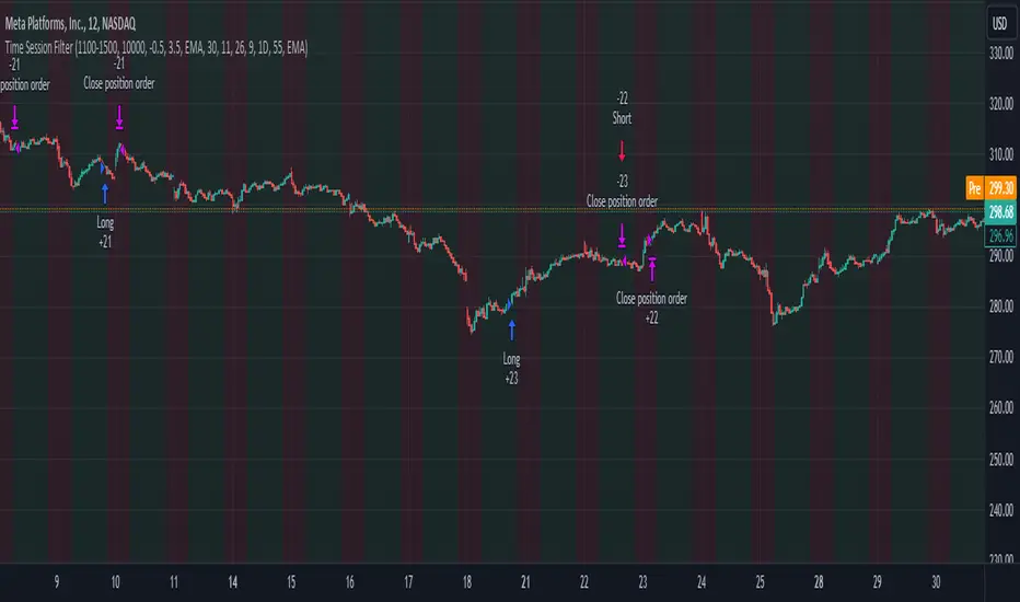
NASDAQ 100 Peak Hours StrategyNASDAQ 100 Peak Hours Trading Strategy
Description
Our NASDAQ 100 Peak Hours Trading Strategy leverages a carefully designed algorithm to trade within specific hours of high market activity, particularly focusing on the first two hours of the trading session from 09:30 AM to 11:30 AM GMT-5. This period is identified for its increased volatility and liquidity, offering numerous trading opportunities.
The strategy incorporates a blend of technical indicators to identify entry and exit points for both long and short positions. These indicators include:
Exponential Moving Averages (EMAs) : A short-term 9-period EMA and a longer-term 21-period EMA to determine the market trend and momentum.
Relative Strength Index (RSI) : A 14-period RSI to gauge the market's momentum.
Average True Range (ATR) : A 14-period ATR to assess market volatility and to set dynamic stop losses and trailing stops.
Volume Weighted Average Price (VWAP) : To identify the market's average price weighted by volume, serving as a benchmark for the trading day.
Our strategy uniquely applies a volatility filter using the ATR, ensuring trades are only executed in conditions that favor our setup. Additionally, we consider the direction of the EMAs to confirm the market's trend before entering trades.
Originality and Usefulness
This strategy stands out by combining these indicators within the NASDAQ 100's peak hours, exploiting the specific market conditions that prevail during these times. The inclusion of a volatility filter and dynamic stop-loss mechanisms based on the ATR provides a robust method for managing risk.
By focusing on the early trading hours, the strategy aims to capture the initial market movements driven by overnight news and the opening rush, often characterized by higher volatility. This approach is particularly useful for traders looking to maximize gains from short-term fluctuations while limiting exposure to longer-term market uncertainty.
Strategy Results
To ensure the strategy's effectiveness and reliability, it has undergone rigorous backtesting over a significant dataset to produce a sample size of more than 100 trades. This testing phase helps in identifying the strategy's potential in various market conditions, its consistency, and its risk-to-reward ratio.
Our backtesting adheres to realistic trading conditions, accounting for slippage and commission to reflect actual trading scenarios accurately. The strategy is designed with a conservative approach to risk management, advising not to risk more than 5-10% of equity on a single trade. The default settings in the script align with these principles, ensuring that users can replicate our tested conditions.
Using the Strategy
The strategy is designed for simplicity and ease of use:
Trade Hours : Focuses on 09:30 AM to 11:30 AM GMT-5, during the NASDAQ 100's peak activity hours.
Entry Conditions : Trades are initiated based on the alignment of EMAs, RSI, VWAP, and the ATR's volatility filter within the designated time frame.
Exit Conditions : Includes dynamic trailing stops based on ATR, a predefined time exit strategy, and a trend reversal exit condition for risk management.
This script is a powerful tool for traders looking to leverage the NASDAQ 100's peak hours, providing a structured approach to navigating the early market hours with a robust set of criteria for making informed trading decisions.
Cari dalam skrip untuk "stop loss"

Time Session Filter - MACD exampleTime Session Filter in TradingView Strategy: A Comprehensive Guide
Welcome to this educational TradingView blog where we dive deep into the functionality and utility of the time session filter in trading strategies. It's interesting to note that the time session filter is a commonly overlooked feature in Pine Script, often not integrated into overall trading strategies. Yet, when used wisely, this tool can significantly enhance your trading approach. In essence, the session filter ensures that trades are only made within a specific, user-defined time frame. By incorporating this often-neglected building block, you can make your strategy more adaptable to various market conditions and trading preferences.
What is a Time Session Filter?
A time session filter is designed to:
Select Times of the Day to Trade: The filter allows you to choose specific hours during the day in which trades are allowed to be excecuted.
Toggle Days to Trade: You can decide which days of the week you want to trade, giving you the flexibility to avoid days that are historically not profitable for your strategy.
Close Trade When Session Ends: The filter can automatically close any open trade once the specified time session concludes, reducing the risk associated with holding positions outside your chosen time frame.
The user interface is streamlined, taking minimal space for the input sections, making it convenient to integrate with other indicators in your overall strategy script. In addition the script colors the background of the chart green when the timesession filter is on and makes the background red when the filter doesn't allow any trades. This helps you to visualise the selected timeframes in relation to chart patterns.
Best Practices for Time Selection
From my personal trading experience I share some input settings you can try to play around with:
Stocks: Trading stocks sometimes yield better results if you only trade in the mornings until lunchtime. This is the period when markets are generally more active, and traders are keenly participating.
Cryptocurrencies: For cryptocurrencies, it sometimes makes sense to avoid trading on Fridays, a day when futures contracts often expire. Various other market-moving events also typically occur on Fridays.
Random Selection: Interestingly, sometimes choosing a random selection of times and days can improve the script's performance, adding an element of unpredictability that might outperform more systematic approaches.
Strategy Overview
This strategy script incorporates various elements, including risk position size and MACD indicator, to provide a comprehensive trading strategy. For a detailed explanation of risk position sizing, please refer to this article:
For a complete understanding of the MACD indicator utilized, visit the following explanation:
Additionally, for high time frame trend filters, consult this resource for more info:
Educational Purposes and Risks
Please note that this script is for educational purposes and serves merely as an example of how to incorporate a time session filter into a trading strategy for pinescript. It is a simplified strategy without a fixed stop-loss, which can result in higher exposure to significant losses. The time session filter can be a powerful addition to your trading strategy, providing you with the tools to tailor your approach according to time-specific market conditions. By understanding its functionalities and best practices, you can make more informed trading decisions, but always remember that trading carries inherent risks.
Happy trading!
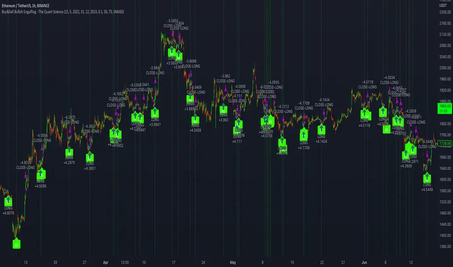
Buy&Sell Bullish Engulfing - The Quant Science🇺🇸
GENERAL OVERVIEW
Buy&Sell Bullish Engulfing - The Quant Science It is a Buy&Sell strategy based on the 'Bullish Engulfing' candlestick pattern. The main goal of the strategy is to achieve a consistent and sustainable return over time, with a manageable level of risk.
Bullish Engulfing
The template was developed at the top of the Indicator provided by TradingView called 'Engulfing - Bullish'.
ENTRY AND EXIT CRITERIA
Entry: A single long order is opened when the candlestick pattern is formed, and the percentage size of the order (%) is fixed by the trader through the user interface.
Exit: The long trade is closed on a percentage equity take profit-stop loss.
----------------------------------------------------------------------------------------------------------------------------------------------------------------------------------------------
🇮🇹
PANORAMICA GENERALE
Buy&Sell Bullish Engulfing - The Quant Science è una strategia Buy&Sell basata sul candlestick pattern 'Bullish Engulfing'. L'obiettivo principale della strategia è ottenere un ritorno costante e sostenibile nel tempo, con un livello gestibile di rischio.
Bullish Engulfing
Il template è stato sviluppato al top dell' Indicatore fornito da Trading View chiamato 'Engulfing - Bullish'.
CRITERI DI ENTRATA E USCITA
Entrata: viene aperto un singolo ordine long quando si forma il candlestick pattern, la size percentuale dell'ordine (%) viene selezionato tramite l'interfaccia utente dal trader.
Uscita: la chiusura della posizione avviene unicamente tramite un take profit-stop loss percentuale calcolato sul capitale.
FRAMA & CPMA Strategy [CSM]The script is an advanced technical analysis tool specifically designed for trading in financial markets, with a particular focus on the BankNifty market. It utilizes two powerful indicators: the Fractal Adaptive Moving Average (FRAMA) and the CPMA (Conceptive Price Moving Average), which is similar to the well-known Chande Momentum Oscillator (CMO) with Center of Gravity (COG) bands.
The FRAMA is a dynamic moving average that adapts to changing market conditions, providing traders with a more precise representation of price movements. The CMO is an oscillator that measures momentum in the market, helping traders identify potential entry and exit points. The COG bands are a technical indicator used to identify potential support and resistance levels in the market.
Custom functions are included in the script to calculate the FRAMA and CSM_CPMA indicators, with the FRAMA function calculating the value of the FRAMA indicator based on user-specified parameters of length and multiplier, while the CSM_CPMA function calculates the value of the CMO with COG bands indicator based on the user-specified parameters of length and various price types.
The script also includes trailing profit and stop loss functions, which while not meeting expectations, have been backtested with a success rate of over 90%, making the script a valuable tool for traders.
Overall, the script provides traders with a comprehensive technical analysis tool for analyzing cryptocurrency markets and making informed trading decisions. Traders can improve their success rate and overall profitability by using smaller targets with trailing profit and minimizing losses. Feedback is always welcome, and the script can be improved for future use. Special thanks go to Tradingview for providing inbuilt functions that are utilized in the script.

SPY 1 Minute Day TraderWhen scalping options, users are looking for where breakouts are going to occur instead of sitting thru areas choppy price action that drain delta and cause them to lose value even if price is up trending. This script tries to identify when a trend reversal is expected based on one minute price action on the SPY. It alerts users to prepare for potential breakout when 5 out of the 6 key optimized parameters are discovered by showing a white L or S. Once all six trigger, it informs the user at the close of that candle with a golden triangle with Pivot Up or Pivot Down. As scalping options is something that is expected to be short in duration, a take profit and stop loss of 30 cents of price actions is established. If five or more parameters occur after the pivot is initiated, then stop losses and take profits are adhered to; however, if there are less, then it waits to take profit or stop the trade, as likely it is just noise and it will finish trend with an additional breakout.
This script has been created to take into account how the following variables impact trend for SPY 1 Minute:
ema vs 13 ema : A cross establishes start of trend
MACD (Line, Signal & Slope) : If you have momentum
ADX : if you are trending
RSI : If the trend has strength
The above has been optimized to determine pivot points in the trend using key values for these 6 indicators
bounce up = ema5 > ema13 and macdLine < .5 and adx > 20 and macdSlope > 0 and signalLine > -.1 and rsiSignal > 40
bounce down = ema5 < ema13 and macdLine > -.5 and adx > 20 and signalLine < 0 and macdSlope < 0 and rsiSignal < 60
White L's indicate that 5 of 6 conditions are met due to impending uptrend w/ missing one in green below it
Yellow L's indicate that 6 of 6 conditions still are met
White S's indicate that 5 of 6 conditions are met due to impending downtrend w/ missing condition in red above it
Yellow S's indicate that 6 of 6 conditions still are met
After a downtrend or uptrend is established, once it closes it can't repeat for 10 minutes
Won't open any trades on last two minutes of any hours to avoid volatility
Will close any open trades going into last minute of hour to avoid large overnight random swings.

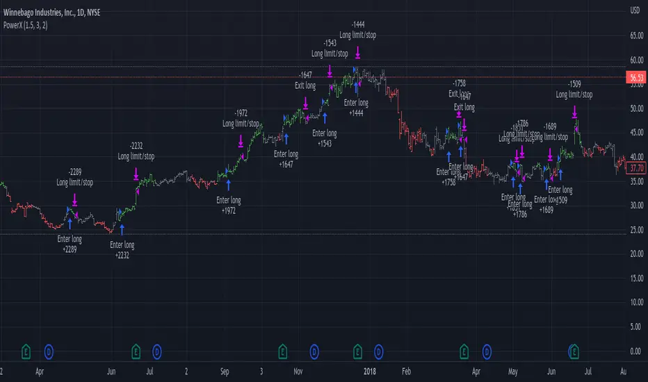
PowerX by jwitt98This strategy attempts to replicate the PowerX strategy as described in the book by by Markus Heitkoetter
Three indicators are used:
RSI (7) - An RSI above 50 indicates and uptrend. An RSI below 50 indicates a downtrend.
Slow Stochastics (14, 3, 3) - A %K above 50 indicates an uptrend. A %K below 50 indicates a downtrend.
MACD (12, 26, 9) - A MACD above the signal line indicates an uptrend. A MACD below the signal line indicates a downtrend
In addition, multiples of ADR (7) is used for setting the stops and profit targets
Setup:
When all 3 indicators are indicating an uptrend, the OHLC bar is green.
When all 3 indicators are indicating a downtrend, the OHLC bar is red.
When one or more indicators are conflicting, the OHLC bar is black
The basic rules are:
When the OHLC bar is green and the preceding bar is black or Red, enter a long stop-limit order .01 above the high of the first green bar
When the OHLC bar is red and the preceding bar is black or green, enter a short stop-limit order .01 below the low of the first red bar
If a red or black bar is encountered while in a long trade, or a green or black bar for a short trade, exit the trade at the close of that bar with a market order.
Stop losses are set by default at a multiple of 1.5 times the ADR.
Profit targets are set by default at a multiple of 3 times the ADR.
Options:
You can adjust the start and end dates for the trading range
You can configure this strategy for long only, short only, or both long and short.
You can adjust the multiples used to set the stop losses and profit targets.
There is an option to use a money management system very similar to the one described in the PowerX book. Some assumptions had to be made for cases where the equity is underwater as those cases are not clearly defined in the book. There is an option to override this behavior and keep the risk at or above the set point (2% by default), rather than further reduce the risk when equity is underwater. Position sizing is limited when using money management so as not to exceed the current strategy equity. The starting risk can be adjusted from the default of 2%.
Final notes: If you find any errors, have any questions, or have suggestions for improvements, please leave your message in the comments.
Happy trading!
Statistical Correlation Algorithm - The Quant ScienceStatistical Correlation Algorithm - The Quant Science™ is a quantitative trading algorithm.
ALGORITHM DESCRIPTION
This algorithm analyses the correlation ratios between two assets. The main asset (on the chart), and the secondary asset (set by the user). Then apply the long or short trading strategy.
The algorithm divides trading work into three parts:
1. Correlation analysis
2. Long or short entry
3. Closing trades
Inside the strategy: the algorithm analyses the percentage change yields from a previous session, of the secondary asset. If the variation meets the set condition then it will open a long or short position, on the primary asset. The open position is closed after 'x' number of sessions. Stop loss and take profit can be added to the trade exit parameters.
Logic: analyses the correlation between two assets and looks for a statistical advantage within the correlation.
INDICATOR DESCRIPTION
The algorithm includes a quantitative indicator. This indicator is used for correlation analysis and offers a quick reading of the quantitative data. The blue area shows the correlation ratio values. The yellow histograms show the percentage change in the yields of the main asset. Purple histograms show the percentage change in secondary asset yields.
GENERAL FEATURES
Multi time-frame: the user can set any time-frame for the secondary asset.
Multi asset: the user analyses the conditions on a second asset.
Multi-strategy: the algorithm can apply either the long strategy or the short strategy.
Built-in alerts: the algorithm contains alerts that can be customized from the user interface.
Integrated indicator: the quantity indicator is included.
Backtesting included: automatic backtesting of the strategy is generated based on the values set.
Auto-trading compliant: functions for auto trading are included.
USER INTERFACE SETTINGS
Through the intuitive user interface, you can manage all the parameters of this algorithm without any programming experience. The user interface is extremely descriptive and contains all the information needed to understand the logic of the algorithm and to configure it correctly.
1. Date range: through this function you can adjust the analysis and working period of the algorithm.
2. Asset: through this function you can adjust the secondary asset and its time-frame. You can enter any type of asset, even indices and economic indicators.
3. Asset details: this function is used to adjust the percentage change to be analyzed on the secondary asset. The analysis and input conditions are also chosen.
4. Active long or short strategy: this function is used to set the type of strategy to be used, long or short.
5. Setting algo trading alert: with this function, users can manage alerts for their web-hook.
6. Exit&Money management: with this function the user can adjust the exit periods of each trade and activate or deactivate any stop losses and take profits.
7. Data Value Analysis: this function is used to adjust the parameters for the quantity indicator.

Booz StrategyBooz Backtesting : Booz Backtesting is a method for analyzing the performance of your current trading strategy . Booz Backtesting aims to help you generate results and evaluate risk and return without risking real capital.
The Booz Backtesting is the Booz Super Swing Indicator equivalent but gives you the ability to backtest data on different charts.
This is an Indicator created for the purpose of identifying trends in Multiple Markets, it is based on Moving Average Crossover and extra features.
Swing Trading: This function allows you to navigate the entire trend until it is not strong enough, so you can compare it with fixed parameters such as Take Profit and Stop Loss.
Take Profit and Stop Loss function: With this function you will be able to choose the most optimal parameters and see in real time the results in order to choose the best combination of parameters.
Leverage : We have this function for the futures markets where you can check which is the most appropriate leverage for your operation.
Trend Filter: allows you to take multiple entries in the same direction of the market.
If the market crosses below the 200 moving average, it will take only short entries.
If the market crosses above the 200 moving average, it will take only long entries.
Timeframes
Charting from 1 Hour, 4 Hour, Daily, Weekly, Weekly
Markets :Booz Backtesting can be tested in Cryptocurrency, Stocks and Futures markets.
Background Color : at a glance, you can see what cycle the market is in.
Green background : Shows that the market is in a bullish cycle.
Red background: Shows that the market is in a bearish cycle.

Bozz Strategy
Booz Backtesting : Booz Backtesting is a method for analyzing the performance of your current trading strategy . Booz Backtesting aims to help you generate results and evaluate risk and return without risking real capital.
The Booz Backtesting is the Booz Super Swing Indicator equivalent but gives you the ability to backtest data on different charts.
This is an Indicator created for the purpose of identifying trends in Multiple Markets, it is based on Moving Average Crossover and extra features.
Swing Trading: This function allows you to navigate the entire trend until it is not strong enough, so you can compare it with fixed parameters such as Take Profit and Stop Loss.
Take Profit and Stop Loss function: With this function you will be able to choose the most optimal parameters and see in real time the results in order to choose the best combination of parameters.
Leverage : We have this function for the futures markets where you can check which is the most appropriate leverage for your operation.
Trend Filter: allows you to take multiple entries in the same direction of the market.
If the market crosses below the 200 moving average, it will take only short entries.
If the market crosses above the 200 moving average, it will take only long entries.
Timeframes
Charting from 1 Hour, 4 Hour, Daily, Weekly, Weekly
Markets :Booz Backtesting can be tested in Cryptocurrency, Stocks and Futures markets.
Background Color : at a glance, you can see what cycle the market is in.
Green background : Shows that the market is in a bullish cycle.
Red background: Shows that the market is in a bearish cycle.
Twitter
Website
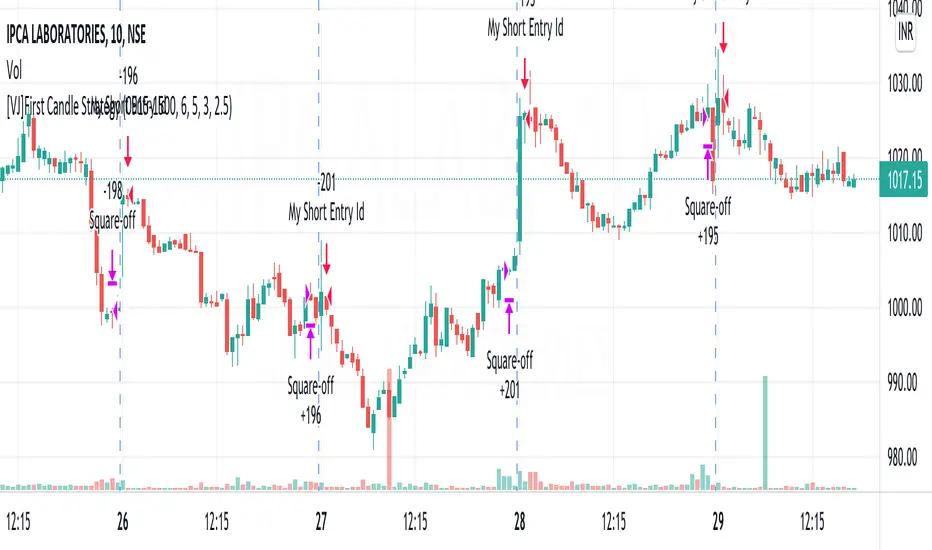
[VJ]First Candle StrategyHello Traders, this is a simple intraday strategy involving the first candle of the day with an additional twist to the traditional style . You can modify the time of candle on the stock and see what are your best picks. Comment below if you found something with good returns
Strategy: Observe the first candle of the day within any time frame. 15m works best. If the first candle is RED ,then go for buy side for the rest of the day. You could square off at close of session or have a fixed take profit and stop loss. This is a contrarian indicator where people just use this as their first entry for the day. The same holds good when a Green candle is seen you go short side.
There is stop loss and take profit that can be used to optimise your trade
The template also includes daily square off based on your time.
Multi Entry Signal Strategy by TradeSmartThis strategy is intended to test different entry signals. You can use 13 different entry signals in the strategy.
Available signals with all their settings:
Heikin Ashi
RSI + EMA
Wavetrend
MACD
Stochastic RSI
Squeeze Momentum
Kairi Relative Index
SSL
Supertrend
Parabolic SAR
Chandelier Exit
Directional Movement Index
Quantitative Qualitative Estimation
For exact rules of entries please relate to the tooltips of each entry signal. All the signals can be used together or separately in the strategy.
Additional settings that can be used:
Trend Filter (limit long or short entries based on a moving average of your choice)
Exit Strategy settings (ATR is used to determine stop loss and take profit levels)
Trailing Loss Setups (you can use 3 different types of trailing losses)
Setups (you can set Long and Short entries as well as the order size based on either Capital % or Risk %)
Date Range (you can limit trades to specific date ranges)
Trading Time (you can limit on which days to trade)
RSI StrategyThis RSI strategy will allow you to go long when RSI is overbought and go short when RSI is oversold. You can also change the checked boxes to reverse this. Uncheck "Overbought Go Long & Oversold Go Short" and check "Overbought Go Short & Oversold Go Long" to use this reversed option.
You can also choose to use an ema filter as an additional qualifier for entry. Uncheck "No EMA Filter" and check "Use EMA Filter" if you want to use it.
Be sure to enter slippage and commission into the properties to give you realistic results.
I've also built in backtesting date ranges and the ability to trade only within certain times of day and have it close all trades at the end of that time frame. This is especially useful for day trading stocks. To specify a time from use the format 0930-1100 or whatever your trading hours will be. Check off "Enable Close Trade At End Of Time Frame" to close the trade at the end of your trading hours.
You can also specify a % based take profit and stop loss. Also keep in mind that the way this code is designed if you use the stop loss and/or take profit and it reaches either target and closes, then it will immediately re-enter if the condition for long or short entry is true.
Finally there's custom alert fields so you can send custom alert messages for strategy entry and exit for use with automated trading services. Simply enter your messages in the fields within the strategy properties and then put {{strategy.order.alert_message}} in your alert message body and it will dynamically pull in the appropriate message.

CCI StrategyThis CCI strategy will allow you to enter a long or short off a CCI zero line cross or control entries and exits from custom upper and lower band lengths. You can set a custom upper band which it will buy when it crosses up and then a custom upper band exit which it will sell when it crosses down. For a short you can set a custom lower band which it will short when it crosses down and the custom lower band exit which it will exit the short when it crosses up. Be sure to enter slippage and commission into the properties to give you realistic results.
I've also built in backtesting date ranges and the ability to trade only within certain times of day and have it close all trades at the end of that time frame. This is especially useful for day trading stocks. If you check off "Enter First Trade ASAP" then when using the time frame option it will enter the current trade. If however you uncheck that box and instead check off "Wait To Enter First Trade" it will wait for the trend to change and then enter.
You can also specify a % based take profit and stop loss. Also keep in mind that if you have "Enter First Trade ASAP" checked off and use the stop loss and/or take profit then it will re-enter the current trend again.
Finally there's custom alert fields so you can send custom alert messages for strategy entry and exit for use with automated trading services. Simply enter your messages in the fields within the strategy properties and then put {{strategy.order.alert_message}} in your alert message body and it will dynamically pull in the appropriate message.

MATIC/USD 1H Bot for 3commas (works w/o 3commas too)This is a MATIC/USD or USDT specific implementation of my BNB/USD 1 hour bot. It should work out of the gate correctly for MATIC, at least based on what has been happening with it for the past seven weeks. You can fiddle with the following settings using the gear icon:
Fast and slow MACD length
The decision to use RSI thresholds as requirements for buys and/or sells, as well as the chart timeframe to use for that (make sure you use the same timeframe as your chart or a higher timeframe. You don't want to use a 1m RSI on a one hour chart but you can use a 4 hour RSI on a 1 hour chart with no issues.)
Buy and/or sell RSI threshold limits
Trailing stop loss %
Start date (for backtesting, I usually leave mine with 1-2 months trailing as those are usually better indicators than how they would have performed over the past few years)
Stress levels
Moving Average length and type
Linear regression amount
The gist of this bot is that it will use a smoothed EMA to make informed buys and sells. The smoothing prevents most noise from affecting your orders. It also allows you to set a trailing stop loss. If you don't want to use this feature set the value to 100 and it will effectively disable it.
Finally, you can disable RSI threshold point visibility. This won't affect bot operation, it just makes it cleaner to look at on your chart. Disabling RSI buys or sells will also disable visibility.
This bot takes a shotgun strategy to buys and sells. It makes a lot of buys and the majority of them are closed with little to no movement up or down. However, the ones that are profitable make a LOT as you will see once you start testing.
I make the full version of these bots available (though the script is protected) so users can test them, however if you want to use it with 3commas you will need access to the full script. Message me if you want the code and we can figure something out.

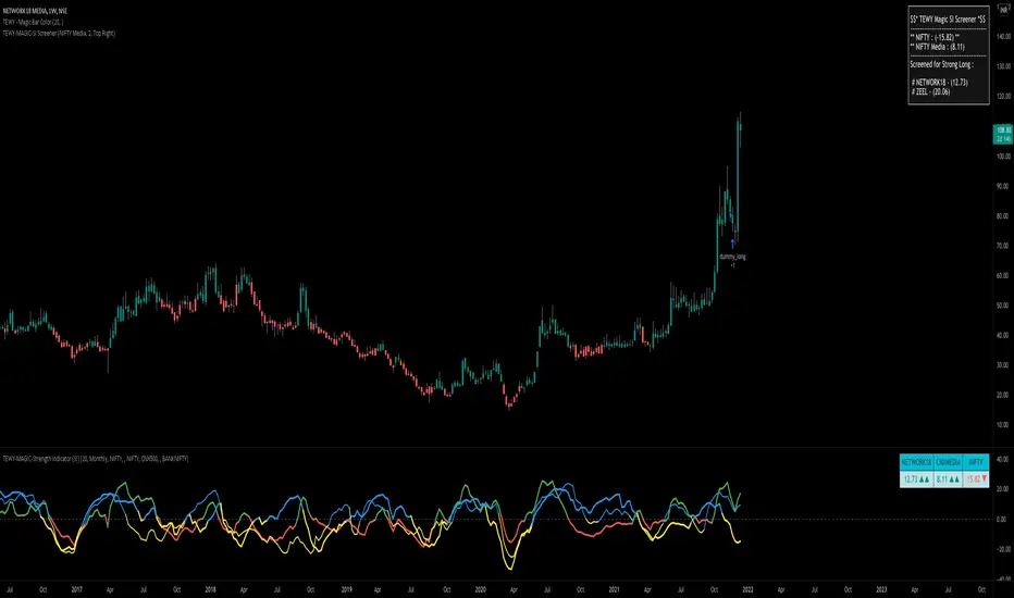
TEWY - Magic Strength Indicator (SI) ScreenerDetail about this indicator
This is screener to identify outperforming Stocks/Ticker based on the indicator "TEWY - Magic Strength Indicator (SI)" I deployed earlier. So please checkout that indicator description to understand more about this screener logic.
Below are the parameters that you may need to use to get outperforming indices/tickers.
1. Screener Set Name :
• Here you can see few of the predefined Index/Ticker sets i created, which you can use to screen Index/Ticker.
• If you select Set for 'Indices' you will get the list of Indices which are out performing NSE:NIFTY. Once you know which index is outperforming, then select the Set for that Index which I already given in the dropdown. That you will get the list of outperforming stock under that index.
• If you want to see all scripts of selected Sector Index that are outperforming NIFTY and may or may not be be outperforming Sector index, then please uncheck the box for "Outperforming Child Index Also". This will get you all the list of Stocks/Tickers which are outperforming Main Index NIFTY.
• If you want to see out-performers for specific period of time then change "How Many Outperforming Candles/Bars" as per your choice
• If you want to see under performers for Short trades then select "Find Short Trades" checkbox
• If you want to see the scripts which are just changed there signal then select "Latest Only" checkbox
Always respect RISKS and follow stop loss. In market stop loss is the only friend of yours.
I have given a sample illustrational image below, which should help you understand this indicator.
Best of luck
DMI (Multi timeframe) DI Strategy [KL]Directional Movement Index Strategy
Entry conditions:
- (a) when DI+ > DI- on timeframe #1, and
- (b) Confirmation: when DI+ > DI- on timeframe #2
In the shown example, timeframe1 was same as the chart (1H) and timeframe2 was 1D.
Stop Loss: ATR based trailing stop
About DMI
Can refer to Investopedia for general understanding.
Applications of DMI in this strategy:
- Assumes uptrend when DI+ is above DI- (when green DI+ lines above red DI-), vice versa for downtrend. This is checked in two different timeframes that can be set by user in settings.
- DX is ignored, it doesn't give a direction of the trend. But if DX was applied, it would be a good indicator for quantifying the strength of uptrend/downtrend. This measurement would typically be read along a threshold (i.e. if below 20, then market is likely consolidating). All of these have been commented out (ignored by pinescript's interpreter via //) in the codes, as said; we are not using DX for sake of simplicity.
Visualizations
To make the chart look cleaner, DMI plots have been simplified to just down/up arrows placed at bottom of the chart.
Referring to the example chart:
- Green arrows : when DI+ > DI- for both timeframes, implies uptrend
- Red arrows: other way around (DI+ < DI-), implies downtrend

Simple EMA Crossing Strategy TradeMathSimple EMA Crossing strategy, based on crossover Fast exponential moving average = EMA21 and Slow exponential moving average = EMA55.
Default stop loss is 3%, but you can change it.
Default take profit is 9%, it based on stop loss.
Risk to Reward ratio is 1 to 3.
Strategy was tested on BTCUSDT 1H timeframe and works fine with these parameters.

LPB MicroCycles StrategyWhat it is:
We use the Hodrick-Prescott filter applied to the closing price, and then take the outputted trendline and apply a custom vwap, the time frame of which is based on user input, not the default 1 day vwap . Then we go long if the value 2 bars ago is greater then one bar ago. We sell and color the bars and lines when the if the value of 2 bars ago is less than one bar ago.
Also included:
GUI for backtesting
ATR Based Stop Loss
How to use:
Go long when the indicators suggest it, and use the stop losses to reduce risk.
Best if paired with a volatility measurement (inside candles, average true range , bollingerband%B)
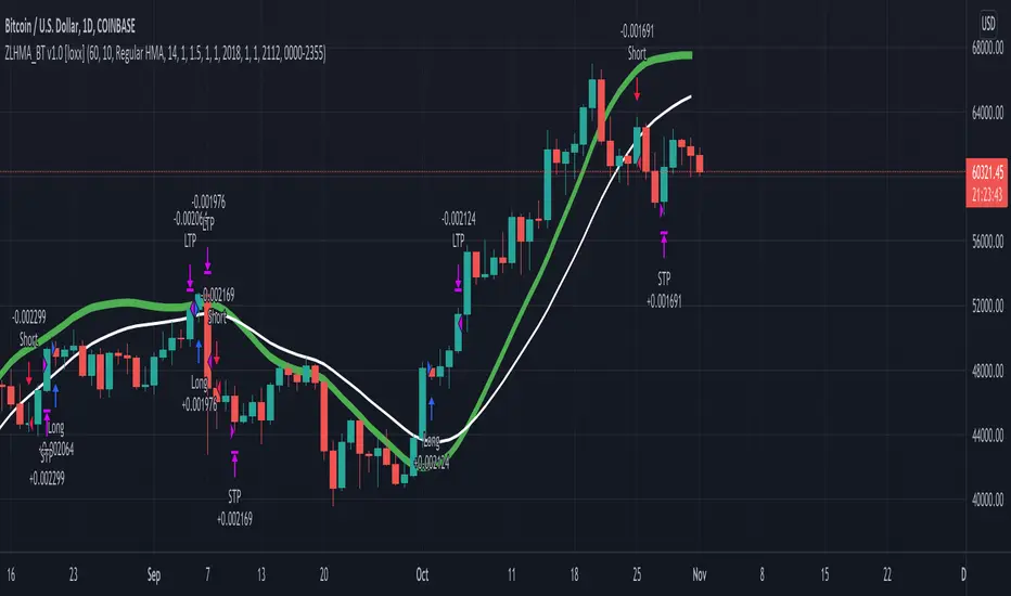
Zero-Lag HMA Backtest v1.0 [loxx]This backtest compares profitability differences between a regular Hull Moving Average ( HMA ) and a Zero-Lag HMA .
Things to know:
- Profit is set to 1 ATR
- Stop-loss is set to 1.5 ATR.
- This is by design to test the minimum the profit scenario (1 ATR up) and the worst case loss scenario (1.5 ATR down) for momentum trading. Actual results vary when additional TPs are added
How to use:
- Adjust settings and dates to view different market structures and position scenarios
- See results in the "Strategy Tester" pane
Conclusions and what's next
- Modifying HMA does very little to improve backtest results
- Future iterations will include options to backtest various moving averages with additional modifiers to improve profits and avoide losses
Comment below or send a PM with questions, comments, observations, or concerns.
BBPBΔ(OBV-PVT)BB - Time Series Decomposition & Volume WeightedThis is an indicator that shows 5 different points of information:
#1 The Trendline is uses a time-series decomposition to remove noise and seasonality data to provide a trendline without using moving averages. This is then further processed by a custom VWAP block that weights it based on the time frame you're currently using.
#2 BB%B - This is the blue histogram that's partially transparent. This is used to find when a security is overbought or oversold.
#3 BB%B of the Δ(OBV-PVT). This is the green histogram. We took the OBV and subtracted the PVT from it, then we found the delta of that compared to the previous candle. This output a line, which we wrapped in bollinger bands to find the BB%B of this line. This line is represented as a histogram, for visual clarity.
#4 Long and Short Indicators: Long is represented by a green dot, and short is represented by a red dot.
#5 Zones - there are multiple zones, which are used to identify overbought and oversold zones.
How to use the indicator:
Simple way: Long on green dot, Short on red dot. Use stop losses and take profits.
Slightly More Complex: Same as above, but also close out longs, when the green histogram drops but the blue does not. As this means price action hasn't caught up with volume. Use stop losses and take profits.
Full Usage: Long only when both the green, blue and yellow lines are below 0, and sell when the blue or green histogram rises above 1. Perform the opposite for the shorting. Ignore the dots if you use this method, they are for simple reference points til you get used to this indicator. Use stop losses and take profits.

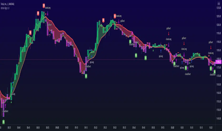
vStrat Algo 1.0 (BETA)vStrat Algo 1.0
The Very First Scalping/Intraday Trading Algo for Options
Note: If you have any favorite indicators that you use regularly and are helpful, feel free to use them in conjunction to this strategy.
Legend:
long = buy call
short = buy put
close entry = sell call/put
BULL = bullish engulfing
BEAR = bearish engulfing
OS = oversold
OB = overbought
Instructions:
1. You can choose to watch the 3 minute or 5 minute chart but be aware of the Pro’s and Con’s. It’s not recommended to use this strategy on the 1 minute chart, but this works on higher timeframes. Keep in mind that the signals will vary on each timeframe.
3 minute 5 minute
i.ibb.co i.ibb.co
2. It’s best to use this strategy right at market open. If a “long” (buy CALLS) or “short” (buy PUTS) signal was given at pre-market, I do not recommend taking it. Only take signals once the market opens. If you really wish to take the signal that was given 1-5 minutes before the market opened, you most definitely can, but its’s just riskier. What I would do is, wait 3-10 minutes after market open and if one Moving Average is respecting the other and holding above or below it, you can enter especially if the blow is bullish, the vStrat Algo 1.0 will also tell you if the candles are bearish or bullish. Use your best judgement.
i.ibb.co [
3. You do not have to wait for the exit signal, everyone's risk management is different so take profits whenever you're green or hold as long as the short-term MA is still trending above or below the long-term MA and is not touching or bouncing off it.
i.ibb.co
4. Avoid taking any signals from 11:30 AM ET - 2:30 PM ET, when stocks are trading sideways since the algo’s stop losses get triggered here due to the low volume.
i.ibb.co
5. Lastly, there is no magic indicator or strategy, this algorithm is designed based on multiple conditions. Each signal gets triggered when ALL the conditions are met. This strategy is based off advanced moving averages, one that reduces lag and responds quicker than the simple and exponential ones, RSI value, S/R, pivot points, and a few others. I’m always looking for ways to improve this scalping algorithm so rest assured any complaints or suggestions will be taken and fixed as timely as possible. For best results, avoid trading with your emotions. If you’re a new user, open a small position, set a stop loss, and let the algorithm decide how you will trade it for that day. Keep doing this until you get more familiar with the script then slowly increase your position sizing, but do not invest money you can’t afford to lose. Play with the settings, change the lengths if you wish, but the script was created to provide the most accurate signals as it is. If you do decide to change these inputs, the signals will also be different. Take profits whenever you see fit, the goal is to have a green day and grow your account slowly but surely. If you make a profit, do not risk giving your money back to the market by overtrading. Always do your own due diligence and use your best judgement. Good luck, Traders!
DISCLAIMER : All information found here, including any ideas, opinions, views, predictions, forecasts, commentaries, suggestions, or stock picks, expressed, or implied herein, are for informational, entertainment or educational purposes only and should not be construed as personal investment advice. While the information provided is believed to be accurate, it may include errors or inaccuracies. Conduct your own due diligence or consult a licensed financial advisor or broker before making any and all investment decisions. Any investments, trades, speculations, or decisions made on the basis of any information found on this site, expressed, or implied herein, are committed at your own risk, financial or otherwise.
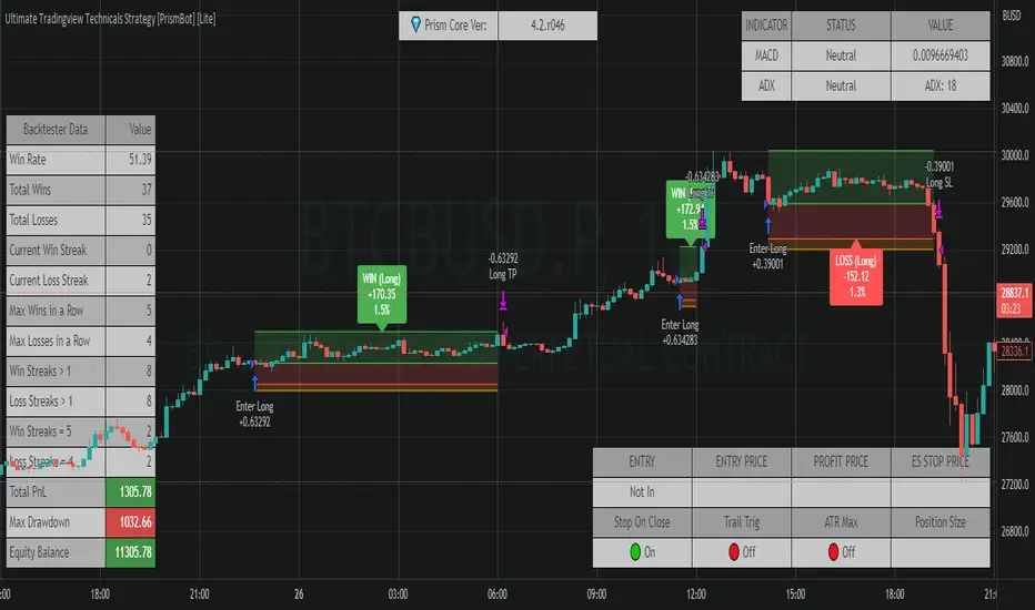
Ultimate Tradingview Technicals Strategy [PrismBot] [Lite]Included in this builder:
MACD
RSI
Tradingview Technical Analysis
Ichimoku
Global Trend Filter
Pullback Filter
Our most robust strategy to date with MACD , RSI , and many other basic strategies included as well as additional filters and alert options.
It is an advanced trading strategy built with the intent to make it easy for anyone to begin trading, but also avoid too much complication of strategy concepts.
For instance, you can change the MACD settings to be "more sensitive" by using a simple dropdown menu, and adjust which strategy you are employing with the MACD on the fly with another.
You can easily enable and disable strategies using the checkbox.
The strategy demo results use 100% equity per trade as an example - the reason for this is that the stop loss is set to 1%, so each trade is risking 1% (give or take slippage). Slippage is set to 5 ticks, and a 0.04% commission (Binance average for market and limit orders)
This strategy incorporates a risk to reward system where the user can select between ATR and Percent based stop losses and take profit targets. This means that the user has much better control over money management when utilizing this strategy and it doesn't require you to babysit the strategy to ensure it's entering and existing strategies in an ideal place.
The status box shows the current state of the various strategies and their values. A red circle indicates the filter / strategy is not valid for entry yet. A green circle indicates that filter / strategy is valid for entry. When all selected strategies are valid simultaneously, the next bar will trigger an entry signal.
If you have any questions about this strategy, please leave them in the comments below, or DM for more details. Thanks!
Additional features in this lite strategy:
✔️ Tweak a multitude of specific settings (MA lengths, R:R, SL distance etc)
✔️ Use money management and risk calculations
✔️ Draw trade info directly to chart (eg. SL size in percent, win rate etc)
✔️ Use various filters (eg. time filter, date filter etc)
✔️ Manage risk per position
✔️ Sync to any bot or algorithmic trading system
SSP + VWMAInput menu allows you to set long / short entries using,
Net volume change from above or below zero.,
Net volume changes of positive to negative values,
VWAP rising or falling.
VWMA rising or falling
Stop loss and take profit are built in to test the most profitable strategy.
uncheck net volume in menu bar to remove background colours on chart
Uncheck VWAP and VWMAto test long and short entries ( using net volume change ) note session look back is available to edit, if use take profit is unchecked then this will simulate net volume change from positive to negative.
Check VWMA or VWAP to simulate long or short entries
With VWAP checked this will simulate VWAP entries with rising / falling VWAP with previous take profit and stop losses that we’re profitable.
