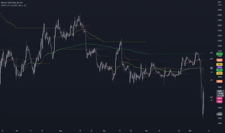
VWAP & Previous VWAP - MTF█ Volume Weighted Average Price & Previous Volume Weighted Average Price - Multi Timeframe
This script can display the daily, weekly, monthly, quarterly, yearly and rolling VWAP but also the previous ones.
█ Volume Weighted Average Price (VWAP)
The VWAP is a technical analysis tool used to measure the average price weighted by volume.
VWAP is typically used with intraday charts as a way to determine the general direction of intraday prices.
VWAP is similar to a moving average in that when price is above VWAP, prices are rising and when price is below VWAP, prices are falling.
VWAP is primarily used by technical analysts to identify market trends.
█ Rolling VWAP
The typical VWAP is designed to be used on intraday charts, as it resets at the beginning of the day.
Such VWAPs cannot be used on daily, weekly or monthly charts. Instead, this rolling VWAP uses a time period that automatically adjusts to the chart's timeframe.
You can thus use the rolling VWAP on any chart that includes volume information in its data feed.
Because the rolling VWAP uses a moving window, it does not exhibit the jumpiness of VWAP plots that reset.
For the version with standard deviation bands.
MTF VWAP & StDev Bands
Cari dalam skrip untuk "weekly"
Nasy -- Daily, Weekly, Monthly MADaily High Low, Daily Open Close, Weekly High Low, Weekly Open Close, Monthly High Low, Monthly Open Close

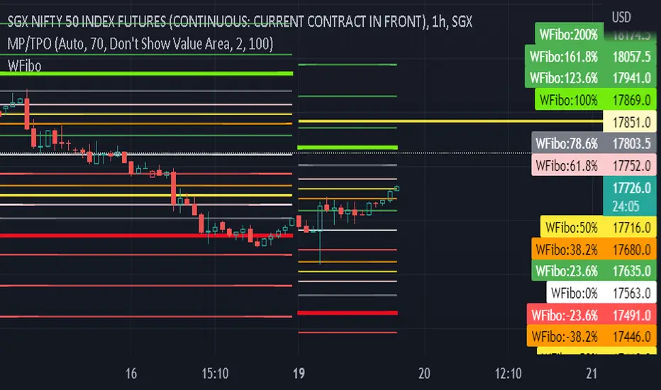
Fibonacci Ratios with Volatility(Weekly Time Frame.)Script is based on weekly time Frame. Fib ratios are drawn at the Open of the Market. Open price is compared with Previous week High , low and close. If weekly open is above Previous week high or low, Fib 0 % is plotted above High or the low as the case may be . If weekly open is between previous week high and low Fib 0% is equal to previous week Close and other fib ratios are plotted accordingly. As its vol based, works fantastically. This script is inspired by Fibonacci and Volatility script by PB GHOSH.
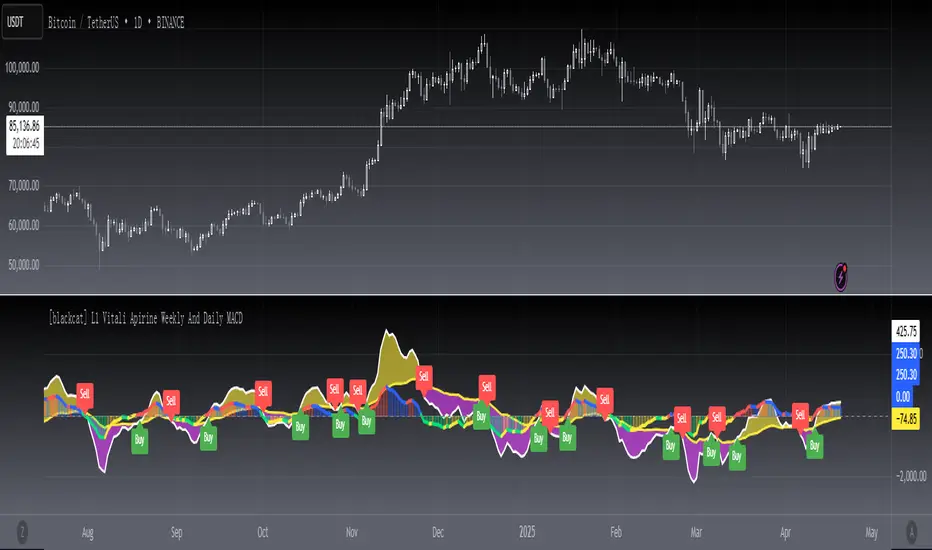
[blackcat] L1 Vitali Apirine Weekly And Daily MACDLevel 1
Background
This indicator was originally formulated by Vitali Apirine for TASC - December 2017 Traders Tips, “Weekly & Daily MACD”.
Function
In the article “Weekly & Daily MACD” in this issue, author Vitali Apirine introduces a novel approach to using the classic MACD indicator in a way that simulates calculations based on different timeframes while using just a daily-interval chart. He describes a number of ways to use this new indicator that allows traders to adapt it to differing markets and conditions.
Remarks
Feedbacks are appreciated.
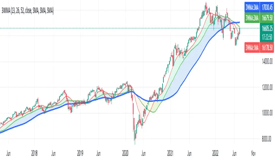
Triple Weekly Moving AverageTriple Weekly Moving Average
The default settings plot 3 weekly moving averages for 13, 26 and 52 weeks, for analyzing Short (Quarterly), Medium (Semester) and long term (Yearly) view.
Idea is when the three moving averages are aligned, the security is in trend and when they crisscross the security may be either turning, slowing down or stalling, however, this must be correlated with other studies.
Started observing half yearly moving average after reading Stan Weinstein's Secrets For Profiting in Bull and Bear Markets .
The settings of the indicator are pretty self explanatory. The indicator gives an option to select lookahead , however, change it only when you are well aware of the consequences, the default setting is Turned Off , please follow TV user guide for a detailed explanation on lookahead. I added it as I was plotting this script on Daily timeframe and wanted to observe the changes.
[blackcat] L2 Vitali Apirine Weekly & Daily StochasticsLevel 2
Background
Vitali Apirine’s articles in the Sep issues on 2018,“Weekly & Daily Stochastics”
Function
In “Weekly & Daily Stochastics” in this issue, author Vitali Apirine introduces a novel approach to using the classic stochastic indicator in a way that simulates calculations based on different timeframes while using just a daily interval chart. He describes a number of ways to use this new indicator that allows traders to detect the state of longer-term trends while looking for entry points and reversals. Here, I am providing the TradingView pine code for an indicator based on the author’s ideas.
Remarks
Feedbacks are appreciated.

Waddah Attar Weekly Camarilla Pivots [Loxx]Waddah Attar Weekly Camarilla Pivots is an indicator built by Ahmad Waddah Attar that draws weekly Camarilla over lower timeframes.
What are Camarilla pivots?
Camarilla Pivot Points is a math-based price action analysis tool that generates potential intraday support and resistance levels. Similar to classic pivot points, it uses the previous day's high price, low price, and closing price.
Camarilla Pivot Points is a modified version of the classic Pivot Point. Camarilla Pivot Points were introduced in 1989 by Nick Scott, a successful bond trader. The basic idea behind Camarilla Pivot Points is that price has a tendency to revert to its mean until it doesn’t. What makes it different than the classic pivot point formula is the use of Fibonacci numbers in its calculation of pivot levels. Camarilla Pivot Points is a math-based price action analysis tool that generates potential intraday support and resistance levels.
Details
-Used for intraday trading to identify support/resistance levels
-Restricted to timeframes 4 hours and below
-Unlike most versions of Weekly Camarilla Pivots, this version allows you to customize the Fibonacci levels

DKNS_Daily Weekly Monthly High Low Open CloseDKNS_Daily Weekly Monthly High Low Open Close, it will give daily weekly monthly high low close open

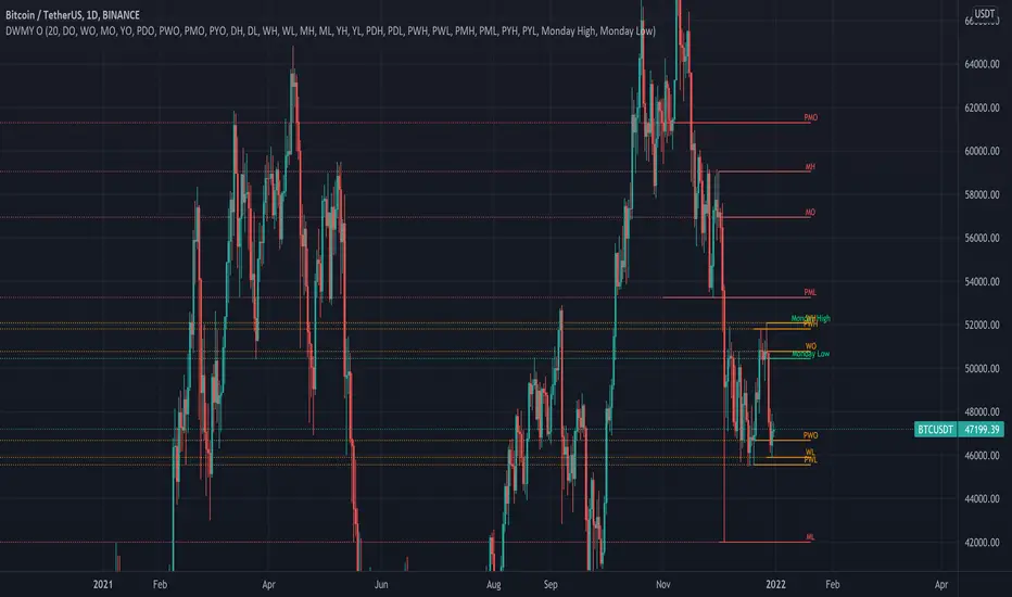
Daily Weekly Monthly Yearly OpensThis indicator draws key level lines such as daily open, weekly open, monthly open, yearly open, previous daily open, previous weekly open, previous monthly open, previous yearly open, monday daily high and monday daily low to chart. This lines can act either support or resistance but it is just possibility. This lines will help you to find buy and sell places.
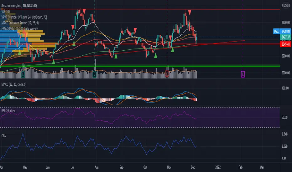
EMA 20/50/100/200 Daily-WeeklyHello!
In case this helps others when using EMA's on multiple timeframes, I decided to publish this script I modified.
It adds the EMA for 20/50/100/200 timeframes and gives them the color white, orange, red, green respectively.
The weekly timeframe will get the corresponding weekly EMA.
The monthly timeframe will get the corresponding monthly EMA.
The daily timeframe, and all timeframes below this, will get the daily timeframe. The idea that that a ticker symbol might respect with strength the daily EMA's - you'll be able to move to a smaller timeframe and still view the daily EMA's in an effort to better view how close the ticker came to taking a specific EMA.
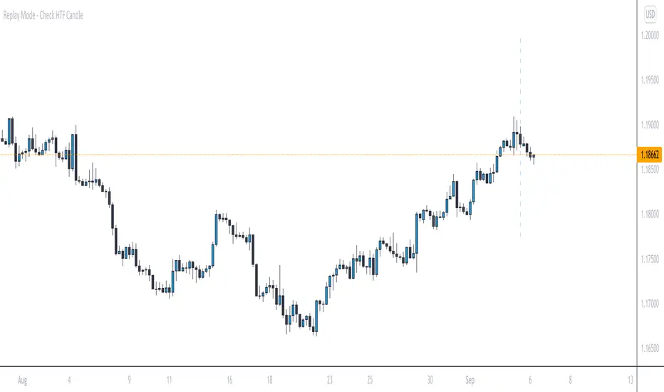
Replay Mode - Check HTF CandleThis indicator is intended to be used while using Replay Mode.
A vertical line will be drawn when you can safely check the 4H, Daily, or Weekly candle without seeing future price.
It is similar to the built-in Session Breaks, but has the benefit of not needing to remove one candle before checking the Daily.
When the line is the color of your 4H settings, it is safe to check the 4H candle.
When the line is the color of your Daily settings, it is safe to check the 4H and Daily candles.
When the line is the color of your Weekly settings, it is safe to check the 4H, Daily and Weekly candles
First Week Trend [MX]I created this indicator based on one of my ways of analyzing the BTC trend in particular, I noticed that the break of the first weekly candle usually indicates the trend for the rest of the month.
This indicator has a bug in which if you change the timeframe of the indicator it will show erroneous values
If you use the candlestick chart, you will need to pull the visual order of this indicator to the top to overlay the colors of the standard candles, or simply hide the standard candles
the trend colors are bugged in timeframes other than the weekly
special thanks to @xdecow who helped me with the code
////////////////////////////////////////////////////////////////////////
Eu criei esse indicador baseado em uma das minhas formas de analisar a tendência do BTC em específico, eu notei que o rompimento do primeiro candle do semanal costuma indicar a tendência para o resto do mês.
Esse script tem um bug em que se mudar o timeframe do indicador ele irá mostrar valores errados
Se você usa o gráfico de candlesticks, você precisará puxar para o topo a ordem visual desse indicador para sobrepor as cores do candles padrões, ou simplesmente ocultar os candles padrões
as cores da tendencia estão bugados em outros timeframes diferentes do semanal
agradecimentos especiais ao @xdecow que me ajudou no código

Pre and Market OpeningsPre and Market Openings is to enable you to quickly visualize the opening markets and how they could influence trading.
The below script has used the market time data from the below links:
Tokyo/Asia www.tradinghours.com
London www.tradinghours.com
New York www.tradinghours.com
The below script aims to plot:
Daily Asia Open
Weekly Asia Open
Daily London Open
Weekly London Open
Daily New York Open
Weekly New York Open
Using background colour it also shows market sessions (pre-market) for London and New York and regular for London, New York and Asia.
There is also plotted text for days of the week and sessions.
As you can see from the picture below that these market openings can act as support and resistance:
BTC
ETH

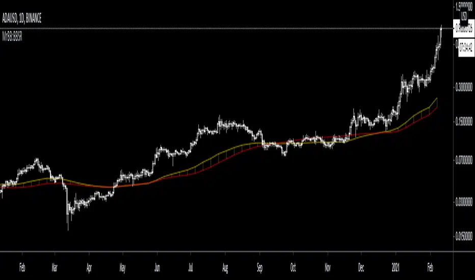
MrBB:BullBear Support BandVery simple and effective S/R band. Created bycombining the weekly 21EMA and weekly 20SMA, it provides strong support/resistance depending on market direction, and works as a basing area for retraces during parabolic (and normal) bull markets.
Fibonacci Pivots Monthly and Weekly Full (no history)Fibonacci Pivots Monthly and Weekly Full (no history)
Inspired by FxChartAnalyst trader, with his great Monthly Weekly Daily Pivot Points Standard indicator
www.tradingview.com
This indicator calculates and plots both Monthly and Weekly pivots on a chart. Pivots are based on the Fibonacci ratios of the previous Month/Week candle close.
Good luck everyone!

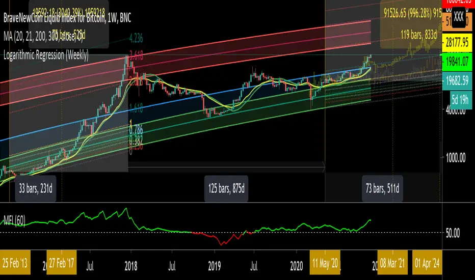
Logarithmic Regression (Weekly)This script is a combination of different logarithmic regression fits on weekly BTC data. It is meant to be used only on the weekly timeframe and on the BLX chart for bitcoin. The "fair value" line is still subjective, as it is only a regression and does not take into account other metrics.
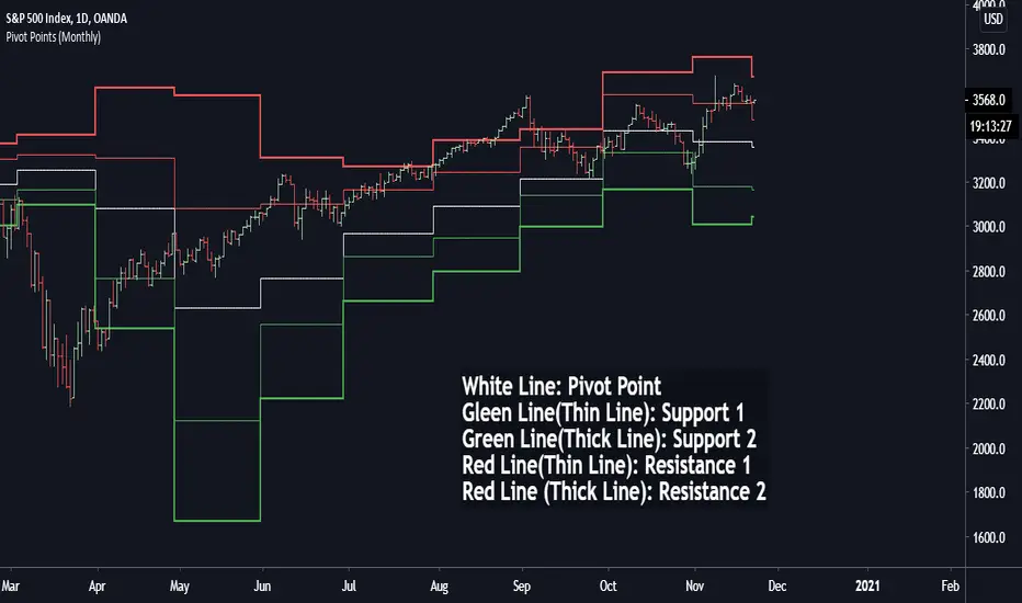
Pivot Points (Daily, Weekly, Monthly)Pivot point: P = (High + Low)/2
First support: S1 = Low
Second support, S2 = Low - 2 * (High - Low)
First resistance: R1 = High
Second resistance, R2 = High + 2 * (High - Low)
White Line: Pivot Point
Gleen Line(Thin Line): Support 1
Green Line(Thick Line): Support 2
Red Line(Thin Line): Resistance 1
Red Line (Thick Line): Resistance 2
You can adjust it to daily, weekly or monthly indicators, daily for intraday trading (1minute, 1hour etc.), weekly and monthly for day/swing trading, monthly for weekly trades. I plot the graph with steplines since I think they can show the differences of pivots from time to time more clearly, you are free to change to other plot styles like circles or regular lines if you want to. Please like this script, and let me know any questions, thanks.
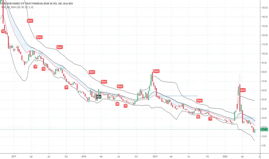
Short in Bollinger Band Down trend (Weekly and Daily) // © PlanTradePlanMM
// 6/14/2020
// ---------------------------------------------------
// Name: Short in Bollinger Band Down trend (Weekly and Daily)
// ---------------------------------------------------
// Key Points in this study:
// 1. Short in BB Lower band, probability of price going down is more than 50%
// 2. Short at the top 1/4 of Lower band (EMA - Lower line), Stop is EMA, tartget is Lower line; it matches risk:/reward=1:3 naturally
//
// Draw Lines:
// BB Lower : is the Target (Black line)
// BB EMA : is the initial Stop (Black line)
// ShortLine : EMA - 1/4 of (Stop-target), which matches risk:/reward=1:3
// Prepare Zone : between EMA and ShortLine
// shortPrice : Blue dot line only showing when has Short position, Which shows entry price.
// StopPrice : Black dot line only showing when has Short position, Which shows updated stop price.
//
// Add SMA50 to filter the trend. Price <= SMA, allow to short
//
// What (Condition): in BB down trend band
// When (Price action): Price cross below ShortLine;
// How (Trading Plan): Short at ShortLine;
// Initial Stop is EMA;
// Initial Target is BB Lower Line;
// FollowUp: if price moves down first, and EMA is below Short Price. Move stop to EMA, At least "make even" in this trade;
// if Price touched Short Line again and goes down, new EMA will be the updated stop
//
// Exit: 1. Initial stop -- "Stop" when down first, Close above stop
// 2. Target reached -- "TR" when down quickly, Target reached
// 3. make even -- "ME" when small down and up, Exit at Entry Price
// 4. Small Winner -- "SM" when EMA below Entry price, Exit when Close above EMA
//
// --------------
// Because there are too many flags in up trend study already, I created this down trend script separately.
// Uptrend study is good for SPY, QQQ, and strong stocks.
// Downtrend Study is good for weak ETF, stock, and (-2x, -3x) ETFs, such as FAZ, UVXY, USO, XOP, AAL, CCL
// -----------------------------------------------------------------------------------------------------------------
// Back test Weekly and daily chart for SPY, QQQ, XOP, AAL, BA, MMM, FAZ, UVXY
// The best sample is FAZ Weekly chart.
// When SPY and QQQ are good in long term up trend, these (-2x, -3x) ETFs are always going down in long term.
// Some of them are not allowed to short. I used option Put/Put spread for the short entry.
//
Buy in Bollinger Band uptrend (Weekly and Daily) // © PlanTradePlanMM 6/14/2020
// ---------------------------------------------------
// Name: Buy in Bollinger Band uptrend (Weekly and Daily)
// ---------------------------------------------------
// Key Points in this study:
// 1. Long in BB Upper band, probability of price going up is more than 50%
// 2. Buy at the bottom 1/4 of upper band (Upper line - EMA), Stop is EMA, tartget is Upper line; it matches risk:reward=1:3;
//
// Draw Lines:
// BB Upper : is the Target (Black line)
// BB EMA : is the initial Stop (Black line)
// BuyLine : EMA20 + 1/4 of (Target-Stop), which matches risk:/reward=1:3 naturally
// Prepare Zone : between EMA and BuyLine
// buyPrice : Blue dot line only showing when has long position, Which shows entry price.
// StopPrice : Black dot line only showing when has long position, Which shows updated stop price.
//
// Add SMA(50) to filter the trend. Price >= SMA, allow to long
//
// What (Condition): in BB uptrend band
// When (Price action): Price cross over BuyLine;
// How (Trading Plan): Buy at BuyLine;
// Initial Stop is EMA;
// Initial Target is BB Upper Line;
//
// FollowUp: if price moves up first, and the EMA is higher than Entry point, Use EMA as new stop. At least "make even" in this trade;
//
// Exit: 1. Initial stop -- "Stop" when down first, close below stop price.
// 2. Target reached -- "TR" when up quickly, Target reached
// 3. make even -- "ME" when small up and down, Exit at entry Price
// 4. Small Winner -- "SM" when EMA above Entry price, Exit when close below EMA, and higher than entry Price
//
// --------------
// Because there are too many flags in up trend study already, I will create a down trend script separately.
// Uptrend study is good for SPY, QQQ, and strong stocks.
// Downtrend Study is good for weak ETF, stock, and (-2x, -3x) ETFs, such as FAZ, UVXY, USO, XOP, AAL, CCL
// -----------------------------------------------------------------------------------------------------------------
// Back test Weekly and daily chart for SPY, QQQ
// If it will be a big Gap down or a big down move, stop at close price could be a big loss; But this way could avoid may noise, to stay in a trending position longer.
// When buy in trending move, the position could be hold for a big range.
// The best samples are SPY and QQQ daily chart.
//
// Better to use another way to verify the long term up trend first.
// For single stock, it is better shows more relative strength than SPY.

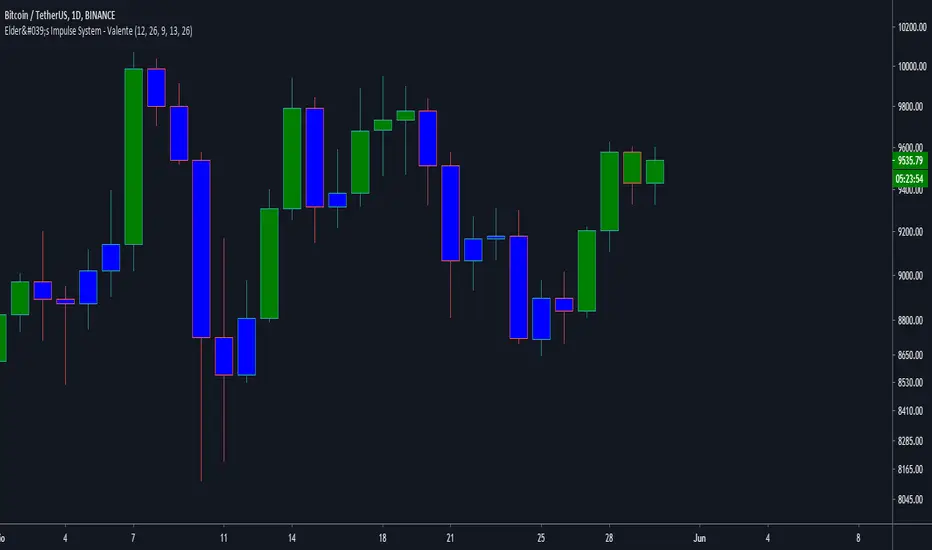
Elder's Impulse System with weekly EMA Filter - ValenteThis indicator was based on the Elders Impulse System by astraloverflow.
The only difference is that I included the weekly EMA26 as a filter and you can plot it on the graph if you want (unchecking the Weekly EMA26 won't turn the filter off, will only stop plotting it).
The indicator works this way:
When the MACD Histogram is growing UP, the EMA13 is pointing UP AND the Weekly EMA26 is pointing UP, the bar is Green
When the opposite is true, the bar is Red.
When any condition from both green and red is not true, the bar is blue.
In my opinion, this particular indicator works better on the D1 time frame. I recommended using the original one, by astraloverflow for other time frames.
I hope it is useful!
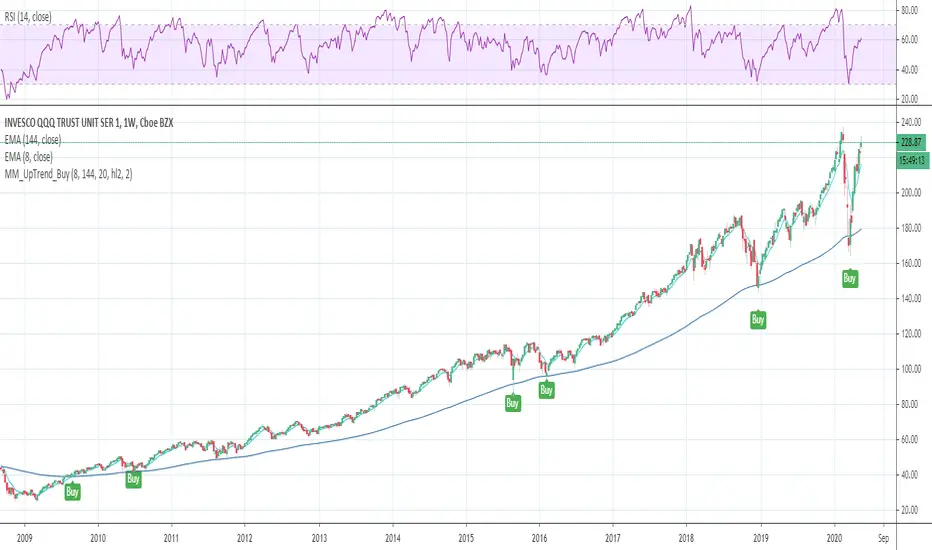
Buy in long term uptrend (Weekly and Daily)Condition: in uptrend, EMA8 > EMA144 (User can change the EMA# from input);
Price Action: (Price crossover EMA144) or (price touched EMA144 and close above it);
Trading Plan: Buy at close or next open; Initial Stop below EMA144;
No Exit strategy in this study, trader needs to move stop by other rules; such as, uptrend line break;
Back test Weekly and daily chart for SPY, QQQ, TLT, GLD, IWM, XLF, XLK, XOP, GS, IBM, APPL, CAT, LVS
1. When side way move or price From uptrend to Down trend, Entry could be stopped quickly with small loss;
2. When buy in trending move, the position could be hold for few years.
The best sample is QQQ weekly chart.
This is my first tradingview script. I created this script file and tested in one week.
Maybe, this script is too simple, other people published similar code already; Sorry, I didn't Check that yet.
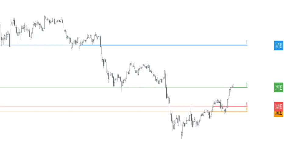
Daily Weekly Monthly Yearly OpensThis script plots the current daily, weekly and monthly opens (all enabled by default).
Here are some additional info about the drawing behavior:
Daily open is shown only on intraday timeframes
Weekly open is shown only on timeframes < weekly
Monthly open is shown only on timeframes < monthly
High/Low Weekly TimeframeI'm testing a simple but useful indicator that plots the high and low for the current week. The time-frame can be selected by the user.
It's useful when you're trading in a smaller time-frame (example: 1H or 4H) to know exactly the weekly low and high, and whether the price breaks above or below this price lines.
This indicator allows you:
- To select the desired time-frame to get the Low and High.
- To print an optional EMA for the same time-frame.
- To optionally change the bar-color when the close price crosses above the weekly high or crosses below the weekly low.
Hope this helps you to visually identify price movements.
If you like this script please give me a like and comment below.
Thanks,
Rodrigo