Order Block Matrix [Alpha Extract]The Order Block Matrix indicator identifies and visualizes key supply and demand zones on your chart, helping traders recognize potential reversal points and high-probability trading setups.
This tool helps traders:
Visualize key order blocks with volume profile histograms showing liquidity distribution.
Identify high-volume price levels where institutional activity occurs.
rank historical order blocks and analyze their strength based on volume.
Receive alerts for potential trading opportunities based on price-block interactions.
🔶 CALCULATION
The indicator processes chart data to identify and analyze order blocks:
Order Block Detection
Inputs:
Price action patterns (consolidation areas followed by breakouts).
Volume data from current and lower timeframes.
User-defined lookback periods and thresholds.
Detection Logic:
Identifies consolidation areas using a dynamic range comparison.
Confirms breakout patterns with percentage threshold validation.
Maps volume distribution across price levels within each order block.
🔶Volume Analysis
Volume Profiling:
Divides each order block into configurable grid segments.
Maps volume distribution across price segments within blocks.
Highlights zones with highest volume concentration.
Strength Assessment:
Calculates total block volume and relative strength metrics.
Compares block volume to historical averages.
Determines probability of reversal based on volume patterns.
isConsolidation(len) =>
high_range = ta.highest(high, len) - ta.lowest(high, len)
low_range = ta.highest(low, len) - ta.lowest(low, len)
avg_range = (high_range + low_range) / 2
current_range = high - low
current_range <= avg_range * (1 + obThreshold)
🔶 DETAILS
Visual Features
Volume Profile Histograms:
Color-coded bars showing volume concentration within order blocks.
Gradient coloring based on relative volume (high volume = brighter colors).
Bull blocks (green/teal) and bear blocks (red) with varying opacity.
Block Visualization:
Dynamic box sizing based on volume concentration.
Optional block borders and background fills.
Volume labels showing total block volume.
Screener Table:
Real-time analysis of order block metrics.
Shows block direction, proximity, retest count, and volume metrics.
Color-coded for quick reference.
Interpretation
High Volume Areas: Zones with institutional interest and potential reversal points.
Block Direction: Bullish blocks typically support price, bearish blocks typically resist price.
Retests: Multiple tests of an order block may strengthen or weaken its influence.
Block Age: Newer blocks often have stronger influence than older ones.
Volume Concentration: Brightest segments within blocks represent the highest volume areas.
🔶 EXAMPLES
The indicator helps identify key trading opportunities:
Bullish Order Blocks
Support Zones: Identify strong support levels where price is likely to bounce.
Breakout Confirmation: Validate breakouts with volume analysis to avoid false moves.
Retest Strategies: Enter trades when price retests a bullish order block with high volume.
Bearish Order Blocks
Resistance Zones: Identify strong resistance levels where price is likely to reverse.
Distribution Areas: Detect zones where smart money is distributing to retail.
Short Opportunities: Find optimal short entry points at high-volume bearish blocks.
Combined Strategies
Order Block Stacking: Multiple aligned blocks create stronger support/resistance zones.
Block Mitigation: When price breaks through a block, it often indicates a strong trend continuation.
Volume Profile Applications: Higher volume segments provide more precise entry and exit points.
🔶 SETTINGS
Customization Options
Order Block Detection:
Consolidation Lookback: Adjust the period for consolidation detection.
Breakout Threshold: Set minimum percentage for breakout confirmation.
Historical Lookback Limit: Control how far back to scan for historical order blocks.
Maximum Order Blocks: Limit the number of visible blocks on the chart.
Visual Style:
Grid Segments: Adjust the number of volume profile segments.
Extend Blocks to Right: Enable/disable extending blocks to current price.
Show Block Borders: Toggle border visibility.
Border Width: Adjust thickness of block borders.
Show Volume Text: Enable/disable volume labels.
Volume Text Position: Control placement of volume labels.
Color Settings:
Bullish High/Low Volume Colors: Customize appearance of bullish blocks.
Bearish High/Low Volume Colors: Customize appearance of bearish blocks.
Border Color: Set color for block outlines.
Background Fill: Adjust color and transparency of block backgrounds.
Volume Text Color: Customize label appearance.
Screener Table:
Show Screener Table: Toggle table visibility.
Table Position: Select positioning on the chart.
Table Size: Adjust display size.
The Order Block Matrix indicator provides traders with powerful insights into market structure, helping to identify key levels where smart money is active and where high-probability trading opportunities may exist.
Cari dalam skrip untuk "zone"

TLC sessionA Professional Intraday Session Tracker with VWAP and Economic Event Integration
Description
This indicator provides visual tracking of major trading sessions (Asian, London, New York) combined with VWAP calculations and macroeconomic event zones. It's designed for intraday traders who need to monitor session overlaps, liquidity periods, and high-impact news events.
The basic script of trading sessions was taken as a basis and refined for greater convenience.
Key Features:
Customizable Session Tracking: Visualize up to 3 trading sessions with adjustable time zones (supports IANA & GMT formats)
Dynamic VWAP Integration: Built-in Volume-Weighted Average Price calculation
Macro Event Zones: Highlights key economic announcement windows (adjustable for summer/winter time)
Price Action Visualization: Displays open/close prices, session ranges, and average price levels
Automatic DST Adjustment: Uses IANA timezone database for daylight savings awareness
How It Works
1. Trading Session Detection
Three fully configurable sessions (e.g., Asia, London, New York)
Each session displays:
Colored background zone
Opening price (dashed line)
Closing price (dashed line)
Average price (dotted line)
Optional label with session name
2. VWAP Calculation
Standard Volume-Weighted Average Price plotted as circled line
Helps identify fair value within each session
3. Macro Event Zones
Special highlighted period for economic news releases
Automatically adjusts for summer/winter time
Default set to 1000-1200 (summer) or 0900-1100 (winter) GMT-5 (US session open)
Why This Indicator is Unique
Multi-Session Awareness
Unlike simple session indicators, this tool:
Tracks price development within each session
Shows session overlaps (critical for volatility periods)
Maintains separate VWAP calculations across sessions
Professional-Grade Features
IANA timezone support (automatic DST handling)
Customizable visual elements (toggle labels, ranges, averages)
Object-based architecture (clean, efficient rendering)
News event integration (helps avoid trading during high-impact releases)
Usage Recommendations
Best Timeframes
1-minute to 1-hour charts (intraday focus)
Not recommended for daily+ timeframes
Trading Applications
1. Session Breakout Strategy: Trade breakouts when London/New York sessions open
2. VWAP Reversion: Fade moves that deviate too far from VWAP
3. News Avoidance: Reduce position sizing during macro event windows
Visual Example
Asian session (red)
London session (blue)
New York session (purple)
Macro event zone (white)
VWAP line (gold circles)
The basic script of trading sessions was taken as a basis and refined for greater convenience.

Fibonacci ReRSI LevelsOverview
The Fibonacci RSI Levels indicator plots key Fibonacci-based RSI levels directly on the price chart, offering a unique perspective on market momentum, potential reversal points, and support/resistance zones. By combining the Relative Strength Index (RSI) with Fibonacci retracement levels, this indicator helps traders identify overbought/oversold conditions, trend strength, and critical price levels for potential trading opportunities.
Key Features
Fibonacci RSI Levels: Plots five key levels—23.6% (Oversold), 38.2% (Downtrend Limit), 50.0% (Mid Level), 61.8% (Uptrend Limit), and 78.6% (Overbought)—based on a logarithmic RSI calculation.
Customizable Settings: Adjust the RSI length, line extension, timeframe, and level colors to suit your trading style.
Gradient Fills: Optional gradient fills between levels provide a visual representation of the price's position relative to key zones.
Multi-Timeframe Support: Use the current chart resolution or specify a custom timeframe (e.g., 1M, 5D, 240 for 4 hours) for flexible analysis.
Logarithmic RSI Calculation: Ideal for assets with exponential price movements, such as cryptocurrencies.
How It Works
The indicator uses a reverse-engineered RSI calculation, inspired by Giorgos Siligardos' concept, to determine price levels corresponding to specific Fibonacci RSI values. These levels are plotted as horizontal lines on the chart, each with a label showing the Fibonacci percentage and the exact price level. If enabled, gradient fills between the levels change color based on the price's position, enhancing visual interpretation.
Usage
Support and Resistance: The 38.2% and 61.8% levels often act as support and resistance in trending markets.
Overbought/Oversold Conditions: The 23.6% and 78.6% levels can indicate potential reversal points due to oversold or overbought conditions.
Trend Confirmation: The 50% level serves as a neutral zone or pivot point. Prices above this level may indicate an uptrend, while prices below suggest a downtrend.
Gradient Fills: Use the gradient fills to quickly assess the price's position within the key zones, aiding in decision-making for entries, exits, or reversals.
Interpretation
Uptrend: When the price is above the 50% level and approaching the 61.8% level, it may signal a strong uptrend.
Downtrend: When the price is below the 50% level and nearing the 38.2% level, it may indicate a downtrend.
Reversal Zones: Watch for price reactions near the 23.6% and 78.6% levels, as these can be areas of potential reversals.
Customization
RSI Length: Adjust the RSI period to fine-tune the sensitivity of the levels.
Line Extension: Control how far the levels extend into the future for better visualization.
Timeframe: Choose between the current chart resolution or a custom timeframe for multi-timeframe analysis.
Colors: Customize the colors of each level and enable gradient fills for enhanced visual clarity.

Statistical OHLC Projections [neo|]█ OVERVIEW
Statistical OHLC Projections is an indicator designed to offer users a customizable deep-dive on measuring historical price levels for any timeframe. The indicator separates price into two distinct levels, "Manipulation" and "Distribution", where the idea is that for higher timeframe candles, e.g. an up-close candle, the distance from the open to the bottom of the wick would constitute the Manipulation, and the rest would be considered the Distribution. By measuring out these levels, we can gain insight on how far the market may move from higher timeframe opens to their manipulations and distributions, and apply this knowledge to our analysis.
IMPORTANT: Since levels are based on the lookback available on your chart, if the levels aren't being displayed this likely means you don't have enough lookback for your selected timeframe. To check this, enable the stat table to see how many values are available for your timeframe, and either reduce the lookback or increase your chart timeframe.
█ CONCEPTS
The core concept revolves around understanding market behavior through the lens of historical candle structure. The indicator dissects OHLC data to provide statistical boundaries of expected price movement.
- Manipulation Levels: These represent the areas typically seen as liquidity grabs or false moves where price extends in one direction before reversing.
- Distribution Levels: These highlight where the bulk of directional movement tends to occur, often following the manipulation move.
The tool aggregates this data across your selected timeframe to inform you of potential levels associated with it.
█ FEATURES
Multiple Display Types: Display statistical data through two sleek styles, areas or lines. Where areas represent the area between two customizable lookback values, and lines represent one average value.
Adjustable Timeframe Selection: Whether you want to see data based on the 1D chart, or the 1W chart, anything is possible. Simply change the timeframe on the dropdown menu and if there is sufficient lookback the indicator will adjust to your requested timeframe.
Customizable Historical Lookback: By default, the indicator will measure the average 60 values of your requested timeframe, however this may be adjusted to be higher or lower based on your preference. If you want to measure recent moves, 10-20 lookback may be better for you, or if you want more data for less volatile instruments, a value of 100 may be better.
Historical Display: Prevent historical levels from being removed by unchecking the "Remove Previous Drawings" option, this will allow you to examine how the levels previously interacted with price.
NY Midnight Anchoring: By checking the "Use NY Midnight" option, you may see the projection anchored to the New York midnight open time, which is often a significant level on indices.
Alerts: You may enable alerts for any of the indicator's provided levels to stay informed, even when off the charts.
█ How to use
To use the indicator, simply apply it to your chart and modify any of your desired inputs.
By default, the indicator will provide levels for the "1D" timeframe, with a desired lookback of 60, on most instruments and plans this can be gotten when you are on the 30 minute timeframe or above.
When price reaches or extends beyond a manipulation level, observe how it reacts and whether it rejects from that level, if it does this may be an indication that the candle for the timeframe you selected may be reversing.
█ SETTINGS AND OPTIONS
Customize the indicator’s behavior, timeframe sources, and visual appearance to fit your analysis style. Each setting has been designed with flexibility in mind, whether you're working on lower or higher timeframes.
Display Mode: Switch between different display styles for levels: - Default: Shows all statistical levels as individual lines.
- Areas: Plots filled zones between two customizable lookbacks to represent the range between them.
This is ideal for visually mapping high-probability zones of price activity.
Timeframe Settings:
- Show First/Second Timeframe: Choose to show one or both timeframe projections simultaneously.
- First Timeframe / Second Timeframe: Define the higher timeframe candle you want to base calculations on (e.g., 1D, 1W).
- Use NY Midnight: When enabled and using the daily timeframe, the levels will be anchored to the New York Midnight Open (00:00 EST), a key institutional timing reference, especially useful for indices and forex.
Calculation Settings:
- Main Lookback Period: The number of historical candles used in the statistical calculations. A lower number focuses on recent price action, while a higher number smooths results across broader history.
- First Lookback / Second Lookback: Used when “Areas” mode is selected to define the range of the shaded zone. For example, an area from 20 to 60 candles creates a band between short- and long-term price behavior averages.
Visual Settings:
- Line Style: Set your preferred visual style: Solid, Dashed, or Dotted.
- Remove Previous Drawings: When enabled, only the most recent projection is shown on the chart. Disable to retain previous levels and visually backtest their reactions over time.
Color Settings:
Customize each level independently to match your chart theme:
- Manipulation High/Low
- Distribution High/Low
- Open Level
- Label Text Color
Premium/Discount Zones:
- Enable Premium/Discount Zones: Overlay price zones above and below equilibrium to visualize potential overbought (premium) and oversold (discount) areas.
- Premium/Discount Colors: Fully customizable zone colors for clarity and emphasis.
Table Settings:
- Show Statistics Table: Adds an on-chart table summarizing key levels from your active timeframe(s).
- Table Cell Color: Set the background color of the table cells for visibility.
- Table Position: Choose from preset chart locations to position the table where it works best for your layout.
Alerts:
Stay on top of price interactions with key levels even when you're away from the charts.
- Manipulation Hits (High)
- Manipulation Hits (Low)
- Distribution Hits (High)
- Distribution Hits (Low)

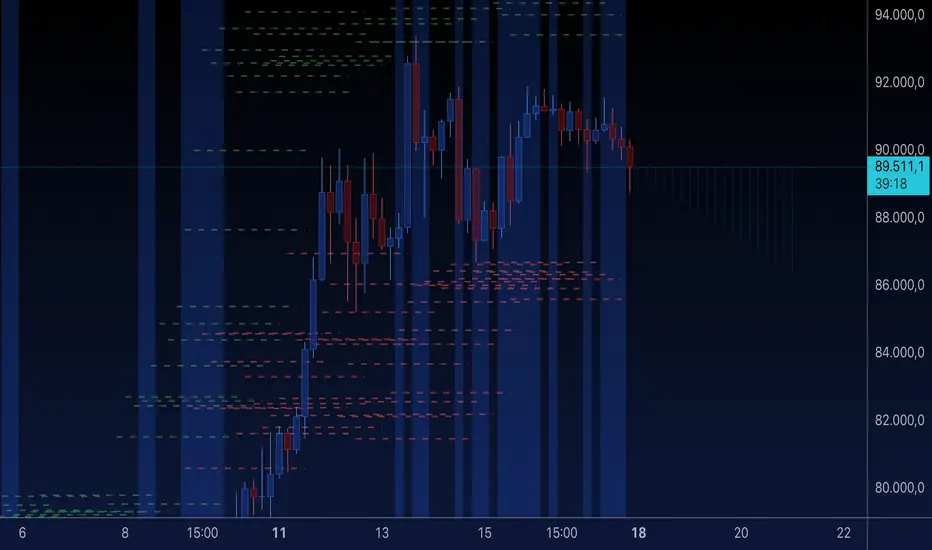
Liquidity Location Detector [BigBeluga]
This indicator helps traders identify potential liquidity zones by detecting significant volume levels at key highs and lows. By using color intensity and scoring numbers, it visually highlights areas where liquidity concentration may be highest while incorporating trend analysis through EMAs.
🔵Key Features:
Liquidity Zone Detection: Automatically detects and marks areas where significant volume has accumulated at swing highs and lows.
Dynamic Box Plotting: Draws liquidity boxes at key highs and lows, updating based on market conditions.
Volume Strength Scaling: Uses a scoring system to rank liquidity zones, helping traders identify the strongest areas.
Color Intensity for Volume Strength: More transperent color indicate less liquidity, while less transperent represent stronger volume concentrations.
Customizable Display: Users can adjust the number of displayed liquidity zones and modify colors to suit their trading style.
Real-Time Liquidity Adaptation: As price interacts with liquidity zones, the indicator updates dynamically to reflect changing market conditions.
Auto-Stopping Liquidity Zones: Liquidity boxes automatically stop extending to the right once price crosses them, preventing outdated zones from interfering with live market action.
Trend Analysis with EMAs: Includes two optional EMAs (fast and slow) to help traders analyze market trends. Users can enable or disable these EMAs in the settings and use crossover signals for trend confirmation.
🔵Usage:
Identify Key Liquidity Areas: Use color intensity and transparency levels to determine high-impact liquidity zones.
Support & Resistance Confirmation: Liquidity zones can act as potential support and resistance levels, enhancing trade decision-making.
Market Structure Analysis: Observe how price interacts with liquidity to anticipate breakout or reversal points.
Scalping & Swing Trading: Works for both short-term and long-term traders looking for liquidity-based trade setups.
Liquidation Map Insight: A liquidity map highlights areas where large amounts of leveraged positions (both long and short) are likely to get liquidated. Since many traders use leverage, sharp price movements can trigger a cascade of liquidations, leading to rapid price surges or drops. Monitoring these liquidity zones and trends helps traders anticipate where price might react strongly.
Liquidity Location Detector is an essential tool for traders seeking to map out potential liquidity zones, providing deeper insights into market structure and trading volume dynamics.

TradFi Fundamentals: Enhanced Macroeconomic Momentum Trading Introduction
The "Enhanced Momentum with Advanced Normalization and Smoothing" indicator is a tool that combines traditional price momentum with a broad range of macroeconomic factors. I introduced the basic version from a research paper in my last script. This one leverages not only the price action of a security but also incorporates key economic data—such as GDP, inflation, unemployment, interest rates, consumer confidence, industrial production, and market volatility (VIX)—to create a comprehensive, normalized momentum score.
Previous indicator
Explanation
In plain terms, the indicator calculates a raw momentum value based on the change in price over a defined lookback period. It then normalizes this momentum, along with several economic indicators, using a method chosen by the user (options include simple, exponential, or weighted moving averages, as well as a median absolute deviation (MAD) approach). Each normalized component is assigned a weight reflecting its relative importance, and these weighted values are summed to produce an overall momentum score.
To reduce noise, the combined momentum score can be further smoothed using a user-selected method.
Signals
For generating trade signals, the indicator offers two modes:
Zero Cross Mode: Signals occur when the smoothed momentum line crosses the zero threshold.
Zone Mode: Overbought and oversold boundaries (which are user defined) provide signals when the momentum line crosses these preset limits.
Definition of the Settings
Price Momentum Settings:
Price Momentum Lookback: The number of days used to compute the percentage change in price (default 50 days).
Normalization Period (Price Momentum): The period over which the price momentum is normalized (default 200 days).
Economic Data Settings:
Normalization Period (Economic Data): The period used to normalize all economic indicators (default 200 days).
Normalization Method: Choose among SMA, EMA, WMA, or MAD to standardize both price and economic data. If MAD is chosen, a multiplier factor is applied (default is 1.4826).
Smoothing Options:
Apply Smoothing: A toggle to enable further smoothing of the combined momentum score.
Smoothing Period & Method: Define the period and type (SMA, EMA, or WMA) used to smooth the final momentum score.
Signal Generation Settings:
Signal Mode: Select whether signals are based on a zero-line crossover or by crossing user-defined overbought/oversold (OB/OS) zones.
OB/OS Zones: Define the upper and lower boundaries (default upper zones at 1.0 and 2.0, lower zones at -1.0 and -2.0) for zone-based signals.
Weights:
Each component (price momentum, GDP, inflation, unemployment, interest rates, consumer confidence, industrial production, and VIX) has an associated weight that determines its contribution to the overall score. These can be adjusted to reflect different market views or risk preferences.
Visual Aspects
The indicator plots the smoothed combined momentum score as a continuous blue line against a dotted zero-line reference. If the Zone signal mode is selected, the indicator also displays the upper and lower OB/OS boundaries as horizontal lines (red for overbought and green for oversold). Buy and sell signals are marked by small labels ("B" for buy and "S" for sell) that appear at the bottom or top of the chart when the score crosses the defined thresholds, allowing traders to quickly identify potential entry or exit points.
Conclusion
This enhanced indicator provides traders with a robust approach to momentum trading by integrating traditional price-based signals with a suite of macroeconomic indicators. Its normalization and smoothing techniques help reduce noise and mitigate the effects of outliers, while the flexible signal generation modes offer multiple ways to interpret market conditions. Overall, this tool is designed to deliver a more nuanced perspective on market momentum.

MMXM ICT [TradingFinder] Market Maker Model PO3 CHoCH/CSID + FVG🔵 Introduction
The MMXM Smart Money Reversal leverages key metrics such as SMT Divergence, Liquidity Sweep, HTF PD Array, Market Structure Shift (MSS) or (ChoCh), CISD, and Fair Value Gap (FVG) to identify critical turning points in the market. Designed for traders aiming to analyze the behavior of major market participants, this setup pinpoints strategic areas for making informed trading decisions.
The document introduces the MMXM model, a trading strategy that identifies market maker activity to predict price movements. The model operates across five distinct stages: original consolidation, price run, smart money reversal, accumulation/distribution, and completion. This systematic approach allows traders to differentiate between buyside and sellside curves, offering a structured framework for interpreting price action.
Market makers play a pivotal role in facilitating these movements by bridging liquidity gaps. They continuously quote bid (buy) and ask (sell) prices for assets, ensuring smooth trading conditions.
By maintaining liquidity, market makers prevent scenarios where buyers are left without sellers and vice versa, making their activity a cornerstone of the MMXM strategy.
SMT Divergence serves as the first signal of a potential trend reversal, arising from discrepancies between the movements of related assets or indices. This divergence is detected when two or more highly correlated assets or indices move in opposite directions, signaling a likely shift in market trends.
Liquidity Sweep occurs when the market targets liquidity in specific zones through false price movements. This process allows major market participants to execute their orders efficiently by collecting the necessary liquidity to enter or exit positions.
The HTF PD Array refers to premium and discount zones on higher timeframes. These zones highlight price levels where the market is in a premium (ideal for selling) or discount (ideal for buying). These areas are identified based on higher timeframe market behavior and guide traders toward lucrative opportunities.
Market Structure Shift (MSS), also referred to as ChoCh, indicates a change in market structure, often marked by breaking key support or resistance levels. This shift confirms the directional movement of the market, signaling the start of a new trend.
CISD (Change in State of Delivery) reflects a transition in price delivery mechanisms. Typically occurring after MSS, CISD confirms the continuation of price movement in the new direction.
Fair Value Gap (FVG) represents zones where price imbalance exists between buyers and sellers. These gaps often act as price targets for filling, offering traders opportunities for entry or exit.
By combining all these metrics, the Smart Money Reversal provides a comprehensive tool for analyzing market behavior and identifying key trading opportunities. It enables traders to anticipate the actions of major players and align their strategies accordingly.
MMBM :
MMSM :
🔵 How to Use
The Smart Money Reversal operates in two primary states: MMBM (Market Maker Buy Model) and MMSM (Market Maker Sell Model). Each state highlights critical structural changes in market trends, focusing on liquidity behavior and price reactions at key levels to offer precise and effective trading opportunities.
The MMXM model expands on this by identifying five distinct stages of market behavior: original consolidation, price run, smart money reversal, accumulation/distribution, and completion. These stages provide traders with a detailed roadmap for interpreting price action and anticipating market maker activity.
🟣 Market Maker Buy Model
In the MMBM state, the market transitions from a bearish trend to a bullish trend. Initially, SMT Divergence between related assets or indices reveals weaknesses in the bearish trend. Subsequently, a Liquidity Sweep collects liquidity from lower levels through false breakouts.
After this, the price reacts to discount zones identified in the HTF PD Array, where major market participants often execute buy orders. The market confirms the bullish trend with a Market Structure Shift (MSS) and a change in price delivery state (CISD). During this phase, an FVG emerges as a key trading opportunity. Traders can open long positions upon a pullback to this FVG zone, capitalizing on the bullish continuation.
🟣 Market Maker Sell Model
In the MMSM state, the market shifts from a bullish trend to a bearish trend. Here, SMT Divergence highlights weaknesses in the bullish trend. A Liquidity Sweep then gathers liquidity from higher levels.
The price reacts to premium zones identified in the HTF PD Array, where major sellers enter the market and reverse the price direction. A Market Structure Shift (MSS) and a change in delivery state (CISD) confirm the bearish trend. The FVG then acts as a target for the price. Traders can initiate short positions upon a pullback to this FVG zone, profiting from the bearish continuation.
Market makers actively bridge liquidity gaps throughout these stages, quoting continuous bid and ask prices for assets. This ensures that trades are executed seamlessly, even during periods of low market participation, and supports the structured progression of the MMXM model.
The price’s reaction to FVG zones in both states provides traders with opportunities to reduce risk and enhance precision. These pullbacks to FVG zones not only represent optimal entry points but also create avenues for maximizing returns with minimal risk.
🔵 Settings
Higher TimeFrame PD Array : Selects the timeframe for identifying premium/discount arrays on higher timeframes.
PD Array Period : Specifies the number of candles for identifying key swing points.
ATR Coefficient Threshold : Defines the threshold for acceptable volatility based on ATR.
Max Swing Back Method : Choose between analyzing all swings ("All") or a fixed number ("Custom").
Max Swing Back : Sets the maximum number of candles to consider for swing analysis (if "Custom" is selected).
Second Symbol for SMT : Specifies the second asset or index for detecting SMT divergence.
SMT Fractal Periods : Sets the number of candles required to identify SMT fractals.
FVG Validity Period : Defines the validity duration for FVG zones.
MSS Validity Period : Sets the validity duration for MSS zones.
FVG Filter : Activates filtering for FVG zones based on width.
FVG Filter Type : Selects the filtering level from "Very Aggressive" to "Very Defensive."
Mitigation Level FVG : Determines the level within the FVG zone (proximal, 50%, or distal) that price reacts to.
Demand FVG : Enables the display of demand FVG zones.
Supply FVG : Enables the display of supply FVG zones.
Zone Colors : Allows customization of colors for demand and supply FVG zones.
Bottom Line & Label : Enables or disables the SMT divergence line and label from the bottom.
Top Line & Label : Enables or disables the SMT divergence line and label from the top.
Show All HTF Levels : Displays all premium/discount levels on higher timeframes.
High/Low Levels : Activates the display of high/low levels.
Color Options : Customizes the colors for high/low lines and labels.
Show All MSS Levels : Enables display of all MSS zones.
High/Low MSS Levels : Activates the display of high/low MSS levels.
Color Options : Customizes the colors for MSS lines and labels.
🔵 Conclusion
The Smart Money Reversal model represents one of the most advanced tools for technical analysis, enabling traders to identify critical market turning points. By leveraging metrics such as SMT Divergence, Liquidity Sweep, HTF PD Array, MSS, CISD, and FVG, traders can predict future price movements with precision.
The price’s interaction with key zones such as PD Array and FVG, combined with pullbacks to imbalance areas, offers exceptional opportunities with favorable risk-to-reward ratios. This approach empowers traders to analyze the behavior of major market participants and adopt professional strategies for entry and exit.
By employing this analytical framework, traders can reduce errors, make more informed decisions, and capitalize on profitable opportunities. The Smart Money Reversal focuses on liquidity behavior and structural changes, making it an indispensable tool for financial market success.

BRT Cluster VolumeTitle and Purpose
BRT Cluster Volume is a powerful market analysis tool designed to identify key support and resistance levels, cluster volumes, and breakout signals. This script is highly beneficial for traders who aim to gain deeper insights into market trends and pinpoint zones of interest for buyers and sellers.
Key Features
1. Support and Resistance Levels:
- The script automatically detects chart extremums by analyzing a specified number of bars on the left and right to form levels. This approach effectively identifies local highs and lows.
- The uniqueness of this implementation lies in its dynamic data processing. For each extremum, the "channel width" is calculated, allowing insignificant levels to be filtered out based on a user-defined minimum width. This method eliminates noise and ensures focus on critical levels.
- Extremum lines can be extended to the right (when enabled), allowing traders to track current price movements relative to historical levels.
2. Cluster Volume:
- The cluster analysis is based on lower timeframe data, providing precise identification of key zones of market participant activity. The script dynamically requests close prices and volumes from lower timeframes, calculates the average volume, and identifies levels where volumes exceed a defined threshold.
- The visualization of cluster volumes is unique: volumes exceeding the threshold are displayed as candles with customizable colors and markers. These indicators help traders identify zones of significant interest.
- Cluster volume is only displayed when it interacts with support or resistance levels, ensuring that the visualization remains precise and relevant for market analysis.
3. Breakout Signals:
- The script evaluates "breakout strength" for each breakout of support or resistance levels by comparing the current price with the level. This helps filter false breakouts and focus on significant price movements.
- Traders can select the source for breakout signals (close price or high/low), offering flexibility for various trading styles and strategies.
- By incorporating the concept of "maximum breakout strength," the script highlights only meaningful breakouts, ignoring minor fluctuations.
4. Integration of Trading Sessions:
- Extremum levels for major trading sessions (Asia, Europe, USA) are identified and labeled on the chart. This allows traders to see when significant price levels were formed during the day.
- The script uses timestamps to automatically detect session times, ensuring accuracy and minimizing manual adjustments.
5. Dynamic Data Updates:
- The script dynamically updates support and resistance levels in real time as new data becomes available. This feature is crucial for traders working in fast-moving markets.
- Outdated information (such as obsolete levels) is automatically removed to keep the chart clean and focused on relevant data.
6. Visualization of Activity Zones:
- Trend direction is visualized using color-coded candles based on cluster volumes. For instance, candles with volumes exceeding the average are highlighted with specific colors, helping traders quickly identify areas of heightened activity.
- The unique aspect of this visualization is that cluster volumes appear only in zones where they interact with breakout levels, providing an intuitive and streamlined presentation of critical data.
Usage
- Support and Resistance: Adjust the "Left Bars" and "Right Bars" settings to determine extremums. Use the "Channel Min Width" setting to filter out insignificant levels.
- Cluster Volume: Customize the analysis period and volume threshold to identify high-activity zones. Enable breakout clusters to see how volumes interact with breakouts.
- Session Extremums: Highlight significant levels for Asia, Europe, and US trading sessions to gain insights into market dynamics across different time zones.
- Breakout Signals: Configure the breakout strength and source (close or high/low) for precise signal detection.
Parameter Details
1. Support & Resistance:
- `Left Bars` / `Right Bars`: Number of bars to consider for determining extremums.
- `# of Lines`: Maximum number of support/resistance lines to display.
- `Channel Min Width`: Minimum channel width to filter insignificant levels.
2. Breakout:
- `Show Breakouts`: Toggle breakout signal display.
- `Max breakout strength`: Maximum strength for valid breakouts.
- `Breakout source`: Data source for breakouts (close or high/low).
3. Cluster Volume:
- `Lookback`: Number of bars to analyze for cluster volumes.
- `Threshold`: Volume threshold (percentage above the average).
- `Cluster Volume Timeframe`: Timeframe for cluster volume analysis.
- `Breakout Cluster`: Display cluster volumes only for breakout-related zones.
4. Visual Settings:
- `Extend extremum lines to the right`: Extend support/resistance lines to the right.
- `Show ASIA/EU/US Session Extremums`: Display extremums for trading sessions.
Features and Benefits
- The script provides flexible parameter customization, allowing it to adapt to different trading styles and timeframes.
- The visualization is designed to be clean and intuitive, ensuring users can easily interpret the data.
- Suitable for all timeframes, making it ideal for both intraday and long-term market analysis.
Limitations
- The script is not suitable for analysis on non-standard chart types (e.g., Heikin Ashi, Renko, Kagi).
- To ensure accurate performance, realistic data for commission and slippage should be used.
Warnings
- The script relies on historical data for calculations, which may cause discrepancies in real-time conditions.
- Users should fully understand the functionality of cluster analysis and breakout signals before using the script in live trading.
This script combines advanced data processing logic, dynamic level adjustments, and unique visualization approaches, making it an indispensable tool for market analysis and trading decision-making.

Infinity Market Grid -AynetConcept
Imagine viewing the market as a dynamic grid where price, time, and momentum intersect to reveal infinite possibilities. This indicator leverages:
Grid-Based Market Flow: Visualizes price action as a grid with zones for:
Accumulation
Distribution
Breakout Expansion
Volatility Compression
Predictive Dynamic Layers:
Forecasts future price zones using historical volatility and momentum.
Tracks event probabilities like breakout, fakeout, and trend reversals.
Data Science Visuals:
Uses heatmap-style layers, moving waveforms, and price trajectory paths.
Interactive Alerts:
Real-time alerts for high-probability market events.
Marks critical zones for "buy," "sell," or "wait."
Key Features
Market Layers Grid:
Creates dynamic "boxes" around price using fractals and ATR-based volatility.
These boxes show potential future price zones and probabilities.
Volatility and Momentum Waves:
Overlay volatility oscillators and momentum bands for directional context.
Dynamic Heatmap Zones:
Colors the chart dynamically based on breakout probabilities and risk.
Price Path Prediction:
Tracks price trajectory as a moving "wave" across the grid.
How It Works
Grid Box Structure:
Upper and lower price levels are based on ATR (volatility) and plotted dynamically.
Dashed green/red lines show the grid for potential price expansion zones.
Heatmap Zones:
Colors the background based on probabilities:
Green: High breakout probability.
Blue: High consolidation probability.
Price Path Prediction:
Forecasts future price movements using momentum.
Plots these as a dynamic "wave" on the chart.
Momentum and Volatility Waves:
Shows the relationship between momentum and volatility as oscillating waves.
Helps identify when momentum exceeds volatility (potential breakouts).
Buy/Sell Signals:
Triggers when price approaches grid edges with strong momentum.
Provides alerts and visual markers.
Why Is It Revolutionary?
Grid and Wave Synergy:
Combines structural price zones (grid boxes) with real-time momentum and volatility waves.
Predictive Analytics:
Uses momentum-based forecasting to visualize what’s next, not just what’s happening.
Dynamic Heatmap:
Creates a living map of breakout/consolidation zones in real-time.
Scalable for Any Market:
Works seamlessly with forex, crypto, and stocks by adjusting the ATR multiplier and box length.
This indicator is not just a tool but a framework for understanding market dynamics at a deeper level. Let me know if you'd like to take it even further — for example, adding machine learning-inspired probability models or multi-timeframe analysis! 🚀
Fractal Trend Detector [Skyrexio]Introduction
Fractal Trend Detector leverages the combination of Williams fractals and Alligator Indicator to help traders to understand with the high probability what is the current trend: bullish or bearish. It visualizes the potential uptrend with the coloring bars in green, downtrend - in red color. Indicator also contains two additional visualizations, the strong uptrend and downtrend as the green and red zones and the white line - trend invalidation level (more information in "Methodology and it's justification" paragraph)
Features
Optional strong up and downtrends visualization: with the specified parameter in settings user can add/hide the green and red zones of the strong up and downtrends.
Optional trend invalidation level visualization: with the specified parameter in settings user can add/hide the white line which shows the current trend invalidation price.
Alerts: user can set up the alert and have notifications when uptrend/downtrend has been started, strong uptrend/downtrend started.
Methodology and it's justification
In this script we apply the concept of trend given by Bill Williams in his book "Trading Chaos". This approach leverages the Alligator and Fractals in conjunction. Let's briefly explain these two components.
The Williams Alligator, created by Bill Williams, is a technical analysis tool used to identify trends and potential market reversals. It consists of three moving averages, called the jaw, teeth, and lips, which represent different time periods:
Jaw (Blue Line): The slowest line, showing a 13-period smoothed moving average shifted 8 bars forward.
Teeth (Red Line): The medium-speed line, an 8-period smoothed moving average shifted 5 bars forward.
Lips (Green Line): The fastest line, a 5-period smoothed moving average shifted 3 bars forward.
When the lines are spread apart and aligned, the "alligator" is "awake," indicating a strong trend. When the lines intertwine, the "alligator" is "sleeping," signaling a non-trending or range-bound market. This indicator helps traders identify when to enter or avoid trades.
Williams Fractals, introduced by Bill Williams, are a technical analysis tool used to identify potential reversal points on a price chart. A fractal is a series of at least five consecutive bars where the middle bar has the highest high (for a up fractal) or the lowest low (for a down fractal), compared to the two bars on either side.
Key Points:
Up fractal: Formed when the middle bar shows a higher high than the two preceding and two following bars, signaling a potential turning point downward.
Down fractal: Formed when the middle bar has a lower low than the two surrounding bars, indicating a potential upward reversal.
Fractals are often used with other indicators to confirm trend direction or reversal, helping traders make more informed trading decisions.
How we can use its combination? Let's explain the uptrend example. The up fractal breakout to the upside can be interpret as bullish sign, there is a high probability that uptrend has just been started. It can be explained as following: the up fractal created is the potential change in market's behavior. A lot of traders made a decision to sell and it created the pullback with the fractal at the top. But if price is able to reach the fractal's top and break it, this is a high probability sign that market "changed his opinion" and bullish trend has been started. The moment of breaking is the potential changing to the uptrend. Here is another one important point, this breakout shall happen above the Alligator's teeth line. If not, this crossover doesn't count and the downtrend potentially remaining. The inverted logic is true for the down fractals and downtrend.
According to this methodology we received the high probability up and downtrend changes, but we can even add it. If current trend established by the indicator as the uptrend and alligator's lines have the following order: lips is higher than teeth, teeth is higher than jaw, script count it as a strong uptrend and start print the green zone - zone between lips and jaw. It can be used as a high probability support of the current bull market. The inverted logic can be used for bearish trend and red zones: if lips is lower than teeth and teeth is lower than jaw it's interpreted by the indicator as a strong down trend.
Indicator also has the trend invalidation line (white line). If current bar is green and market condition is interpreted by the script as an uptrend you will see the invalidation line below current price. This is the price level which shall be crossed by the price to change up trend to down trend according to algorithm. This level is recalculated on every candle. The inverted logic is valid for downtrend.
How to use indicator
Apply it to desired chart and time frame. It works on every time frame.
Setup the settings with enabling/disabling visualization of strong up/downtrend zones and trend invalidation line. "Show Strong Bullish/Bearish Trends" and "Show Trend Invalidation Price" checkboxes in the settings. By default they are turned on.
Analyze the price action. Indicator colored candle in green if it's more likely that current state is uptrend, in red if downtrend has the high probability to be now. Green zones between two lines showing if current uptrend is likely to be strong. This zone can be used as a high probability support on the uptrend. The red zone show high probability of strong downtrend and can be used as a resistance. White line is showing the level where uptrend or downtrend is going be invalidated according to indicator's algorithm. If current bar is green invalidation line will be below the current price, if red - above the current price.
Set up the alerts if it's needed. Indicator has four custom alerts called "Uptrend has been started" when current bar closed as green and the previous was not green, "Downtrend has been started" when current bar closed red and the previous was not red, "Uptrend became strong" if script started printing the green zone "Downtrend became strong" if script started printing the red zone.
Disclaimer:
Educational and informational tool reflecting Skyrex commitment to informed trading. Past performance does not guarantee future results. Test indicators before live implementation.

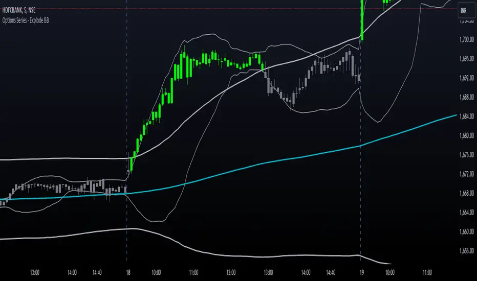
Options Series - Explode BB⭐ Bullish Zone:
⭐ Bearish Zone:
⭐ Neutral Zone:
The provided script integrates Bollinger Bands with different lengths (20 and 200 periods) and applies customized candle coloring based on certain conditions. Here's a breakdown of its importance and insights:
⭐ 1. Dual Bollinger Bands (BBs):
Bollinger Bands (BB) with 20-period length:
This is the standard setting for Bollinger Bands, with a 20-period simple moving average (SMA) as the central line and upper/lower bands derived from the standard deviation.
These bands are used to identify volatility. Wider bands indicate higher volatility, while narrower bands indicate low volatility.
200-period BB:
This is a longer-term indicator providing insight into the overall trend and long-term volatility.
The 200-period bands filter out noise and offer a "macro" view of price movements compared to the 20-period bands, which focus on short-term price actions.
⭐ 2. Overlay of Bollinger Bands and SMA:
The script plots the Bollinger Bands along with the SMA (Simple Moving Average) of the 200-period BB. This gives traders both a short-term (20-period) and long-term (200-period) perspective, which is valuable for detecting major trend shifts or key support and resistance zones.
Using multiple time frames (20-period for short-term and 200-period for long-term) can help traders spot both immediate opportunities and overarching trends.
⭐ 3. Candle Coloring Based on Key Conditions:
Bullish Signal (GreenFluroscent): When the price closes above the upper 200-period Bollinger Band, the candle turns green, indicating a potential bullish breakout.
Bearish Signal (RedFluroscent): If the price closes below the lower 200-period Bollinger Band, the candle turns red, suggesting a bearish breakout.
Neutral or Uncertain Market: Candles are gray when the price remains between the upper and lower bands, indicating a lack of a strong directional bias.
This color-coded visualization allows traders to quickly assess market sentiment based on the Bollinger Bands' extremes.
⭐ 4. Strategic Importance of the Setup:
Multi-timeframe Analysis: Combining short-term (20-period) and long-term (200-period) Bollinger Bands enables traders to assess the market's overall volatility and trend strength. The longer-term bands act as a reference for broader trend direction, while the shorter-term bands can signal shorter-term pullbacks or entry/exit points.
Breakout Identification: By color-coding the candles when prices cross either the upper or lower 200-period bands, the script makes it easier to spot potential breakouts. This can be particularly helpful in trading strategies that rely on volatility expansions or trend-following tactics.
⭐ 5. Customization and Flexibility:
Custom Colors: The script uses distinct fluorescent green and red colors to highlight key bullish and bearish conditions, providing clear visual cues.
Simplicity with Flexibility: Despite its simplicity, the script leaves room for customization, allowing traders to adjust the Bollinger Band multipliers or apply different conditions to candle coloring for more nuanced setups.
This script enhances standard Bollinger Band usage by introducing multi-timeframe analysis, breakout signals, and visual cues for trend strength, making it a powerful tool for both trend-following and mean-reversion strategies.
🚀 Conclusion:
This script effectively simplifies volatility analysis by visually marking bullish, bearish, and neutral zones, making it a robust tool for identifying trade opportunities across multiple timeframes. Its dual-band approach ensures both trend-following and mean-reversion strategies are supported.
Fractal Levels [BigBeluga]The Fractal Levels - BigBeluga indicator is a specialized tool that detects significant market highs and lows, ranking them by their normalized volume. This indicator is designed to help traders identify crucial price levels that are likely to influence market behavior, enabling better decision-making in trading. By gathering normalized volume around each fractal point, it creates a comprehensive view of the strength and relevance of price reversal points, which can be visualized as numbers or zones on the chart.
🔵KEY FEATURES & USAGE
● High and Low Detection with Volume Ranking:
The indicator detects market highs and lows using a user-defined length setting. For each detected fractal point (high or low), it collects normalized volume from a set number of bars before and after the fractal point (the number is based on the length input). This collection allows the indicator to produce an average of the normalized volume, which is then displayed as a number above or below the corresponding fractal arrows, visually indicating the importance of the high or low.
● Plotting Levels from Fractals:
From these high and low points, the indicator plots key levels. In settings, traders can choose between a wide or tight zone type.
If a price level coincides with multiple pivot points, the indicator highlights this as a significant zone. These zones represent areas where price tends to react, making them critical for identifying potential support and resistance levels.
● Fractal Boxes with Delta Volume Data:
Fractal boxes are shown as gray boxes, representing areas where price pivots occurred, and they also contain delta volume information. Delta volume is calculated by summing the positive and negative volumes within the length range, producing the total delta inside each fractal box. This is particularly useful for analyzing volume shifts around key levels.
● Broken Levels Highlighting:
When a plotted level is broken (price closes above or below it), the level can be removed from the chart automatically. However, in the settings, you can enable a feature to highlight broken levels as gray areas, providing insight into past price behavior. This is helpful for tracking historical support and resistance zones.
> Important note: If no volume data provided indicator wont work
🔵 CUSTOMIZATION
Fractal Length and Filter Settings:
Adjust the Length parameter to control the number of bars used to detect pivot highs and lows. A longer length will result in fewer fractals being identified, focusing on more significant price moves. The Filter option allows you to set a volume threshold, filtering out minor fractals that do not meet the minimum volume requirements.
Levels Detection (Wide or Tight):
Choose between Wide and Tight zones for fractal levels detection. A tight zone focuses on smaller price areas around pivot points, while a wide zone expands the detection range, highlighting larger zones of influence around fractals.
Delta Volume Display for Fractals:
Toggle Delta Volume Fractals to show or hide the delta volume information inside fractal boxes. When enabled, the indicator calculates and displays the total delta volume within the range of bars surrounding each fractal point.
Broken Levels Visibility:
Enable Broken Levels to highlight levels that have been crossed by price. When disabled, broken fractal levels will be removed from the chart after price crosses them.
🔵CONCLUSION
The Fractal Levels indicator provides traders with an advanced way to analyze price highs and lows by combining fractal detection with volume dynamics. By identifying key market levels through normalized volume ranking, delta volume analysis, and level plotting, this tool is invaluable for spotting potential support and resistance zones. Whether you're focusing on short-term trading or longer-term price movements, Fractal Levels offers the precision and flexibility needed to optimize your strategy.

LRS-Strategy: 200-EMA Buffer & Long/Short Signals LRS-Strategy: 200-EMA Buffer & Long/Short Signals
This indicator is designed to help traders implement the Leveraged Return Strategy (LRS) using the 200-day Exponential Moving Average (EMA) as a key trend-following signal. The indicator offers clear long and short signals by analyzing the price movements relative to the 200-day EMA, enhanced by customizable buffer zones for increased precision.
Key Features:
200-Day EMA: The main trend indicator. When the price is above the 200-day EMA, the market is considered in an uptrend, and when it is below, it indicates a downtrend.
Customizable Buffer Zones: Users can define a percentage buffer around the 200-day EMA (default is 3%). The upper and lower buffer zones help filter out noise and prevent premature signals.
Precise Long/Short Signals:
Long Signal: Triggered when the price moves from below the lower buffer zone, crosses the 200-day EMA, and then breaks above the upper buffer zone.
Short Signal: Triggered when the price moves from above the upper buffer zone, crosses the 200-day EMA, and then breaks below the lower buffer zone.
Alternating Signals: Ensures that a new signal (long or short) is only generated after the opposite signal has been triggered, preventing multiple signals of the same type without a reversal.
Clear Visual Aids: The indicator displays the 200-day EMA and buffer zones on the chart, along with buy (long) and sell (short) signals. This makes it easy to track trends and time entries/exits.
How to Use:
Long Entry: Look for the price to move below the lower buffer, cross the 200-day EMA from below, and then break out of the upper buffer to confirm a long signal.
Short Entry: Look for the price to move above the upper buffer, cross below the 200-day EMA, and then break below the lower buffer to confirm a short signal.
This indicator is perfect for traders who prefer a structured, trend-following approach, using clear rules to minimize noise and identify meaningful long or short opportunities.

Ultra SessionsThe "Ultra Sessions" indicator is designed to enhance your trading strategy by clearly marking key market sessions and their associated "kill zones" directly on your chart. This powerful tool supports multiple time zones and provides customizable alerts for session opens, closes, and critical kill zones, ensuring you never miss important market movements.
Customizable Time Zones: Align the indicator with your local time by selecting from a wide range of global time zones.
Market Session Tracking: Visually track the New York, London, and Tokyo trading sessions with distinct color-coded markers.
Kill Zones: Highlight the high-volatility periods within each session to focus on key trading opportunities.
Alert System: Receive real-time alerts for session openings, closings, and kill zones, so you stay informed without constantly monitoring the chart.
Flexible Positioning: Choose the positioning of session markers to fit your chart layout, whether at the top or bottom.
Ideal for traders who want to optimize their entry and exit points by focusing on the most active and volatile times in the market, the indicator is a must-have for any serious trading setup.

Indecisive and Explosive CandlesThe Explosive & Base Candle with Gaps Identifier is an indicator designed to enhance your market analysis by identifying critical candle types and gaps in price action. This tool aids traders in pinpointing zones of significant buyer-seller interaction and potential institutional activity, providing valuable insights for strategic trading decisions.
Main Features:
Base Candle Identification: This feature detects Base candles, also known as indecisive candles, within the price action. A Base candle is characterized by a body (the difference between the close and open prices) that is less than or equal to 50% of its total range (the difference between the high and low prices). These candles mark zones where buyers and sellers are evenly matched, highlighting areas of potential support and resistance.
Explosive Candle Identification: The indicator identifies Explosive candles, which are indicative of strong market moves often driven by institutional activity. An Explosive candle is defined by a body that is greater than 70% of its total range. Recognizing these candles helps traders spot significant momentum and potential breakout points.
Supply and Demand Zone Identification: Both Base and Explosive candles are essential for identifying supply and demand zones within the price action. These zones are crucial for traders to place their trades based on the likelihood of price reversals or continuations.
Gap Detection: The indicator also detects gaps, defined as the difference between the close price of one candle and the open price of the next. Gaps are significant because prices often return to these levels to "fill the gap," providing opportunities for traders to predict price movements and place strategic trades.
Visual Markings and Alerts: The indicator visually marks Base and Explosive candles as well as gaps directly on the chart, making them easily identifiable at a glance. Traders can also set customizable alerts to notify them when these key candle types and gaps appear, ensuring they never miss an important trading opportunity.
Customizable Settings: Tailor the indicator’s settings to match your trading style and preferences. Adjust the criteria for Base and Explosive candles, as well as how gaps are detected and displayed, to suit your specific analysis needs.
How to Use:
Add the Indicator: Apply the Explosive & Base Candle with Gaps Identifier to your TradingView chart.
Analyze Identified Zones: Observe the marked Base and Explosive candles and gaps to identify key areas of support, resistance, and potential price reversals or continuations.
Set Alerts: Customize and set alerts for the detection of Base candles, Explosive candles, and gaps to stay informed of critical market movements in real-time.
Integrate with Your Strategy: Use the insights provided by the indicator to enhance your existing trading strategy, improving your entry and exit points based on the identified supply and demand zones.
The Explosive & Base Candle with Gaps Identifier is an invaluable tool for traders aiming to refine their market analysis and make more informed trading decisions. By identifying critical areas of price action, this indicator supports traders in navigating the complexities of the financial markets with greater precision and confidence.
Inversion Fair Value Gap Consumption | Flux Charts💎 GENERAL OVERVIEW
Introducing our new Inversion Fair Value Gap Consumption (IFVG) indicator! Inversion Fair Value Gaps occur when a Fair Value Gap becomes invalidated. They reverse the role of the original Fair Value Gap, making a bullish zone bearish and vice versa. IFVGs get "consumed" when market orders fill the gap occurred. With this indicator, you can now see the percentage of the IFVG's consumed part. For more information about the process, read the "HOW DOES IT WORK" section of the description.
Features of the new Consumption IFVG Indicator :
Render Bullish / Bearish IFVG Zones
See The Consumed Part Of The IFVG Zones
Combination Of Overlapping FVG Zones
Variety Of Zone Detection / Sensitivity / Filtering / Invalidation Settings
High Customizability
🚩UNIQUENESS
This indicator stands out with its ability to render the consumed part of IFVGs. You can see how much of the IFVG's gap is filled, with it's percentage. Also the ability to combine overlapping FVG zones will result in cleaner charts for traders. You can customize the FVG Filtering method, FVG & IFVG Zone Invalidation, Detection Sensitivity etc. according to your needs to get the best performance from the indicator.
📌 HOW DOES IT WORK ?
A Fair Value Gap generally occur when there is an imbalance in the market. They can be detected by specific formations within the chart. An Inversion Fair Value Gap is when a FVG becomes invalidated, thus reversing the direction of the FVG.
IFVGs get consumed when a Close / Wick enters the IFVG zone. Check this example:
⚙️SETTINGS
1. General Configuration
FVG Zone Invalidation -> Select between Wick & Close price for FVG Zone Invalidation.
IFVG Zone Invalidation -> Select between Wick & Close price for IFVG Zone Invalidation. This setting also switches the type for IFVG consumption.
Zone Filtering -> With "Average Range" selected, algorithm will find FVG zones in comparison with average range of last bars in the chart. With the "Volume Threshold" option, you may select a Volume Threshold % to spot FVGs with a larger total volume than average.
FVG Detection -> With the "Same Type" option, all 3 bars that formed the FVG should be the same type. (Bullish / Bearish). If the "All" option is selected, bar types may vary between Bullish / Bearish.
Detection Sensitivity -> You may select between Low, Normal or High FVG detection sensitivity. This will essentially determine the size of the spotted FVGs, with lower sensitivies resulting in spotting bigger FVGs, and higher sensitivies resulting in spotting all sizes of FVGs.
Show Historic Zones -> If this option is on, the indicator will render invalidated IFVG zones as well as current IFVG zones. For a cleaner look at current IFVG zones which are not invalidated yet, you can turn this option off.

Session Sweeps [LuxAlgo]The Session Sweeps indicator combines ICT-based features for a complete trading methodology involving market sessions, market structure, and fair value gaps to find optimal entry conditions for trading price action.
Traders frequently tend to place stop/limit orders at the high and low points of major trading sessions such as Asian (Tokyo), European (London), and North American (New York), resulting in the establishment of liquidity pools at those particular levels. The Session Sweeps indicator is crafted to recognize and underscore occurrences of session sweeps or liquidity sweeps during these major trading sessions.
🔶 USAGE
Default settings utilize major forex trading sessions, yet users can select their preferred opening and closing times, rename the sessions, or adjust the colors. It's important to note that the specified times for each session align with the respective local timezones: Asian (Tokyo) UTC+9, European (London) UTC, and North American (New York) UTC-5.
If the price briefly crosses either the highest or lowest point of a market session. These movements, aiming at triggering stop losses, suggest potential shifts in the market direction. Detecting such movements is the fundamental purpose and core functionality of the script.
🔹Market Structure Shifts
A Market Structure Shift refers to a change in market direction, either from an uptrend to a downtrend or vice versa. A part of a common entry model when using session sweeps is waiting for the formation of a CHoCH after a session sweep.
🔹Fair Value Gaps
A Fair Value Gap (FVG) holds particular appeal for price action traders, emerging when there are inefficiencies or imbalances in the market, often a result of uneven buying and selling activity. The underlying concept of FVGs is that the market tends to revisit these inefficiencies before resuming its trajectory in alignment with the initial impulsive move.
After the formation of a CHoCH traders can enter a position when the price enters the area of a Fair Value Gap (FVG).
🔹Setup Examples
This entry setup is commonly used by ICT traders and is shared for informational & educational purposes only.
Long Positions (5-Minute Timeframe):
Wait for the previous session's low to be swept.
Look for a Bullish Choch.
Find a Bullish FVG formed by or before the Choch.
Entry Point: At the FVG.
Take Profit (TP): At the session high or aim for a 1:2 Risk-Reward Ratio.
Stop Loss (SL): At the session low or nearest Swing Low.
Take partial profits at intermediate swings, but don’t shift SL prematurely.
Short Positions (5-Minute Timeframe):
Wait for the previous session's high to be swept.
Look for a Bearish Choch.
Find a FVG formed by or before the Choch.
Entry Point: At the FVG.
Take Profit (TP): At the previous session's low or aim for a 1:2 RR.
Stop Loss (SL): At the session high or nearest Swing High.
Take partial profits at intermediate swings, but don’t shift SL prematurely.
🔶 SETTINGS
🔹Session Sweeps
Buyside Sweep Zones, Color, and Margin: toggles the visibility of bullside sweep zones, customizes the associated color, and sets the margin value defining the range of a bullside sweep zone.
Sellside Sweep Zones, Color, and Margin: toggles the visibility of sell-side sweep zones, customizes the associated color, and sets the margin value defining the range of a sell-side sweep zone.
Sweep Margin Length: specifies the maximum allowed length of a sweep zone invalidation, the length over which the price slightly invalidated the margin range.
Detect Sweeps Once per Session: if enabled will detect only once a sweep zone within a session.
Hide Fake Sweep Zones, and Color: controls the visibility and color of the fake sweep zones.
🔹Sessions
Session (Asia, London, New York AM, and New York PM), Start Time, and End Time: enables or disables the visibility of the named market session range, and customization of the session hours.
Color: color customization option of the named session.
Extend Max/Min: extends the highest and lowest price levels of the named session until the end of the next enabled session. This option is recommended to be enabled when sweep zone detection is activated to observe the relationship between the sweep zone and previous session extreme levels.
Extend Mid: extends the mean price levels of the named session until the end of the next enabled session. The extended line may serve as potential support and resistance levels.
Fill: enables/disables background coloring of the named session.
New York DST | London DST: enabling this option initiates Daylight Saving Time (DST) for New York or London. Note: Daylight Saving Time is not applied to the Asian (Tokyo) session.
Sessions Extreme Lines | Sessions Names: toggles the visibility of the highest and lowest price levels, as well as the names, for all market sessions.
Session Lines Width: sets the width of the lines for all sessions.
Session Fill Transparency: sets the background color transparency of the range for all sessions.
🔹Market Structure Shifts
Market Structure Shifts: toggles the visibility of market structure shifts, also known as change of character (CHoCH).
Detection Length: specifies the detection length.
Market Structure Shifts; Bull & Bear: color customization options.
🔹Fair Value Gaps
Fair Value Gaps: toggles the visibility of the fair value gaps.
Fair Value Gap Width Filter: specifies the filtering multiplier; additional details can be found in the tooltip of the respective input option.
Bullish & Bearish Imbalance: color customization options.
🔹Sessions Tabular View
Sessions Tabular View: toggles the visibility of the tabular view of the sessions, displaying date &time, status, and countdown counter.
Hide if not Forex Market Instrument: checks the market and automatically enables/disables the option based on the market instrument.
Table Text Size & Position: size and placement customization options
🔶 LIMITATIONS
Please be aware that fair value gap filtering cannot be applied to the initial 144 candles (with a fixed-length ATR) as the ATR value necessary for filtering won't be available during this period.
🔶 RELATED SCRIPTS
Buyside-Sellside-Liquidity
Sessions
Liquidity-Voids-FVG
Thank you to our community for the recommendation of this script. To explore additional conceptual scripts and related content, we invite you to visit >>> LuxAlgo-Scripts .

Support Resistance with Touch HighlightDescription:
Support Resistance with Touch Highlight is a powerful technical analysis tool designed to help traders identify key support and resistance levels in the market. Unlike traditional support and resistance indicators, this indicator utilizes a unique approach by considering multiple periods simultaneously, enhancing its accuracy and reliability.
Key Features:
- **Multi-Period Analysis:** The indicator analyzes multiple user-defined periods, allowing for a comprehensive view of support and resistance levels.
- **Average Calculation:** It calculates the average of the highest and lowest prices within the specified periods, providing a balanced representation of support and resistance zones.
- **Dynamic Highlighting:** Bars touching the support or resistance lines are highlighted, aiding traders in spotting potential reversal points.
- **Alert System:** Set custom alerts to be notified when the price touches the support or resistance lines, enabling timely decision-making.
Why It's Superior:
1. **Accuracy Through Multiple Periods:** By considering multiple periods, the indicator provides a more accurate depiction of support and resistance levels, minimizing false signals.
2. **Dynamic Highlighting:** The indicator dynamically highlights relevant bars, making it easy for traders to identify significant price interactions with support and resistance zones.
3. **Customizable Alerts:** Tailor alerts to your trading strategy, ensuring you never miss crucial market movements.
How to Use:
- **Support Zones:** Prices often bounce off the support line. Look for buying opportunities when the price touches or approaches the green support line.
- **Resistance Zones:** Prices tend to reverse near the resistance line. Consider selling or tightening stops when the price touches or nears the red resistance line.
Disclaimer:
Trading involves risk, and past performance is not indicative of future results. Always perform your analysis and consider risk management strategies before making trading decisions.

GDCA ScreenerThis is upgrated system for Screener to DCA from "Grospector DCA V.3".
This has 5 zone Extreme high , high , normal , low , Extreme low. You can dynamic set min - max percent every zone.
Extreme zone is derivative short and long which It change Extreme zone to Normal zone all position will be closed.
Every Zone is splitted 10 channel. and this strategy calculate contribution.
and now can predict price in future.
Price Type: Allows the user to select the price type (open, high, low, close) for calculations.
ALL SET
Length MA for normal zone: The length of the moving average used in the normal zone.
Length for strong zone: The length of the moving average used in the strong zone, which is averaged from the normal zone moving average.
Multiple for Short: The multiplication factor applied to determine the threshold for the short zone.
Multiple for Strong Sell: The multiplication factor applied to determine the threshold for the strong sell zone.
Multiple for Sell Zone: The multiplication factor applied to determine the threshold for the sell zone.
Multiple for Buy Zone: The multiplication factor applied to determine the threshold for the buy zone.
Multiple for Strong Buy: The multiplication factor applied to determine the threshold for the strong buy zone.
Multiple for Long: The multiplication factor applied to determine the threshold for the long zone.
ZONE
Start Short Zone %: The start percentage of the short zone.
End Short Zone %: The end percentage of the short zone.
Start Sell Zone %: The start percentage of the sell zone.
End Sell Zone %: The end percentage of the sell zone.
Start Normal Zone %: The start percentage of the normal zone.
End Normal Zone %: The end percentage of the normal zone.
Start Buy Zone %: The start percentage of the buy zone.
End Buy Zone %: The end percentage of the buy zone.
Start Long Zone %: The start percentage of the long zone.
End Long Zone %: The end percentage of the long zone.
DISPLAY
Show Price: Controls the visibility of the price column in the display table.
Show Mode: Controls the visibility of the mode column in the display table.
Show GDCA: Controls the visibility of the GDCA column in the display table.
Show %: Controls the visibility of the percentage column in the display table.
Show Short: Controls the visibility of the short column in the display table.
Show Strong Sell: Controls the visibility of the strong sell column in the display table.
Show Sell: Controls the visibility of the sell column in the display table.
Show Buy: Controls the visibility of the buy column in the display table.
Show Strong Buy: Controls the visibility of the strong buy column in the display table.
Show Long: Controls the visibility of the long column in the display table.
Show Suggestion Trend: Controls the visibility of the suggestion trend column in the display table.
Show Manual Custom Code: Controls the visibility of the manual custom code column in the display table.
Show Dynamic Trend: Controls the visibility of the dynamic trend column in the display table.
Symbols: Boolean parameters that control the visibility of individual symbols in the display table.
Mode: Integer parameters that determine the mode for each symbol, specifying different settings or trends.
My mindset has been customed = AAPL , MSFT
To effectively make the DCA plan, I recommend adopting a comprehensive strategy that takes into consideration your mindset as the best indicator of the optimal approach. By leveraging your mindset, the task can be made more manageable and adaptable to any market
Dollar-cost averaging (DCA) is a suitable investment strategy for sound money and growth assets which It is Bitcoin, as it allows for consistent and disciplined investment over time, minimizing the impact of market volatility and potential risks associated with market timing

Volume Orderbook (Expo)█ Overview
The Volume Orderbook indicator is a volume analysis tool that visually resembles an order book. It's used for displaying trading volume data in a way that may be easier to interpret or more intuitive for certain traders, especially those familiar with order book analysis.
This indicator aggregate and display the total trading volume at different price levels over the entire range of data available on the chart, similar to how an order book displays current buy and sell orders at different price levels. However, unlike a real-time order book, it only considers historical trading data, not current bid and ask orders. This provides a 'historical order book' of sorts, indicating where most trading activities have taken place.
Summary
This is a volume-based indicator that shows the volume traded at specific price levels, highlighting areas of high and low activity.
█ Calculations
The algorithm operates by calculating the cumulative volume traded in each specific price zone within the range of data displayed on the chart. The length of each horizontal bar corresponds to the total volume of trades that occurred within that particular price zone.
In essence, when the price is in a specific zone, the volume is added to the bar representing that zone. A thicker bar implies a larger price zone, meaning that more volume is accumulated within that bar. Therefore, the thickness of the bar visually indicates the amount of trading activity that took place within the associated price zone.
█ How to use
The Volume Orderbook indicator serves as a beneficial tool for traders by identifying key price levels with a significant amount of trading activity. These high-volume areas could represent potential support or resistance levels due to the large number of orders situated there. The indicator's ability to spotlight these zones might be particularly advantageous in pinpointing breakouts or breakdowns when prices move beyond these high-volume regions. Moreover, the indicator could also assist traders in recognizing anomalies, such as when an unusually large volume of trades occurs at unconventional price levels.
Identify Key Price Levels: The indicator highlights high-volume areas where a significant number of trades have occurred, which could act as potential support or resistance levels. This is based on the notion that many traders have established positions at these prices, so these levels may serve as significant areas for market activity in the future.
Volume Nodes: These are the peaks (high-volume areas) and troughs (low-volume areas) seen on the indicator. High-volume nodes represent price levels at which a large amount of volume has been traded, typically areas of strong support or resistance. Conversely, low-volume nodes, where very little volume has been traded, indicate price levels that traders have shown little interest in the past and could potentially act as barriers to price. It's important to note that while high trading volume can imply significant market interest, it doesn't always mean the price will stop or reverse at these levels. Sometimes, prices can quickly move through high-volume areas if there are no current orders (demand) to match with the new orders (supply).
Analyze Market Psychology: The distribution of volume across different price levels can provide insights into the market's psychology, revealing the balance of power between buyers and sellers.
Highlight Potential Reversal Points: The indicator can help identify price levels with high traded volume where the market might be more likely to reverse since these levels have previously attracted significant interest from traders.
Validate Breakouts or Breakdowns: If the price moves convincingly past a high-volume node, it could indicate a strong trend, suggesting a potential breakout or breakdown. Conversely, if the price struggles to move past a high-volume node, it could suggest that the trend is weak and might potentially reverse.
Trade Reversals: High-volume areas could also indicate potential turning points in the market. If the price reaches these levels and then starts to move away, it might suggest a possible price reversal.
Confirm Other Signals: As with all technical indicators, the "Volume Orderbook" should ideally be used in conjunction with other forms of technical and fundamental analysis to confirm signals and increase the odds of successful trades.
Summary
The Volume Orderbook indicator allows traders to identify key price levels, analyze market psychology, highlight potential reversal points, validate breakouts or breakdowns, confirm other trading signals, and anticipate possible trade reversals, thereby serving as a robust tool for trading analysis.
█ Settings
Source: The user can select the source, the default of which is "close." This implies that volume is added to the volume order book when the closing price falls within a specific zone. Users can modify this to any indicator present on their chart. For example, if it's set to an SMA (Simple Moving Average) of 20, the volume will be added to the volume order book when the SMA 20 falls within the specific zone.
Rows and width: These settings allow users to adjust the representation of volume order book zones. "ROWS" pertains to the number of volume order book zones displayed, while "WIDTH" refers to the breadth of each zone.
Table and Grid: These settings allow traders to customize the Volume order-book's position and appearance. By adjusting the "left" parameter, users can shift the position of the Volume order book on the chart; a higher value pushes the order book further to the right. Additionally, users can enable "Table Border" and "Table Grid" options to add gridlines or borders to the Volume order book for easier viewing and interpretation.
-----------------
Disclaimer
The information contained in my Scripts/Indicators/Ideas/Algos/Systems does not constitute financial advice or a solicitation to buy or sell any securities of any type. I will not accept liability for any loss or damage, including without limitation any loss of profit, which may arise directly or indirectly from the use of or reliance on such information.
All investments involve risk, and the past performance of a security, industry, sector, market, financial product, trading strategy, backtest, or individual's trading does not guarantee future results or returns. Investors are fully responsible for any investment decisions they make. Such decisions should be based solely on an evaluation of their financial circumstances, investment objectives, risk tolerance, and liquidity needs.
My Scripts/Indicators/Ideas/Algos/Systems are only for educational purposes!

Traders_Reality_LibLibrary "Traders_Reality_Lib"
This library contains common elements used in Traders Reality scripts
calcPvsra(pvsraVolume, pvsraHigh, pvsraLow, pvsraClose, pvsraOpen, redVectorColor, greenVectorColor, violetVectorColor, blueVectorColor, darkGreyCandleColor, lightGrayCandleColor)
calculate the pvsra candle color and return the color as well as an alert if a vector candle has apperared.
Situation "Climax"
Bars with volume >= 200% of the average volume of the 10 previous chart TFs, or bars
where the product of candle spread x candle volume is >= the highest for the 10 previous
chart time TFs.
Default Colors: Bull bars are green and bear bars are red.
Situation "Volume Rising Above Average"
Bars with volume >= 150% of the average volume of the 10 previous chart TFs.
Default Colors: Bull bars are blue and bear are violet.
Parameters:
pvsraVolume : the instrument volume series (obtained from request.sequrity)
pvsraHigh : the instrument high series (obtained from request.sequrity)
pvsraLow : the instrument low series (obtained from request.sequrity)
pvsraClose : the instrument close series (obtained from request.sequrity)
pvsraOpen : the instrument open series (obtained from request.sequrity)
redVectorColor : red vector candle color
greenVectorColor : green vector candle color
violetVectorColor : violet/pink vector candle color
blueVectorColor : blue vector candle color
darkGreyCandleColor : regular volume candle down candle color - not a vector
lightGrayCandleColor : regular volume candle up candle color - not a vector
@return
adr(length, barsBack)
Parameters:
length : how many elements of the series to calculate on
barsBack : starting possition for the length calculation - current bar or some other value eg last bar
@return adr the adr for the specified lenght
adrHigh(adr, fromDo)
Calculate the ADR high given an ADR
Parameters:
adr : the adr
fromDo : boolean flag, if false calculate traditional adr from high low of today, if true calcualte from exchange midnight
@return adrHigh the position of the adr high in price
adrLow(adr, fromDo)
Parameters:
adr : the adr
fromDo : boolean flag, if false calculate traditional adr from high low of today, if true calcualte from exchange midnight
@return adrLow the position of the adr low in price
splitSessionString(sessXTime)
given a session in the format 0000-0100:23456 split out the hours and minutes
Parameters:
sessXTime : the session time string usually in the format 0000-0100:23456
@return
calcSessionStartEnd(sessXTime, gmt)
calculate the start and end timestamps of the session
Parameters:
sessXTime : the session time string usually in the format 0000-0100:23456
gmt : the gmt offset string usually in the format GMT+1 or GMT+2 etc
@return
drawOpenRange(sessXTime, sessXcol, showOrX, gmt)
draw open range for a session
Parameters:
sessXTime : session string in the format 0000-0100:23456
sessXcol : the color to be used for the opening range box shading
showOrX : boolean flag to toggle displaying the opening range
gmt : the gmt offset string usually in the format GMT+1 or GMT+2 etc
@return void
drawSessionHiLo(sessXTime, show_rectangleX, show_labelX, sessXcolLabel, sessXLabel, gmt, sessionLineStyle)
Parameters:
sessXTime : session string in the format 0000-0100:23456
show_rectangleX : show the session high and low lines
show_labelX : show the session label
sessXcolLabel : the color to be used for the hi/low lines and label
sessXLabel : the session label text
gmt : the gmt offset string usually in the format GMT+1 or GMT+2 etc
sessionLineStyle : the line stile for the session high low lines
@return void
calcDst()
calculate market session dst on/off flags
@return indicating if DST is on or off for a particular region
timestampPreviousDayOfWeek(previousDayOfWeek, hourOfDay, gmtOffset, oneWeekMillis)
Timestamp any of the 6 previous days in the week (such as last Wednesday at 21 hours GMT)
Parameters:
previousDayOfWeek : Monday or Satruday
hourOfDay : the hour of the day when psy calc is to start
gmtOffset : the gmt offset string usually in the format GMT+1 or GMT+2 etc
oneWeekMillis : the amount if time for a week in milliseconds
@return the timestamp of the psy level calculation start time
getdayOpen()
get the daily open - basically exchange midnight
@return the daily open value which is float price
newBar(res)
new_bar: check if we're on a new bar within the session in a given resolution
Parameters:
res : the desired resolution
@return true/false is a new bar for the session has started
toPips(val)
to_pips Convert value to pips
Parameters:
val : the value to convert to pips
@return the value in pips
rLabel(ry, rtext, rstyle, rcolor, valid, labelXOffset)
a function that draws a right aligned lable for a series during the current bar
Parameters:
ry : series float the y coordinate of the lable
rtext : the text of the label
rstyle : the style for the lable
rcolor : the color for the label
valid : a boolean flag that allows for turning on or off a lable
labelXOffset : how much to offset the label from the current position
rLabelOffset(ry, rtext, rstyle, rcolor, valid, labelXOffset)
a function that draws a right aligned lable for a series during the current bar
Parameters:
ry : series float the y coordinate of the lable
rtext : the text of the label
rstyle : the style for the lable
rcolor : the color for the label
valid : a boolean flag that allows for turning on or off a lable
labelXOffset : how much to offset the label from the current position
rLabelLastBar(ry, rtext, rstyle, rcolor, valid, labelXOffset)
a function that draws a right aligned lable for a series only on the last bar
Parameters:
ry : series float the y coordinate of the lable
rtext : the text of the label
rstyle : the style for the lable
rcolor : the color for the label
valid : a boolean flag that allows for turning on or off a lable
labelXOffset : how much to offset the label from the current position
drawLine(xSeries, res, tag, xColor, xStyle, xWidth, xExtend, isLabelValid, labelXOffset, validTimeFrame)
a function that draws a line and a label for a series
Parameters:
xSeries : series float the y coordinate of the line/label
res : the desired resolution controlling when a new line will start
tag : the text for the lable
xColor : the color for the label
xStyle : the style for the line
xWidth : the width of the line
xExtend : extend the line
isLabelValid : a boolean flag that allows for turning on or off a label
labelXOffset : how much to offset the label from the current position
validTimeFrame : a boolean flag that allows for turning on or off a line drawn
drawLineDO(xSeries, res, tag, xColor, xStyle, xWidth, xExtend, isLabelValid, labelXOffset, validTimeFrame)
a function that draws a line and a label for the daily open series
Parameters:
xSeries : series float the y coordinate of the line/label
res : the desired resolution controlling when a new line will start
tag : the text for the lable
xColor : the color for the label
xStyle : the style for the line
xWidth : the width of the line
xExtend : extend the line
isLabelValid : a boolean flag that allows for turning on or off a label
labelXOffset : how much to offset the label from the current position
validTimeFrame : a boolean flag that allows for turning on or off a line drawn
drawPivot(pivotLevel, res, tag, pivotColor, pivotLabelColor, pivotStyle, pivotWidth, pivotExtend, isLabelValid, validTimeFrame, levelStart, pivotLabelXOffset)
draw a pivot line - the line starts one day into the past
Parameters:
pivotLevel : series of the pivot point
res : the desired resolution
tag : the text to appear
pivotColor : the color of the line
pivotLabelColor : the color of the label
pivotStyle : the line style
pivotWidth : the line width
pivotExtend : extend the line
isLabelValid : boolean param allows to turn label on and off
validTimeFrame : only draw the line and label at a valid timeframe
levelStart : basically when to start drawing the levels
pivotLabelXOffset : how much to offset the label from its current postion
@return the pivot line series
getPvsraFlagByColor(pvsraColor, redVectorColor, greenVectorColor, violetVectorColor, blueVectorColor, lightGrayCandleColor)
convert the pvsra color to an internal code
Parameters:
pvsraColor : the calculated pvsra color
redVectorColor : the user defined red vector color
greenVectorColor : the user defined green vector color
violetVectorColor : the user defined violet vector color
blueVectorColor : the user defined blue vector color
lightGrayCandleColor : the user defined regular up candle color
@return pvsra internal code
updateZones(pvsra, direction, boxArr, maxlevels, pvsraHigh, pvsraLow, pvsraOpen, pvsraClose, transperancy, zoneupdatetype, zonecolor, zonetype, borderwidth, coloroverride, redVectorColor, greenVectorColor, violetVectorColor, blueVectorColor, lightGrayCandleColor)
a function that draws the unrecovered vector candle zones
Parameters:
pvsra : internal code
direction : above or below the current pa
boxArr : the array containing the boxes that need to be updated
maxlevels : the maximum number of boxes to draw
pvsraHigh : the pvsra high value series
pvsraLow : the pvsra low value series
pvsraOpen : the pvsra open value series
pvsraClose : the pvsra close value series
transperancy : the transparencfy of the vecor candle zones
zoneupdatetype : the zone update type
zonecolor : the zone color if overriden
zonetype : the zone type
borderwidth : the width of the border
coloroverride : if the color overriden
redVectorColor : the user defined red vector color
greenVectorColor : the user defined green vector color
violetVectorColor : the user defined violet vector color
blueVectorColor : the user defined blue vector color
lightGrayCandleColor : the user defined regular up candle color
cleanarr(arr)
clean an array from na values
Parameters:
arr : the array to clean
@return if the array was cleaned
calcPsyLevels(oneWeekMillis, showPsylevels, psyType, sydDST)
calculate the psy levels
4 hour res based on how mt4 does it
mt4 code
int Li_4 = iBarShift(NULL, PERIOD_H4, iTime(NULL, PERIOD_W1, Li_0)) - 2 - Offset;
ObjectCreate("PsychHi", OBJ_TREND, 0, Time , iHigh(NULL, PERIOD_H4, iHighest(NULL, PERIOD_H4, MODE_HIGH, 2, Li_4)), iTime(NULL, PERIOD_W1, 0), iHigh(NULL, PERIOD_H4,
iHighest(NULL, PERIOD_H4, MODE_HIGH, 2, Li_4)));
so basically because the session is 8 hours and we are looking at a 4 hour resolution we only need to take the highest high an lowest low of 2 bars
we use the gmt offset to adjust the 0000-0800 session to Sydney open which is at 2100 during dst and at 2200 otherwize. (dst - spring foward, fall back)
keep in mind sydney is in the souther hemisphere so dst is oposite of when london and new york go into dst
Parameters:
oneWeekMillis : a constant value
showPsylevels : should psy levels be calculated
psyType : the type of Psylevels - crypto or forex
sydDST : is Sydney in DST
@return

EMA bands + leledc + bollinger bands trend following strategy v2The basics:
In its simplest form, this strategy is a positional trend following strategy which enters long when price breaks out above "middle" EMA bands and closes or flips short when price breaks down below "middle" EMA bands. The top and bottom of the middle EMA bands are calculated from the EMA of candle highs and lows, respectively.
The idea is that entering trades on breakouts of the high EMAs and low EMAs rather than the typical EMA based on candle closes gives a bit more confirmation of trend strength and minimizes getting chopped up. To further reduce getting chopped up, the strategy defaults to close on crossing the opposite EMA band (ie. long on break above high EMA middle band and close below low EMA middle band).
This strategy works on all markets on all timeframes, but as a trend following strategy it works best on markets prone to trending such as crypto and tech stocks. On lower timeframes, longer EMAs tend to work best (I've found good results on EMA lengths even has high up to 1000), while 4H charts and above tend to work better with EMA lengths 21 and below.
As an added filter to confirm the trend, a second EMA can be used. Inputting a slower EMA filter can ensure trades are entered in accordance with longer term trends, inputting a faster EMA filter can act as confirmation of breakout strength.
Bar coloring can be enabled to quickly visually identify a trend's direction for confluence with other indicators or strategies.
The goods:
Waiting for the trend to flip before closing a trade (especially when a longer base EMA is used) often leaves money on the table. This script combines a number of ways to identify when a trend is exhausted for backtesting the best early exits.
"Delayed bars inside middle bands" - When a number of candle's in a row open and close between the middle EMA bands, it could be a sign the trend is weak, or that the breakout was not the start of a new trend. Selecting this will close out positions after a number of bars has passed
"Leledc bars" - Originally introduced by glaz, this is a price action indicator that highlights a candle after a number of bars in a row close the same direction and result in greatest high/low over a period. It often triggers when a strong trend has paused before further continuation, or it marks the end of a trend. To mitigate closing on false Leledc signals, this strategy has two options: 1. Introducing requirement for increased volume on the Leledc bars can help filter out Leledc signals that happen mid trend. 2. Closing after a number of Leledc bars appear after position opens. These two options work great in isolation but don't perform well together in my testing.
"Bollinger Bands exhaustion bars" - These bars are highlighted when price closes back inside the Bollinger Bands and RSI is within specified overbought/sold zones. The idea is that a trend is overextended when price trades beyond the Bollinger Bands. When price closes back inside the bands it's likely due for mean reversion back to the base EMA in which this strategy will ideally re-enter a position. Since the added RSI requirements often make this indicator too strict to trigger a large enough sample size to backtest, I've found it best to use "non-standard" settings for both the bands and the RSI as seen in the default settings.
"Buy/Sell zones" - Similar to the idea behind using Bollinger Bands exhaustion bars as a closing signal. Instead of calculating off of standard deviations, the Buy/Sell zones are calculated off multiples of the middle EMA bands. When trading beyond these zones and subsequently failing back inside, price may be due for mean reversion back to the base EMA. No RSI filter is used for Buy/Sell zones.
If any early close conditions are selected, it's often worth enabling trade re-entry on "middle EMA band bounce". Instead of waiting for a candle to close back inside the middle EMA bands, this feature will re-enter position on only a wick back into the middle bands as will sometimes happen when the trend is strong.
Any and all of the early close conditions can be combined. Experimenting with these, I've found can result in less net profit but higher win-rates and sharpe ratios as less time is spent in trades.
The deadly:
The trend is your friend. But wouldn't it be nice to catch the trends early? In ranging markets (or when using slower base EMAs in this strategy), waiting for confirmation of a breakout of the EMA bands at best will cause you to miss half the move, at worst will result in getting consistently chopped up. Enabling "counter-trend" trades on this strategy will allow the strategy to enter positions on the opposite side of the EMA bands on either a Leledc bar or Bollinger Bands exhaustion bar. There is a filter requiring either a high/low (for Leledc) or open (for BB bars) outside the selected inner or outer Buy/Sell zone. There are also a number of different close conditions for the counter-trend trades to experiment with and backtest.
There are two ways I've found best to use counter-trend trades
1. Mean reverting scalp trades when a trend is clearly overextended. Selecting from the first 5 counter-trend closing conditions on the dropdown list will usually close the trades out quickly, with less profit but less risk.
2. Trying to catch trends early. Selecting any of the close conditions below the first 5 can cause the strategy to behave as if it's entering into a new trend (from the wrong side).
This feature can be deadly effective in profiting from every move price makes, or deadly to the strategy's PnL if not set correctly. Since counter-trend trades open opposite the middle bands, a stop-loss is recommended to reduce risk. If stop-losses for counter-trend trades are disabled, the strategy will hold a position open often until liquidation in a trending market if th trade is offsides. Note that using a slower base EMA makes counter-trend stop-losses even more necessary as it can reduce the effectiveness of the Buy/Sell zone filter for opening the trades as price can spend a long time trending outside the zones. If faster EMAs (34 and below) are used with "Inner" Buy/Zone filter selected, the first few closing conditions will often trigger almost immediately closing the trade at a loss.
The niche:
I've added a feature to default into longs or shorts. Enabling these with other features (aside from the basic long/short on EMA middle band breakout) tends to break the strategy one way or another. Enabling default long works to simulate trying to acquire more of the asset rather than the base currency. Enabling default short can have positive results for those high FDV, high inflation coins that go down-only for months at a time. Otherwise, I use default short as a hedge for coins that I hold and stake spot. I gain the utility and APR of staking while reducing the risk of holding the underlying asset by maintaining a net neutral position *most* of the time.
Disclaimer:
This script is intended for experimenting and backtesting different strategies around EMA bands. Use this script for your live trading at your own risk. I am a rookie coder, as such there may be errors in the code that cause the strategy to behave not as intended. As far as I can tell it doesn't repaint, but I cannot guarantee that it does not. That being said if there's any question, improvements, or errors you've found, drop a comment below!
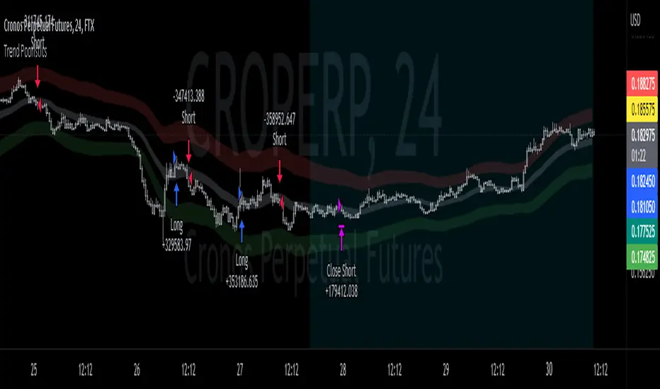
ICT OTE - Clean v6 (Indicator)ICT OTE — Indicator (Pine v6)
Comprehensive Guide & Rule-Based Trade Plan
This guide explains how to read and trade the Pine v6 indicator version of ICT’s Optimal Trade Entry (OTE). It covers chart elements, the 62–79% OTE zone (with 70.5% mid), confirmation logic, kill-zone gating, rule-based entries/stops/targets, and practical workflows.
1. Overview
The Optimal Trade Entry (OTE) is a core ICT concept that locates high-probability entries inside a Fibonacci retracement window between 62% and 79%, with 70.5% often used as a precise mid level. The indicator highlights that zone for the latest impulse (swing low to swing high for bullish, swing high to swing low for bearish), prints signal labels when price retraces into the box and a confirmation candle forms, and plots visual stop-loss and 1R/2R targets from your chosen entry line (62/70.5/79).
2. What the Indicator Draws
• OTE Box (62–79%): A green box for bullish OTE (drawn between 62% and 79% of the latest bullish impulse) and a red box for bearish OTE (drawn between 62% and 79% retracement of the latest bearish impulse).
• 70.5% Mid Line: A horizontal line through the OTE box at 70.5% (optional).
• Entry Line: Your selected entry reference: Top 62%, Mid 70.5%, or Bottom 79%.
• Signal Labels: ‘OTE Long’ appears when price touches the bullish OTE box and a confirmation candle prints; ‘OTE Short’ for the bearish side.
• Stop-Loss Guide: For longs: swing low of the dealing range; for shorts: swing high of the dealing range (visual plot).
• 1R/2R Target Lines: Two projected lines from the chosen entry to visualize 1R and 2R objectives (purely visual).
• Kill-Zone Shading (optional): Grey shading during London, NY-AM, and NY-PM windows, if gating is enabled.
3. Inputs & Settings
• Pivot Left/Right: Swing detection for impulses using pivot highs/lows (default 3/3).
• Draw OTE Box: Toggle drawing the 62–79% zone.
• Plot 70.5% Mid Line: Toggle the mid-line inside OTE.
• Entry Line: Choose the visual entry anchor (62% / 70.5% / 79%).
• Confirmation: Require a strong candle (default: close > open + continuation vs prior bar for longs; inverse for shorts).
• Stop/Targets: Toggle plotting the swing SL and 1R/2R targets.
• Kill-Zone Gating: If enabled, signals only fire in London (02:00–05:00 NY), NY-AM (08:00–11:00 NY), and NY-PM (13:00–15:00 NY).
• OTE Box Opacity: Adjust visual opacity of the box (default 85).
4. Rule-Based Entry Model
Use these steps exactly; do not skip.
1. Window: Optional — ensure you are inside an ICT kill-zone (London / NY-AM / NY-PM) if gating is enabled.
2. Impulse: Confirm the latest dealing range (pivot-based). Bullish = last swing low precedes last swing high; bearish = last swing high precedes last swing low.
3. OTE Box: Ensure price retraces into the 62–79% zone for the active impulse.
4. Confirmation: Wait for the required confirmation candle (strong or basic, per setting).
5. Entry Anchor: Use your selected line (62/70.5/79) as the reference for planning the fill.
6. Stops: Place SL at the swing extreme of the dealing range (longs: swing low; shorts: swing high).
7. Targets: Map 1R and 2R visual levels from the entry. Optionally prefer opposite liquidity or prior swing if closer (manual).
5. How to Read the Chart Step-by-Step
• Check background shading: are you inside a kill-zone (if enabled)?
• Identify the latest swing high/low markers (dealing range).
• Locate the OTE box for that impulse; confirm price retraced into the box.
• Inspect the confirmation candle: strong body and continuation (for longs: close > open AND close > prior high; for shorts: mirror).
• Use the entry line (62/70.5/79) as the reference; map SL and 1R/2R lines.
• If a signal label prints (‘OTE Long’ or ‘OTE Short’), you have alignment: timing, retracement, and confirmation.
6. Examples
Example Long (NY-AM): Price makes an impulse up (swing low then swing high). During NY-AM kill-zone, price retraces into the green OTE box. A strong bullish candle forms. Entry reference: 70.5% mid. SL at the swing low. Visual TP1/TP2 at 1R/2R.
Example Short (London): Price makes a bearish impulse (swing high then swing low). During London kill-zone, price retraces into the red OTE box. A strong bearish candle forms. Entry reference: 62%. SL at the swing high. Visual TP1/TP2 at 1R/2R.
7. Risk Management
• Fixed percent per trade: e.g., 1% risk relative to account equity (visual targets help sizing).
• One signal per kill-zone window: avoid overtrading inside the same hour.
• Respect invalidations: if a full body closes through the entire box or structure fails, stand down.
• Favor time/volatility windows for execution; avoid thin hours unless testing.
8. Common Pitfalls
• Forcing entries outside OTE: wait for a proper 62–79% retrace.
• Ignoring impulse definition: use confirmed pivots to avoid measuring from noise.
• Skipping confirmation: entries without a qualifying candle are lower quality.
• Inconsistent stops: SL belongs at the impulse extreme; avoid random micro-level stops.
• No timing discipline: kill-zone gating exists to filter low-probability periods.
9. Indicator Parameters — Quick Reference
• Pivot Left/Right: controls swing detection sensitivity (higher = stricter).
• Entry line: choose between 62%, 70.5%, and 79% for your signal anchor.
• Confirmation strength: toggle strong vs basic candle validation.
• Kill-zone gating: optional session-based signal filtering.
• Opacity/colors: cosmetic; adjust to your chart style.
10. Workflow Checklist
• Is the impulse correctly identified (pivot low/high order)?
• Is price inside the OTE box (62–79%)?
• Did the confirmation candle print?
• Is signal gating satisfied (if enabled)?
• Is SL mapped to the impulse extreme?
• Are 1R/2R levels clear from the entry?
• Any scheduled macro events in the window? (avoid surprise volatility).
11. References (ICT OTE & Kill-Zones)
• ICT Fibonacci / OTE levels: 62–79% with 70.5% mid — multiple tutorials and guides.
• ICT Kill-Zones: commonly used London / New York windows for timing entries.
