Dobrusky Pressure CoreWhat it does & who it’s for
Dobrusky Pressure Core is a volume by time replacement for traders who care about which side actually controls each bar. Instead of just plotting total volume, it splits each bar into estimated buy vs sell pressure and overlays a custom, session-aware volume baseline. It’s built for discretionary traders who want more nuanced volume context for entries, breakouts, and pullbacks.
Core ideas
Buy/sell pressure split: Each bar’s volume is broken into estimated buying and selling pressure.
Dominant side highlighting: The dominant side (buy or sell) is always displayed starting from the bottom of the bar, so you can quickly see who “owned” that bar.
Median-based baseline: Uses the median of the last N bars (50 by default) to build a robust volume baseline that’s less sensitive to one-off spikes.
Session-aware behavior: Baseline is calculated from Regular Trading Hours (RTH) by default, with an option to include Extended Hours (ETH) and a control to force Regular data on higher timeframes.
Volume regimes: Three multipliers (1x, 1.5x, 2x by default) show normal, high, and extreme volume regions.
Flexible display: Baseline can be shown as lines or as columns behind the volume, with full color customization.
How the pressure logic works
For each bar, the script:
Adjusts the range for gaps relative to the prior close so the “true” traded range is more consistent.
Computes buy pressure as a proportion of the adjusted range from low to close.
Defines sell pressure as: total volume minus buy pressure.
Marks the bar as buy-dominant if buy pressure ≥ sell pressure, otherwise sell-dominant, and colors the dominant side from the bottom to at least the midpoint using the selected buy/sell colors.
In practice, this turns basic volume columns into bars where the internal split and dominant side are clearly visible, helping you judge whether aggressive buyers or sellers truly controlled the bar instead of just looking at the price action.
Volume baseline & session logic
The script builds a session-aware baseline from recent volume:
Baseline length: A rolling window (default 50 bars) is used to compute a median volume value instead of a simple moving average.
RTH-only by default: By default, the baseline is built from Regular Trading Hours bars only. During extended hours, the baseline effectively “freezes” at the last RTH-derived value unless you choose to include extended session data.
Extended mode: If you select Extended mode, the script builds separate rolling baselines for RTH and ETH trading, using the appropriate one depending on the current session.
Force Regular Above Timeframe: On timeframes equal to or higher than your chosen threshold, the baseline automatically uses Regular session data, even if Extended is selected.
Multipliers: Three adjustable multipliers (1x, 1.5x, 2x by default) create normal, high, and extreme volume bands for quick identification.
This lets you choose whether you want a pure RTH reference or a baseline that adapts to extended-session activity.
Example ways to use it
1. Replace standard volume bars
Add Dobrusky Pressure Core to your volume pane and hide the default volume if you prefer a clean look.
Use the colors and split to see at a glance whether buyers or sellers were dominant on each bar.
2. Pressure confirmation for entries
For longs (example concept; adapt to your own rules):
Require that the entry bar’s buy pressure is greater than the previous bar’s sell pressure , or
If the entry and prior bar are both buy-dominant, require that the entry bar has more buy pressure than the prior bar.
This helps avoid taking a long when buying pressure is clearly fading relative to what sellers recently showed. A mirrored idea can be used for short setups with sell pressure.
3. Context from baseline multipliers
Use ~1x baseline as “normal” volume.
Watch for bars at or above 1.5x baseline when you want to see increased participation.
Treat 2x baseline and above as “extreme” volume zones that may mark climactic or especially important bars.
In practice, the baseline and multipliers are best used as context and filters, not as rigid rules.
Settings overview
Display
- Show Volume Baseline: toggle the baseline and its levels on or off.
- Baseline Display: choose between Line or Bars for the baseline visualization.
Baseline Calculation
- Length: lookback for the median baseline (default 50, configurable).
- Baseline Session Data: choose Regular or Extended to control which session data feeds the baseline.
Session Controls
- Regular Session (Local to TZ): define your RTH window (e.g., 0930-1600).
- Session Time Zone: choose the time zone used for that window.
- Force Regular Above Timeframe: on higher timeframes, force the baseline to use Regular session data only.
Baseline Levels
- Show Level x Multiplier 1/2/3: toggle each volume regime level.
- Multiplier 1/2/3: define what you consider normal, high, and extreme volume (defaults: 1.0, 1.5, 2.0).
Colors
- Buy Volume / Sell Volume: choose colors for buy and sell pressure.
- Baseline Bars (Base / x2 / x3): colors when the baseline is drawn as columns.
- Baseline Line (Base / x2 / x3): colors when the baseline is drawn as lines.
Limitations & best practices
This is a decision-support and visualization tool, not a buy/sell signal generator.
Best suited to markets where volume data is meaningful (e.g., index futures, liquid equities, liquid crypto).
The usefulness of any volume-based metric depends on the underlying data feed and instrument structure.
Always combine pressure and baseline context with your own strategy, risk management, and testing.
Originality
Most volume tools either show total volume only or compare it to a simple moving average. Dobrusky Pressure Core combines:
An intrabar buy/sell pressure split based on a gap-adjusted price range.
A median-based, configurable baseline built from session-specific data.
Session-aware behavior that keeps the baseline focused on Regular hours by default, with the option to incorporate Extended hours and force Regular data on higher timeframes.
The goal is to give traders a richer, session-aware view of participation and pressure that standard volume bars and simple SMA overlays don’t provide, while keeping everything transparent and open-source so users can review and adapt the logic.
Cari dalam skrip untuk "如何用wind搜索股票的发行价和份数"

Match Finder [theUltimator5]Match Finder is the dating app of indicators. It takes your current ticker and finds the most compatible match over a recent time period. The match may not be Mr. right, but it is Mr. right now. It doesn't forecast future connection, but it tells you current compatibility for today.
Jokes aside, it is a pattern–comparison tool that was designed to find the ticker that tracks most closely to the one you are currently looking at. It scans a user-defined list of 40 tickers (pre-set to a bunch of liquid ETFs) and finds which one most closely matches the recent price action of the current chart over a fixed lookback window.
LOGIC BEHIND THE SCENES
For each bar, the script:
Takes the last N bars (Correlation Window Length) of the current symbol.
Takes the last N bars of each selected comparison ticker.
Calculates the Pearson correlation between the current symbol and each comparison ticker.
Identifies the single best-matching ticker (highest positive correlation, excluding the current symbol itself).
Rescales and overlays that matched segment on the chart so you can visually compare shapes.
Optionally shows a correlation table with all tickers and their correlation values.
The use case of this indicator is to help you see which symbol has recently moved most similarly to your current chart, and how that shape looks when overlaid in the same panel. It helps you see which sectors it may be following most closely to.
Here is an image with arrows showing the elements of this indicator that will be mostly explained later.
USER INPUTS
1. Correlation Window Length
Default: 30
Range: 10–500
This is the number of bars used to compare the current symbol against each ticker.
Important - Larger values produce more “global” shape comparison but increase computational load and may cause the indicator to timeout if the length is too long
2. Drawing Mode
Options:
Scale Only - Adjusts min and max of the plotted line segment to match the chart over the range
Scale & Rotate - Scales as above, but matches the first and last point to the close of the chart over the range. This effectively rotates the pattern to force it to track the chart to an extent.
3. Show Correlation Table
When enabled (disabled by default), shows a table in the bottom-right of the chart that displays the correlation values over the lookback range for all 40 tickers. The best fit ticker is highlighted.
4. Best Fit Line Color
Color used to draw the overlaid best-match segment (yellow by default).
5. Ticker inputs (1–40)
Default set to a broad universe of major ETFs (e.g., SPY, QQQ, IWM, sector and bond ETFs, commodities, etc.).
You can replace these with any symbols supported by your data feed (stocks, ETFs, indexes, etc.).
The script always excludes the current chart’s symbol from being considered as its own best match.
NOTE: THIS INDICATOR IS EXTREMELY MEMORY INTENSIVE AND MAY TAKE SEVERAL SECONDS TO LOAD. PLEASE BE PATIENT AND GIVE THE INDICATOR UP TO 20 SECONDS FOR THE DATA TO DISPLAY

SMT + CVD (NQ vs ES) w/ AlertsSMT + CVD (NQ vs ES) w/ Alerts
This tool combines Smart Money Technique (SMT) and Cumulative Volume Delta (CVD) to highlight high-probability inflection points on NQ (primary) versus ES (secondary).
How it works
SMT condition: the primary breaks its most recent swing (High for bearish / Low for bullish) while the secondary does not break the corresponding swing within a small retest window.
CVD confirmation: at the same time, the primary’s CVD shows divergence (higher price but lower/equal CVD for shorts, lower price but higher/equal CVD for longs).
When both align, the script plots a marker/label and draws a line from the primary swing to the signal bar. Alerts are fired.
Signals & Alerts
Labels: “SMT+CVD DOWN/UP” on the signal bar.
Lines: connects the primary swing → signal bar so you can see the structure that produced the signal.
Alert names: “SMT+CVD Bearish” and “SMT+CVD Bullish.”
Inputs
Primary / Secondary symbols: defaults NQ & ES (you can change them).
Resolution: use chart timeframe or specify one.
Swing Left/Right Bars: pivot detection depth (higher = larger swings).
Break Window Bars: how many bars the secondary has to not break for SMT to be valid.
CVD Up/Down By: Close vs Previous Close (default) or Close vs Open.
Anchor CVD Daily: resets CVD at session/day start.
CVD Smoothing (EMA): smooths the CVD line (optional show).
FAST Pivots (no future bars): left-only swing detection so signals appear sooner and behave well in Replay/live.
Require Secondary Pivot: if ON, SMT checks wait for a confirmed secondary swing; if OFF, signals can appear while the secondary swing is still forming (useful for Replay/testing).
Show CVD line: optional, may compress price scale.
Non-repaint notes
With FAST Pivots ON, swings are detected with no future bars (minimal latency = leftBars).
With FAST Pivots OFF, standard pivots require rightBars future bars to confirm the swing (classic, but naturally delayed).
Tips
For intraday futures, keep leftBars/rightBars small (e.g., 3/3) and Break Window 1–3.
In Replay, enable FAST Pivots and consider disabling Require Secondary Pivot if you want signals to appear as soon as the primary breaks.
Combine with session filters, execution rules, or liquidity zones for context.

LibPvotLibrary "LibPvot"
This is a library for advanced technical analysis, specializing
in two core areas: the detection of price-oscillator
divergences and the analysis of market structure. It provides
a back-end engine for signal detection and a toolkit for
indicator plotting.
Key Features:
1. **Complete Divergence Suite (Class A, B, C):** The engine detects
all three major types of divergences, providing a full spectrum of
analytical signals:
- **Regular (A):** For potential trend reversals.
- **Hidden (B):** For potential trend continuations.
- **Exaggerated (C):** For identifying weakness at double tops/bottoms.
2. **Advanced Signal Filtering:** The detection logic uses a
percentage-based price tolerance (`prcTol`). This feature
enables the practical detection of Exaggerated divergences
(which rarely occur at the exact same price) and creates a
"dead zone" to filter insignificant noise from triggering
Regular divergences.
3. **Pivot Synchronization:** A bar tolerance (`barTol`) is used
to reliably match price and oscillator pivots that do not
align perfectly on the same bar, preventing missed signals.
4. **Signal Invalidation Logic:** Features two built-in invalidation
rules:
- An optional `invalidate` parameter automatically terminates
active divergences if the price or the oscillator breaks
the level of the confirming pivot.
- The engine also discards 'half-pivots' (e.g., a price pivot)
if a corresponding oscillator pivot does not appear within
the `barTol` window.
5. **Stateful Plotting Helpers:** Provides helper functions
(`bullDivPos` and `bearDivPos`) that abstract away the
state management issues of visualizing persistent signals.
They generate gap-free, accurately anchored data series
ready to be used in `plotshape` functions, simplifying
indicator-side code.
6. **Rich Data Output:** The core detection functions (`bullDiv`, `bearDiv`)
return a comprehensive 9-field data tuple. This includes the
boolean flags for each divergence type and the precise
coordinates (price, oscillator value, bar index) of both the
starting and the confirming pivots.
7. **Market Structure & Trend Analysis:** Includes a
`marketStructure` function to automatically identify pivot
highs/lows, classify their relationship (HH, LH, LL, HL),
detect structure breaks, and determine the current trend
state (Up, Down, Neutral) based on pivot sequences.
---
**DISCLAIMER**
This library is provided "AS IS" and for informational and
educational purposes only. It does not constitute financial,
investment, or trading advice.
The author assumes no liability for any errors, inaccuracies,
or omissions in the code. Using this library to build
trading indicators or strategies is entirely at your own risk.
As a developer using this library, you are solely responsible
for the rigorous testing, validation, and performance of any
scripts you create based on these functions. The author shall
not be held liable for any financial losses incurred directly
or indirectly from the use of this library or any scripts
derived from it.
bullDiv(priceSrc, oscSrc, leftLen, rightLen, depth, barTol, prcTol, persist, invalidate)
Detects bullish divergences (Regular, Hidden, Exaggerated) based on pivot lows.
Parameters:
priceSrc (float) : series float Price series to check for pivots (e.g., `low`).
oscSrc (float) : series float Oscillator series to check for pivots.
leftLen (int) : series int Number of bars to the left of a pivot (default 5).
rightLen (int) : series int Number of bars to the right of a pivot (default 5).
depth (int) : series int Maximum number of stored pivot pairs to check against (default 2).
barTol (int) : series int Maximum bar distance allowed between the price pivot and the oscillator pivot (default 3).
prcTol (float) : series float The percentage tolerance for comparing pivot prices. Used to detect Exaggerated
divergences and filter out market noise (default 0.05%).
persist (bool) : series bool If `true` (default), the divergence flag stays active for the entire duration of the signal.
If `false`, it returns a single-bar pulse on detection.
invalidate (bool) : series bool If `true` (default), terminates an active divergence if price or oscillator break
below the confirming pivot low.
Returns: A tuple containing comprehensive data for a detected bullish divergence.
regBull series bool `true` if a Regular bullish divergence (Class A) is active.
hidBull series bool `true` if a Hidden bullish divergence (Class B) is active.
exgBull series bool `true` if an Exaggerated bullish divergence (Class C) is active.
initPivotPrc series float Price value of the initial (older) pivot low.
initPivotOsz series float Oscillator value of the initial pivot low.
initPivotBar series int Bar index of the initial pivot low.
lastPivotPrc series float Price value of the last (confirming) pivot low.
lastPivotOsz series float Oscillator value of the last pivot low.
lastPivotBar series int Bar index of the last pivot low.
bearDiv(priceSrc, oscSrc, leftLen, rightLen, depth, barTol, prcTol, persist, invalidate)
Detects bearish divergences (Regular, Hidden, Exaggerated) based on pivot highs.
Parameters:
priceSrc (float) : series float Price series to check for pivots (e.g., `high`).
oscSrc (float) : series float Oscillator series to check for pivots.
leftLen (int) : series int Number of bars to the left of a pivot (default 5).
rightLen (int) : series int Number of bars to the right of a pivot (default 5).
depth (int) : series int Maximum number of stored pivot pairs to check against (default 2).
barTol (int) : series int Maximum bar distance allowed between the price pivot and the oscillator pivot (default 3).
prcTol (float) : series float The percentage tolerance for comparing pivot prices. Used to detect Exaggerated
divergences and filter out market noise (default 0.05%).
persist (bool) : series bool If `true` (default), the divergence flag stays active for the entire duration of the signal.
If `false`, it returns a single-bar pulse on detection.
invalidate (bool) : series bool If `true` (default), terminates an active divergence if price or oscillator break
above the confirming pivot high.
Returns: A tuple containing comprehensive data for a detected bearish divergence.
regBear series bool `true` if a Regular bearish divergence (Class A) is active.
hidBear series bool `true` if a Hidden bearish divergence (Class B) is active.
exgBear series bool `true` if an Exaggerated bearish divergence (Class C) is active.
initPivotPrc series float Price value of the initial (older) pivot high.
initPivotOsz series float Oscillator value of the initial pivot high.
initPivotBar series int Bar index of the initial pivot high.
lastPivotPrc series float Price value of the last (confirming) pivot high.
lastPivotOsz series float Oscillator value of the last pivot high.
lastPivotBar series int Bar index of the last pivot high.
bullDivPos(regBull, hidBull, exgBull, rightLen, yPos)
Calculates the plottable data series for bullish divergences. It manages
the complex state of a persistent signal's plotting window to ensure
gap-free and accurately anchored visualization.
Parameters:
regBull (bool) : series bool The regular bullish divergence flag from `bullDiv`.
hidBull (bool) : series bool The hidden bullish divergence flag from `bullDiv`.
exgBull (bool) : series bool The exaggerated bullish divergence flag from `bullDiv`.
rightLen (int) : series int The same `rightLen` value used in `bullDiv` for correct timing.
yPos (float) : series float The series providing the base Y-coordinate for the shapes (e.g., `low`).
Returns: A tuple of three `series float` for plotting bullish divergences.
regBullPosY series float Contains the static anchor Y-value for Regular divergences where a shape should be plotted; `na` otherwise.
hidBullPosY series float Contains the static anchor Y-value for Hidden divergences where a shape should be plotted; `na` otherwise.
exgBullPosY series float Contains the static anchor Y-value for Exaggerated divergences where a shape should be plotted; `na` otherwise.
bearDivPos(regBear, hidBear, exgBear, rightLen, yPos)
Calculates the plottable data series for bearish divergences. It manages
the complex state of a persistent signal's plotting window to ensure
gap-free and accurately anchored visualization.
Parameters:
regBear (bool) : series bool The regular bearish divergence flag from `bearDiv`.
hidBear (bool) : series bool The hidden bearish divergence flag from `bearDiv`.
exgBear (bool) : series bool The exaggerated bearish divergence flag from `bearDiv`.
rightLen (int) : series int The same `rightLen` value used in `bearDiv` for correct timing.
yPos (float) : series float The series providing the base Y-coordinate for the shapes (e.g., `high`).
Returns: A tuple of three `series float` for plotting bearish divergences.
regBearPosY series float Contains the static anchor Y-value for Regular divergences where a shape should be plotted; `na` otherwise.
hidBearPosY series float Contains the static anchor Y-value for Hidden divergences where a shape should be plotted; `na` otherwise.
exgBearPosY series float Contains the static anchor Y-value for Exaggerated divergences where a shape should be plotted; `na` otherwise.
marketStructure(highSrc, lowSrc, leftLen, rightLen, srcTol)
Analyzes the market structure by identifying pivot points, classifying
their sequence (e.g., Higher Highs, Lower Lows), and determining the
prevailing trend state.
Parameters:
highSrc (float) : series float Price series for pivot high detection (e.g., `high`).
lowSrc (float) : series float Price series for pivot low detection (e.g., `low`).
leftLen (int) : series int Number of bars to the left of a pivot (default 5).
rightLen (int) : series int Number of bars to the right of a pivot (default 5).
srcTol (float) : series float Percentage tolerance to consider two pivots as 'equal' (default 0.05%).
Returns: A tuple containing detailed market structure information.
pivType series PivType The type of the most recently formed pivot (e.g., `hh`, `ll`).
lastPivHi series float The price level of the last confirmed pivot high.
lastPivLo series float The price level of the last confirmed pivot low.
lastPiv series float The price level of the last confirmed pivot (either high or low).
pivHiBroken series bool `true` if the price has broken above the last pivot high.
pivLoBroken series bool `true` if the price has broken below the last pivot low.
trendState series TrendState The current trend state (`up`, `down`, or `neutral`).

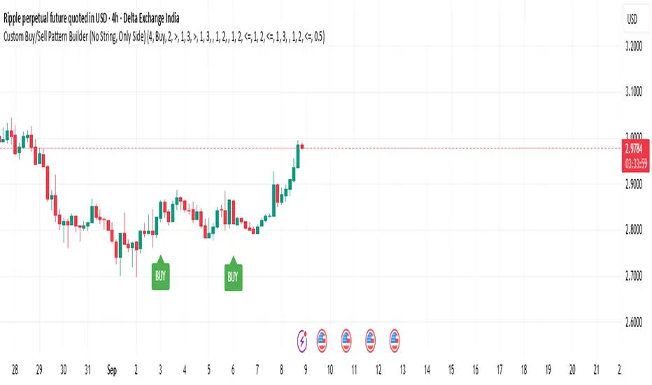
London Breakout Structure by Ale 2This indicator identifies market structure breakouts (CHOCH/BOS) within a specific London session window, highlighting potential breakout trades with automatic entry, stop loss (SL), and take profit (TP) levels.
It helps traders focus on high-probability breakouts when volatility increases after the Asian session, using price structure, ATR-based volatility filters, and a custom risk/reward setup.
🔹 Example of Strategy Application
Define your session (e.g. 04:00 to 05:00).
Wait for a CHOCH (Change of Character) inside this session.
If a bullish CHOCH occurs → go LONG at candle close.
If a bearish CHOCH occurs → go SHORT at candle close.
SL is set below/above the previous swing using ATR × multiplier.
TP is calculated automatically based on your R:R ratio.
📊 Example:
When price breaks above the last swing high within the session, a “BUY” label appears and the indicator draws Entry, SL, and TP levels automatically.
If the breakout fails and price closes below the opposite structure, a “SELL” signal will replace the bullish setup.
🔹 Details
The logic is based on structural shifts (CHOCH/BOS):
A CHOCH occurs when price breaks and closes beyond the most recent high/low.
The indicator dynamically detects these shifts in structure, validating them only inside your chosen time window (e.g. the London Open).
The ATR filter ensures setups are valid only when the range has enough volatility, avoiding false signals in low-volume hours.
You can also visualize:
The session area (purple background)
Entry, Stop Loss, and Take Profit levels
Direction labels (BUY/SELL)
ATR line for volatility context
🔹 Configuration
Start / End Hour: define your preferred trading window.
ATR Length & Multiplier: adjust for volatility.
Risk/Reward Ratio: set your desired R:R (default 1:2).
Minimum Range Filter: avoids signals with tight SLs.
Alerts: receive notifications when breakout conditions occur.
🔹 Recommendations
Works best on 15m or 5m charts during London session.
Designed for breakout and structure-based traders.
Works on Forex, Crypto, and Indices.
Ideal as a visual and educational tool for understanding BOS/CHOCH behavior.

USD Session 8FX - LDN & NY (TF-invariant, Live + Table)What it is
A USD strength/weakness meter for the London (08:00–08:45) or New York (15:30–16:00/16:15) session. It blends the movement of 8 markets—EURUSD, GBPUSD, AUDUSD, NZDUSD, USDCHF, USDCAD, USDJPY, XAUUSD—into one Score that is timeframe-invariant (it uses a 1-minute “boundary TF” under the hood so changing chart TF doesn’t change the math).
Core logic (simple)
During the chosen session window, it records each symbol’s start and live end prices, computes returns, optionally normalizes by ATR (volatility), applies your weights, and averages anti-USD (EUR/GBP/AUD/NZD/XAU) vs USD-base (CHF/CAD/JPY) groups.
The final Score is the normalized sum of weighted contributions:
Score > 0 → “USD Strong”
Score < 0 → “USD Weak”
At the session close it freezes (“Locked”) the results so you can review them later.
What you see
Main plot: the USD Score line (with a 0 baseline).
Optional lines: Anti-USD average vs USD-base average (post-normalization, pre-weights).
Session background shading (London silver, New York aqua).
Live table with:
Each symbol’s % change, its weight, and its contribution to the Score.
TOP badges for the two biggest drivers (by absolute contribution).
A Side column (only for the two TOPs) showing BUY/SELL aligned with the USD verdict (e.g., if USD Strong → SELL anti-USD pairs like EURUSD, BUY USD-base like USDCHF).
Verdict row with USD Strong/Weak, the Score value, the window text, and whether you’re LIVE / CLOSED / FROZEN.
Trade Gate panel:
Shows Verdict (USD Strong/Weak), Bias OK/weak (|Score| vs your threshold), Top-1/Top-2 VWAP checks, an overall GATE: OK/NO, and an Entry hint string (e.g., “SELL EURUSD, BUY USDCHF”) when conditions align.
VWAP “Trade Gate”
It confirms alignment between the USD bias and price vs VWAP for the top movers:
If USD Strong: anti-USD symbols should be below VWAP (short bias), USD-base symbols above VWAP (long bias).
If USD Weak: the opposite.
Gate = OK only if |Score| ≥ minAbsScore and at least one of the two TOP symbols is on the correct side of VWAP.
Tip: set vwapTF to an intraday value (“1”, “5”, “15”) for reliable VWAP on higher-TF charts.
Alerts
At session close: “USD Strong/Weak – session close”.
Live threshold: alerts when |Score| crosses your intraday threshold up/down.
Entry hint (Gate OK): triggers when the Gate flips from NO → OK inside the window.
If you create an alert of type “Any alert() function call”, you also get a dynamic message like:
ENTRY HINT • Hint: SELL EURUSD, BUY USDCHF
Key inputs you can tweak
Session: London vs New York; NY end time 16:00 or 16:15.
Timezone: default Europe/Tirane.
Boundary TF: default “1” (keeps the indicator TF-invariant).
minAbsScore: sensitivity threshold for “Bias OK”.
ATR normalization (len): stabilizes comparisons across different volatility regimes.
VWAP settings: toggle panel and set vwapTF.
How to use (playbook)
Choose the session (e.g., New York 15:30–16:15), keep Boundary TF = 1.
If you’re on a higher-TF chart, set vwapTF = "1" or "5".
Watch Score and Verdict; when |Score| ≥ minAbsScore, bias is meaningful.
Check Top-1/Top-2 and the Trade Gate:
If Gate = OK, use the Entry hint (e.g., “SELL EURUSD, BUY USDCHF”) as the aligned idea.
Use your own execution rules (e.g., structure, risk, stops) on the suggested symbols.
After close, review the Frozen table to validate behavior and refine thresholds/weights.
Notes & edge cases
If some markets are illiquid/holiday, a few returns may be na; the script handles that gracefully.
If ta.vwap is na on high TFs, the Gate will simply not confirm—set vwapTF intraday.
You can customize weights (e.g., reduce XAUUSD to -0.3 or similar) to suit your basket philosophy.
If you want, I can add toggles to show Side for all 8 symbols, or print a one-line summary (e.g., “USD Strong • Score 0.23 • Gate OK • SELL EURUSD, BUY USDCHF”) in the top-left of the pane.

Trading Activity Index (Zeiierman)█ Overview
Trading Activity Index (Zeiierman) is a volume-based market activity meter that transforms dollar-volume into a smooth, normalized “activity index.”
It highlights when market participation is unusually low or high with a dynamic color gradient:
Light Blue → Low Activity (thin participation, low liquidity conditions)
Red/Orange → High Activity (active markets, large trades flowing in)
Additional percentile bands (20/40/60/80%) give context, helping you see whether the current activity level is in the bottom quintile, mid-range, or near historical extremes.
█ How It Works
⚪ Dollar Volume Transformation
Each bar, dollar volume is computed:
float dlrVol = close * volume
float dlrVolAvg = ta.sma(dlrVol, len_form)
Dollar volume = price × volume, smoothed by a configurable SMA window.
The result is log-transformed, compressing large outliers for a more stable signal.
⚪ Rolling Percentiles & Ranking
The log-dollar-volume series is compared to its rolling history (len_hist bars):
float p20 = ta.percentile_linear_interpolation(vscale, len_hist, 20)
float p40 = ta.percentile_linear_interpolation(vscale, len_hist, 40)
float p60 = ta.percentile_linear_interpolation(vscale, len_hist, 60)
float p80 = ta.percentile_linear_interpolation(vscale, len_hist, 80)
A normalized rank (0–1) is produced to color the main Trading Activity line.
█ How to Use
⚪ Detect High-Impact Sessions
Quickly see if today’s session is active or quiet relative to its own history — great for filtering setups that need activity.
⚪ Spot Breakouts & Traps
Combine with price action:
High activity near breakouts = strong follow-through likely.
Low activity breakouts = vulnerable to fake-outs.
⚪ Market Regime Context
Percentile bands help you assess whether participation is building up, in the middle of the range, or drying out — valuable for timing mean-reversion trades.
Above 80th percentile (red/orange) → Market is highly active, breakout trades and trend strategies are favored.
Below 20th percentile (light blue) → Market is quiet; fade moves or wait for expansion.
Watch transitions from blue → orange as a signal of growing institutional participation.
█ Settings
Formation Window (bars) – Number of bars used to average dollar volume before log transform.
History Window (bars) – Lookback period for percentile calculations and rank normalization.
-----------------
Disclaimer
The content provided in my scripts, indicators, ideas, algorithms, and systems is for educational and informational purposes only. It does not constitute financial advice, investment recommendations, or a solicitation to buy or sell any financial instruments. I will not accept liability for any loss or damage, including without limitation any loss of profit, which may arise directly or indirectly from the use of or reliance on such information.
All investments involve risk, and the past performance of a security, industry, sector, market, financial product, trading strategy, backtest, or individual's trading does not guarantee future results or returns. Investors are fully responsible for any investment decisions they make. Such decisions should be based solely on an evaluation of their financial circumstances, investment objectives, risk tolerance, and liquidity needs.

Custom Buy/Sell Pattern BuilderAre you tired of using trading indicators that only let you follow fixed, pre-designed rules? Do you wish you could build your own “Buy” or “Sell” signals, experiment with your own ideas, or see instantly if your unique pattern works—without learning coding or hiring a developer?
The Custom Buy/Sell Pattern Builder is designed for YOU.
This TradingView indicator lets ANY trader—even a complete beginner—define exactly what kind of price and volume conditions should create a BUY or SELL label on any chart, in any market, at any timeframe.
You don’t need to know programming. You don’t need to know the definition of a hammer, doji, volume spike, or Engulfing pattern.
With a few clicks and easy dropdown choices, you can:
Make your own rules for buying or selling
Choose how many candles your pattern should look at
Decide if you want the biggest body, the lowest volume, the biggest movement, or any combination you can imagine
The result?
You’ll see clear “BUY” or “SELL” labels automatically show up on your chart whenever the exact rule YOU built matches current price action.
No more guessing. No more forced strategies. Just pure control and visual feedback!
Why Is This Powerful?
Traditional indicators (like MACD, RSI, or even classic candlestick scanners) work the same for everyone—and only as their inventors defined.
But every trader, and every market, is unique.
What if you could say:
“Show me a ‘SELL’ every time the newest candle is bigger than the one before, but with LESS volume, while the bar before that had an even smaller body—but more volume than all others?”
With this tool, it’s EASY!
You simply pick which candle you want to compare (most recent, previous, etc), what to compare (body or volume—body means the candle’s “thickness”, from open to close), choose “greater than”, “less than”, or “equal to”, and set a multiplier if you want (like “half as much”, “twice as big”, etc).
After this, if any bar on the chart fits all your rules, it will mark it as a BUY or SELL, depending on your selection.
This means—
Beginners can start experimenting with their intuition or small ideas, without tech hurdles
Experienced traders can visualize and fine-tune any possible logic, before they commit to backtesting or automating a real strategy
Every “what if” or “I wonder” setup is just 2–3 clicks away
How Does It Work? Simple Steps
1. Choose Your Signal Type
“Buy” or “Sell”
This tells the indicator whether to mark the qualifying bars with a green “BUY” or red “SELL” label
2. Pick How Many Candles To Use
“Pattern Candle Count” input (2, 3, or 4)
Example: If you use 4, the pattern will be applied to the most recent 4 candles at every step
3. Define Your Pattern With Inputs
For each candle (from newest “0” to oldest “3”), you can set:
Body Condition (example: “is this candle’s body bigger/smaller/equal to another?”)
Pick which candle to compare against
Pick “>”, “<”, “>=”, “<=”, or “=”
Set a multiplier if needed (like “0.5” to mean “half as big as” or “2” for “twice as big as”)
Volume Condition (exact same choices, but based on trading volume—not the candle’s price body)
For example:
“Candle0 Body > Candle2 Body”
means “the latest candle’s real-body (open–close) is bigger than the one two bars ago.”
“Candle1 Volume <= Candle2 Volume”
means “the previous candle’s volume is less than or equal to the volume of the bar two periods ago.”
You can leave a comparison blank if you don’t want to use it for a particular candle.
What Happens After You Set Your Rules?
Every bar on your chart is checked for your logic:
If ALL body AND volume conditions are true (for each candle you specified),
AND
The signal side (“Buy” or “Sell”) matches your dropdown,
Then a green “BUY” or red “SELL” label will show right on the bar, so you can visually spot exactly where your logic works!
Practical Example:
Suppose you want an entry setup that is:
“Sell whenever the newest candle’s body is bigger than two bars ago, body before that is bigger than three bars ago, AND the newest candle’s volume is less than or equal to two bars ago, AND the candle three bars ago’s volume is less than or equal to half the candle two bars ago’s volume.”
You’d set:
Pattern Candle Count: 4
Side: Sell
Candle0 Body Ref#: 2, Op: >, Mult: 1
Candle1 Body Ref#: 3, Op: >, Mult: 1
Candle0 Vol Ref#: 2, Op: <=, Mult: 1
Candle3 Vol Ref#: 2, Op: <=, Mult: 0.5
And the script will find all “SELL” bars on your chart matching these conditions.
Inputs Section: What Does Each Setting Do?
Let’s break down each input in the indicator’s Settings one by one, so even if you’re new, you’ll understand exactly how to use it!
1. Pattern Candle Count (2–4)
What is it?
This sets how many candles in a row you want your rule to look at.
Example:
“4” means your rules are based on the most recent candle and the 3 before it.
“2” means you are only comparing the current and previous candles.
Tip:
Beginners often use 4 to spot stronger patterns, but you can experiment!
2. Signal Side
What is it?
Choose “Buy” or “Sell”. The word you pick here decides which colored label (green for Buy, red for Sell) appears if your pattern matches.
Example:
Want to spot where “Sell” is likely? Pick “Sell”.
Change to “Buy” if you want bullish signals instead.
3. Body & Volume Comparison Settings (per Candle)
For each candle (#0 is newest/current, #3 is oldest in your pattern window):
Body Comparison
Candle# Body Ref#
Choose which other candle you want to compare this one’s body to.
“0” = newest, “1” = previous, “2” = two bars ago, “3” = three bars ago
Candle# Body Op (Operator; >, <, >=, <=, =)
How do you want to compare?
“>” means “greater than” (is bigger than)
“<” means “less than” (is smaller than)
“=” means “equal to”
Candle# Body Mult (Multiplier)
If you want relative comparisons. For example, with Mult=1:
“Candle0 body > Candle2 body x 1” means just “0 is larger than 2.”
“Candle0 body > Candle2 body x 2” means “0 is more than double 2.”
Volume Comparison
Candle# Vol Ref# / Op / Mult
Exact same logic as body, but works on the “Volume” of each candle (how much was traded during that bar).
How to Set Up a Rule (Step by Step Example)
Say you want to mark a Sell every time:
The most recent candle’s real body is BIGGER than the candle 2 bars ago;
The previous candle’s body is also BIGGER than the candle 3 bars ago;
The current candle’s volume is LESS than or equal to the volume of candle 2;
The previous candle’s volume is LESS than or equal to candle 2’s volume;
The candle 3 bars ago’s volume is LESS than or equal to HALF candle 2’s volume.
You’d set:
Pattern Candle Count: 4
Side: "Sell"
Candle0 Body Ref#: 2, Op: “>”, Mult: 1
Candle1 Body Ref#: 3, Op: “>”, Mult: 1
Candle0 Vol Ref#: 2, Op: “<=”, Mult: 1
Candle1 Vol Ref#: 2, Op: “<=”, Mult: 1
Candle3 Vol Ref#: 2, Op: “<=”, Mult: 0.5
All other comparisons (operators) can be left blank if you don’t want to use them!
When these rules are met, a bright red “SELL” label will appear right above the bar matching all your conditions.
Practical Tips & FAQ for Beginners
What does “body” mean?
It’s the “true range” of the candle: the difference between open and close. This ignores wicks for simple setups.
What does “volume” mean?
This is the total trading activity during that candle/bar. Many traders believe that patterns with different volume “meaning” (such as low-volume up bars, or high-volume down bars) signal a meaningful change.
What if nothing shows on chart?
It just means your current rules are rarely or never matched! Try making your comparisons simpler (maybe just 2-body and 2-volume conditions to start).
You can always hit “Reset Settings” to go back to default.
Can I use this for both buying and selling?
YES! You can detect both bullish (Buy) and bearish (Sell) custom conditions; just switch “Signal Side.”
Do I need to know coding?
Not at all! Everything is in simple input panels.
Creative Use Cases, Example Recipes & Troubleshooting
Creative Ways to Use
Spotting Reversals
Example:
Buy when: the newest candle body is LARGER than the previous 3 bars, but ALL volumes are lower than their neighbors.
Why? Sometimes, a big candle with surprisingly low volume after a sequence of small bars can signal a reversal.
Finding Exhaustion Moves
Example:
Sell when: the current bar body is twice as big as two bars ago, but volume is half.
Why? A very big candle with very little volume compared to similar bars may show the move is “running out of steam.”
Custom “Breakout + Confirmation” Patterns
Example:
Buy when:
Candle 0’s body is greater than Candle 2’s by at least 1.5x,
Candle 0’s volume is greater than Candle 1 and Candle 2,
Candle 1’s volume is less than Candle 0.
Why? This could catch strong breakouts but filter out noisy moves.
Multi-bar Bias/Squeeze Filter
Use “Pattern Candle Count: 4”
Set all 4 volume conditions to “<” and each reference to the previous candle.
Now, a BUY or SELL only marks when each bar is “dryer”/less active than the last — a classic squeeze or low-volatility buildup.
Troubleshooting Guide
“I don’t see any Buy/Sell label; is something broken?”
Most likely, your rules are too strict or rare! Try using only two comparisons and leave other “Op” inputs blank as a test.
Double-check you have enough candles on the chart: you need at least as many bars as your pattern count.
“Why does a label appear but not where I expect?”
Remember, the script checks your rules for every NEW candle. The candle “0” is always the most recent, then “1” is one bar back, etc.
Check the color and type chosen: “Signal Side” must be “Buy” for green, “Sell” for red.
“What if I want a more complex pattern?”
Stack conditions! You can demand the body/volume of each candle in your window meet a different rule or all follow the same rule in sequence.
Mini Glossary — For Newcomers
Candle/Bar: Each bar on the chart, shows price movement during a fixed time (e.g., one minute, one hour, one day).
Body: The colored (or filled) part of the candle — the open-to-close price range.
Volume: How much of the asset was actually traded that candle/bar.
Reference Index: When you pick “2” as a reference, it means “the candle two bars ago in the pattern window.”
Operator (“Op”): The math symbol used to compare (>, <, =, etc).
Signal Side: Whether you want to highlight bullish (“Buy”) or bearish (“Sell”) bars.
Tips for Getting More Value
Start Simple—try just one or two conditions at first. See what lights up. Slowly add more logic as you get comfortable.
Watch the chart live as you change settings. The labels update instantly—this makes strategy design fast and visual!
Try flipping your ideas: If a certain pattern doesn’t work for buys, try reversing the direction for possible “sell” setups.
Remember: There is NO wrong idea. This indicator is only limited by your creativity—it’s a “strategy playground.”
Example Quick-Start Recipes
Classic Sell:
4 candles, side = Sell
Candle0 Body > Candle2; Candle1 Body > Candle3
Candle0 Vol <= Candle2; Candle1 Vol <= Candle2; Candle3 Vol <= Candle2 × 0.5
Simple Buy After Pause:
3 candles, side = Buy
Candle0 Body > Candle1; Candle0 Vol > Candle1
All other Ops blank
Low-Volume Pullback for Entry:
4 candles, side = Buy
Candle0 Body > Candle2
Candle0 Vol < Candle1; Candle1 Vol < Candle2; Candle2 Vol < Candle3
Final Words
Think of this as your “pattern lab.” No code, no guesswork—just experiment, see what the market actually gives, and design your own visual rulebook.
If you’re stuck, reset the script to defaults—it’s always safe to start again!
If you want more ready-made “recipes” for different strategies/styles, just ask and I’ll send some more setups for you.
Happy building—and may your edge always be YOUR edge!
Order Blocks + Order-Flow ProxiesOrder Blocks + Order-Flow Proxies
This indicator combines structural analysis of order blocks with lightweight order-flow style proxies, providing a tool for chart annotation and contextual study. It is designed to help users visualize where significant structural shifts occur and how simple volume-based signals behave around those areas. The script does not guarantee profitable outcomes, nor does it issue financial advice. It is intended purely for research, learning, and discretionary use.
Conceptual Background
Order Blocks
An “order block” is a term often used to describe a zone on the chart where price left behind a significant reversal or imbalance before continuing strongly in the opposite direction. In practice, this can mean the last bullish or bearish candle before a strong breakout. Traders sometimes study these regions because they believe that unfilled resting orders may exist there, or simply because they mark important pivots in price structure. This indicator detects such moments by scanning for breaks of structure (BOS). When price pushes above or below recent swing levels with sufficient displacement, the script identifies the prior opposite candle as the potential order block.
Break of Structure
A break of structure in this context is defined when the closing price moves beyond the highest high or lowest low of a short lookback window. The script compares the magnitude of this break to an ATR-based displacement filter. This helps ensure that only meaningful moves are marked rather than small, random fluctuations.
Order-Flow Proxies
Traditional order flow analysis may use bid/ask data, footprint charts, or volume profiles. Because TradingView scripts cannot access true order-book data, this indicator instead uses proxy signals derived from standard chart data:
Delta (proxy): Estimated imbalance of buying vs. selling pressure, approximated using bar direction and volume.
Imbalance ratio: Normalizes delta by total volume, ranging between -1 and +1 in theory.
Cumulative Delta (CVD): Running sum of delta over time.
Effort vs. Result (EvR): A comparison between volume and actual bar movement, highlighting cases where large effort produced little result (or vice versa).
These are not real order-flow measurements, but rather simple mathematical constructs that mimic some of its logic.
How the Script Works
Detecting Break of Structure
The user specifies a swing length. When price closes above the recent high (for bullish BOS) or below the recent low (for bearish BOS), a potential shift is recorded.
To qualify, the breakout must exceed a displacement filter proportional to the ATR. This helps filter out weak moves.
Locating the Order Block Candle
Once a BOS is confirmed, the script looks back within a short window to find the last opposite-colored candle.
The high/low or open/close of that candle (depending on user settings) is marked as the potential order block zone.
Drawing and Maintaining Zones
Each order block is represented as a colored rectangle extending forward in time.
Bullish zones are teal by default, bearish zones are red.
Zones extend until invalidated (price closing or wicking beyond them, depending on user preference) or until a user-defined lifespan expires.
A pruning mechanism ensures that only the most recent set number of zones remain, preventing chart overload.
Monitoring Touches
The script checks whether the current bar’s range overlaps any existing order block.
If so, the “closest” zone is considered touched, and a label may appear on the chart.
Confirmation Filters
Touches can optionally be confirmed by order-flow proxies.
For a bullish confirmation, the following must align:
Imbalance ratio above threshold,
Delta EMA positive,
Effort vs. Result positive.
For a bearish confirmation, the opposite holds true.
Optionally, a higher-timeframe EMA slope filter can gate these confirmations. For example, a bullish confirmation may only be accepted if the higher-timeframe EMA is sloping upward.
Alerts
Users may create alerts based on conditions such as “bullish touch confirmed” or “bearish touch confirmed.”
Alerts can be gated to only fire after bar close, reducing intrabar noise.
Standard alertcondition calls are provided, and optional inline alert() calls can be enabled.
Inputs and Customization
Structure & OB
Swing length: Defines how many bars back to check for BOS.
ATR length & displacement factor: Adjust sensitivity for structural breaks.
Body vs. wick reference: Choose whether zones are based on candle bodies or full ranges.
Invalidation rule: Pick between wick breach or close beyond the level.
Lifespan (bars): Limit how long a zone remains active.
Max keep: Cap the number of zones stored to reduce clutter.
Order-Flow Proxies
Delta mode: Choose between “Close vs Previous Close” or “Body” for delta calculation.
EMA length: Smooths the delta/imbalance series.
Z-score lookback: Defines the averaging window for EvR.
Confirmation thresholds: Adjust the imbalance levels required for long/short confirmation.
Higher Timeframe Filter
Enable HTF gate: Optional filter requiring higher-timeframe EMA slope alignment.
HTF timeframe & EMA length: Configurable for context alignment.
Style
Colors and transparency for bullish and bearish zones.
Border color customization.
Alerts
Enable inline alerts: Optional direct calls to alert().
Alerts on bar close only: Helps avoid multiple firings during bar formation.
Practical Use
This tool is best seen as a way to annotate charts and to study how simple volume-derived signals behave near important structural levels. Some users may:
Observe whether order blocks line up with later price reactions.
Study how imbalance or cumulative delta conditions align with these zones.
Use it in a discretionary workflow to highlight areas of interest for deeper analysis.
Because the proxies are based only on candle OHLCV data, they are approximations. They cannot replace true depth-of-market analysis. Similarly, order block detection here is one specific algorithmic interpretation; other traders may define order blocks differently.
Limitations and Disclaimers
This indicator does not predict future price movement.
It does not access real order book or tick-by-tick data. All signals are derived from bar OHLCV.
Past performance of signals or zones does not guarantee future results.
The script is for educational and informational purposes only. It is not financial advice.
Users should test thoroughly, adjust parameters to their own instruments and timeframes, and use it in combination with broader analysis.
Summary
The Order Blocks + Order-Flow Proxies script is an experimental study tool that:
Detects potential order blocks using a displacement-filtered break of structure.
Marks these zones as boxes that persist until invalidation or expiry.
Provides lightweight order-flow-style proxies such as delta, imbalance, CVD, and effort vs. result.
Allows confirmation of zone touches through these proxies and optional higher-timeframe context.
Offers flexible customization, alerting, and chart-style options.
It is not a trading system by itself but rather a framework for studying price/volume behavior around structurally significant areas. With careful exploration, it can give users new ways to visualize market structure and to understand how simple flow-like measures behave in those contexts.

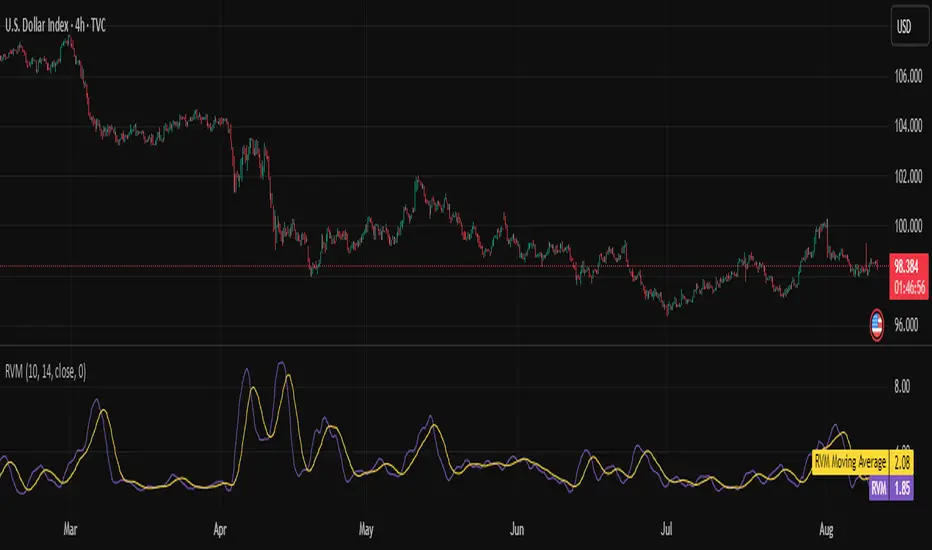
Relative Volatility Mass [SciQua]The ⚖️ Relative Volatility Mass (RVM) is a volatility-based tool inspired by the Relative Volatility Index (RVI) .
While the RVI measures the ratio of upward to downward volatility over a period, RVM takes a different approach:
It sums the standard deviation of price changes over a rolling window, separating upward volatility from downward volatility .
The result is a measure of the total “volatility mass” over a user-defined period, rather than an average or normalized ratio.
This makes RVM particularly useful for identifying sustained high-volatility conditions without being diluted by averaging.
────────────────────────────────────────────────────────────
╭────────────╮
How It Works
╰────────────╯
1. Standard Deviation Calculation
• Computes the standard deviation of the chosen `Source` over a `Standard Deviation Length` (`stdDevLen`).
2. Directional Separation
• Volatility on up bars (`chg > 0`) is treated as upward volatility .
• Volatility on down bars (`chg < 0`) is treated as downward volatility .
3. Rolling Sum
• Over a `Sum Length` (`sumLen`), the upward and downward volatilities are summed separately using `math.sum()`.
4. Relative Volatility Mass
• The two sums are added together to get the total volatility mass for the rolling window.
Formula:
RVM = Σ(σ up) + Σ(σ down)
where σ is the standard deviation over `stdDevLen`.
╭────────────╮
Key Features
╰────────────╯
Directional Volatility Tracking – Differentiates between volatility during price advances vs. declines.
Rolling Volatility Mass – Shows the total standard deviation accumulation over a given period.
Optional Smoothing – Multiple MA types, including SMA, EMA, SMMA (RMA), WMA, VWMA.
Bollinger Band Overlay – Available when SMA is selected, with adjustable standard deviation multiplier.
Configurable Source – Apply RVM to `close`, `open`, `hl2`, or any custom source.
╭─────╮
Usage
╰─────╯
Trend Confirmation: High RVM values can confirm strong trending conditions.
Breakout Detection: Spikes in RVM often precede or accompany price breakouts.
Volatility Cycle Analysis: Compare periods of contraction and expansion.
RVM is not bounded like the RVI, so absolute values depend on market volatility and chosen parameters.
Consider normalizing or using smoothing for easier visual comparison.
╭────────────────╮
Example Settings
╰────────────────╯
Short-term volatility detection: `stdDevLen = 5`, `sumLen = 10`
Medium-term trend volatility: `stdDevLen = 14`, `sumLen = 20`
Enable `SMA + Bollinger Bands` to visualize when volatility is unusually high or low relative to recent history.
╭───────────────────╮
Notes & Limitations
╰───────────────────╯
Not a directional signal by itself — use alongside price structure, volume, or other indicators.
Higher `sumLen` will smooth short-term fluctuations but reduce responsiveness.
Because it sums, not averages, values will scale with both volatility and chosen window size.
╭───────╮
Credits
╰───────╯
Based on the Relative Volatility Index concept by Donald Dorsey (1993).
TradingView
SciQua - Joshua Danford
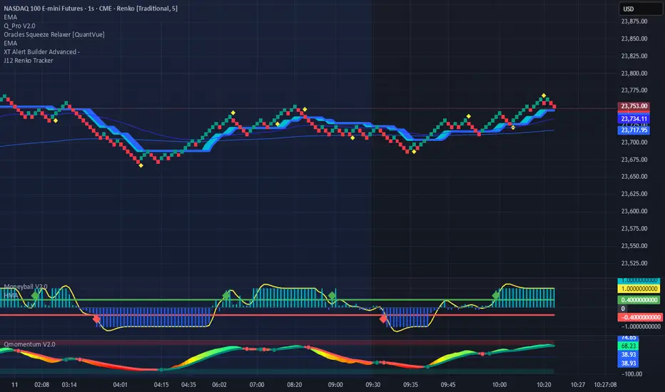
Renko Price TrackerRenko Sequential Signal – qLine + Moneyball Confirmation
This indicator is designed for Renko chart traders who want to combine price action relative to a key line (qLine) with Moneyball buy/sell signals as a confirmation. It helps filter trades so you only get signals when both conditions align within a chosen time window.
How It Works
First Event – Price Trigger
Detects when the Renko close crosses above/below your selected qLine plot from the qPro indicator.
You can choose between:
Cross – only triggers on an actual crossover/crossunder.
State (Close) – triggers whenever price closes above/below qLine.
Second Event – Moneyball Confirmation
Waits for Moneyball’s Buy Signal (for long) or Bear/Sell Signal (for short) plot to fire.
You select the exact Moneyball plot from the source menu.
You can specify how the Moneyball signal is interpreted (== 1, >= 1, or any nonzero value).
Sequential Logic
The Moneyball signal must occur within N Renko bricks after the price event.
The final buy/sell signal is printed on the Moneyball bar.
Key Features
Works natively on Renko charts.
Adjustable confirmation window (0–5 bricks).
Flexible detection for both qLine and Moneyball signals.
Customizable label sizes, arrow display, and alerts.
Alerts fire for both buy and sell conditions:
BUY: qLine ➜ Moneyball Buy
SELL: qLine ➜ Moneyball Sell
Inputs
qLine Source – Pick the qPro qLine plot.
Price Event Type – Cross or State.
Moneyball Buy/Sell Signal Plots – Select the correct plots from your Moneyball indicator.
Confirmation Window – Bars allowed between events.
Visual Settings – Label size, arrow visibility, etc.
Use Case
Ideal for traders who:
Want a double-confirmation entry system.
Use Renko charts for cleaner trend detection.
Already have qPro and Moneyball loaded, but want an automated, rule-based confluence check.
Fibonacci Sequence Moving Average [BackQuant]Fibonacci Sequence Moving Average with Adaptive Oscillator
1. Overview
The Fibonacci Sequence Moving Average indicator is a two‑part trading framework that combines a custom moving average built from the famous Fibonacci number set with a fully featured oscillator, normalisation engine and divergence suite. The moving average half delivers an adaptive trend line that respects natural market rhythms, while the oscillator half translates that trend information into a bounded momentum stream that is easy to read, easy to compare across assets and rich in confluence signals. Everything from weighting logic to colour palettes can be customised, so the tool comfortably fits scalpers zooming into one‑minute candles as well as position traders running multi‑month trend following campaigns.
2. Core Calculation
Fibonacci periods – The default length array is 5, 8, 13, 21, 34. A single multiplier input lets you scale the whole family up or down without breaking the golden‑ratio spacing. For example a multiplier of 3 yields 15, 24, 39, 63, 102.
Component averages – Each period is passed through Simple Moving Average logic to produce five baseline curves (ma1 through ma5).
Weighting methods – You decide how those five values are blended:
• Equal weighting treats every curve the same.
• Linear weighting applies factors 1‑to‑5 so the slowest curve counts five times as much as the fastest.
• Exponential weighting doubles each step for a fast‑reacting yet still smooth line.
• Fibonacci weighting multiplies each curve by its own period value, honouring the spirit of ratio mathematics.
Smoothing engine – The blended average is then smoothed a second time with your choice of SMA, EMA, DEMA, TEMA, RMA, WMA or HMA. A short smoothing length keeps the result lively, while longer lengths create institution‑grade glide paths that act like dynamic support and resistance.
3. Oscillator Construction
Once the smoothed Fib MA is in place, the script generates a raw oscillator value in one of three flavours:
• Distance – Percentage distance between price and the average. Great for mean‑reversion.
• Momentum – Percentage change of the average itself. Ideal for trend acceleration studies.
• Relative – Distance divided by Average True Range for volatility‑aware scaling.
That raw series is pushed through a look‑back normaliser that rescales every reading into a fixed −100 to +100 window. The normalisation window defaults to 100 bars but can be tightened for fast markets or expanded to capture long regimes.
4. Visual Layer
The oscillator line is gradient‑coloured from deep red through sky blue into bright green, so you can spot subtle momentum shifts with peripheral vision alone. There are four horizontal guide lines: Extreme Bear at −50, Bear Threshold at −20, Bull Threshold at +20 and Extreme Bull at +50. Soft fills above and below the thresholds reinforce the zones without cluttering the chart.
The smoothed Fib MA can be plotted directly on price for immediate trend context, and each of the five component averages can be revealed for educational or research purposes. Optional bar‑painting mirrors oscillator polarity, tinting candles green when momentum is bullish and red when momentum is bearish.
5. Divergence Detection
The script automatically looks for four classes of divergences between price pivots and oscillator pivots:
Regular Bullish, signalling a possible bottom when price prints a lower low but the oscillator prints a higher low.
Hidden Bullish, often a trend‑continuation cue when price makes a higher low while the oscillator slips to a lower low.
Regular Bearish, marking potential tops when price carves a higher high yet the oscillator steps down.
Hidden Bearish, hinting at ongoing downside when price posts a lower high while the oscillator pushes to a higher high.
Each event is tagged with an ℝ or ℍ label at the oscillator pivot, colour‑coded for clarity. Look‑back distances for left and right pivots are fully adjustable so you can fine‑tune sensitivity.
6. Alerts
Five ready‑to‑use alert conditions are included:
• Bullish when the oscillator crosses above +20.
• Bearish when it crosses below −20.
• Extreme Bullish when it pops above +50.
• Extreme Bearish when it dives below −50.
• Zero Cross for momentum inflection.
Attach any of these to TradingView notifications and stay updated without staring at charts.
7. Practical Applications
Swing trading trend filter – Plot the smoothed Fib MA on daily candles and only trade in its direction. Enter on oscillator retracements to the 0 line.
Intraday reversal scouting – On short‑term charts let Distance mode highlight overshoots beyond ±40, then fade those moves back to mean.
Volatility breakout timing – Use Relative mode during earnings season or crypto news cycles to spot momentum surges that adjust for changing ATR.
Divergence confirmation – Layer the oscillator beneath price structure to validate double bottoms, double tops and head‑and‑shoulders patterns.
8. Input Summary
• Source, Fibonacci multiplier, weighting method, smoothing length and type
• Oscillator calculation mode and normalisation look‑back
• Divergence look‑back settings and signal length
• Show or hide options for every visual element
• Full colour and line width customisation
9. Best Practices
Avoid using tiny multipliers on illiquid assets where the shortest Fibonacci window may drop under three bars. In strong trends reduce divergence sensitivity or you may see false counter‑trend flags. For portfolio scanning set oscillator to Momentum mode, hide thresholds and colour bars only, which turns the indicator into a heat‑map that quickly highlights leaders and laggards.
10. Final Notes
The Fibonacci Sequence Moving Average indicator seeks to fuse the mathematical elegance of the golden ratio with modern signal‑processing techniques. It is not a standalone trading system, rather a multi‑purpose information layer that shines when combined with market structure, volume analysis and disciplined risk management. Always test parameters on historical data, be mindful of slippage and remember that past performance is never a guarantee of future results. Trade wisely and enjoy the harmony of Fibonacci mathematics in your technical toolkit.

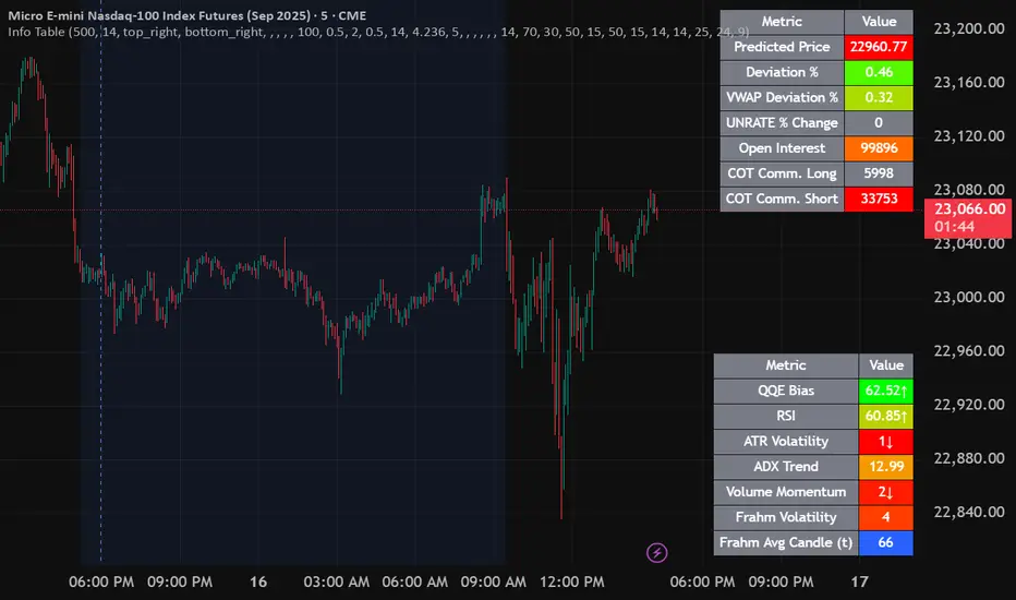
Info TableOverview
The Info Table V1 is a versatile TradingView indicator tailored for intraday futures traders, particularly those focusing on MESM2 (Micro E-mini S&P 500 futures) on 1-minute charts. It presents essential market insights through two customizable tables: the Main Table for predictive and macro metrics, and the New Metrics Table for momentum and volatility indicators. Designed for high-activity sessions like 9:30 AM–11:00 AM CDT, this tool helps traders assess price alignment, sentiment, and risk in real-time. Metrics update dynamically (except weekly COT data), with optional alerts for key conditions like volatility spikes or momentum shifts.
This indicator builds on foundational concepts like linear regression for predictions and adapts open-source elements for enhanced functionality. Gradient code is adapted from TradingView's Color Library. QQE logic is adapted from LuxAlgo's QQE Weighted Oscillator, licensed under CC BY-NC-SA 4.0. The script is released under the Mozilla Public License 2.0.
Key Features
Two Customizable Tables: Positioned independently (e.g., top-right for Main, bottom-right for New Metrics) with toggle options to show/hide for a clutter-free chart.
Gradient Coloring: User-defined high/low colors (default green/red) for quick visual interpretation of extremes, such as overbought/oversold or high volatility.
Arrows for Directional Bias: In the New Metrics Table, up (↑) or down (↓) arrows appear in value cells based on metric thresholds (top/bottom 25% of range), indicating bullish/high or bearish/low conditions.
Consensus Highlighting: The New Metrics Table's title cells ("Metric" and "Value") turn green if all arrows are ↑ (strong bullish consensus), red if all are ↓ (strong bearish consensus), or gray otherwise.
Predicted Price Plot: Optional line (default blue) overlaying the ML-predicted price for visual comparison with actual price action.
Alerts: Notifications for high/low Frahm Volatility (≥8 or ≤3) and QQE Bias crosses (bullish/bearish momentum shifts).
Main Table Metrics
This table focuses on predictive, positional, and macro insights:
ML-Predicted Price: A linear regression forecast using normalized price, volume, and RSI over a customizable lookback (default 500 bars). Gradient scales from low (red) to high (green) relative to the current price ± threshold (default 100 points).
Deviation %: Percentage difference between current price and predicted price. Gradient highlights extremes (±0.5% default threshold), signaling potential overextensions.
VWAP Deviation %: Percentage difference from Volume Weighted Average Price (VWAP). Gradient indicates if price is above (green) or below (red) fair value (±0.5% default).
FRED UNRATE % Change: Percentage change in U.S. unemployment rate (via FRED data). Cell turns red for increases (economic weakness), green for decreases (strength), gray if zero or disabled.
Open Interest: Total open MESM2 futures contracts. Gradient scales from low (red) to high (green) up to a hardcoded 300,000 threshold, reflecting market participation.
COT Commercial Long/Short: Weekly Commitment of Traders data for commercial positions. Long cell green if longs > shorts (bullish institutional sentiment); Short cell red if shorts > longs (bearish); gray otherwise.
New Metrics Table Metrics
This table emphasizes technical momentum and volatility, with arrows for quick bias assessment:
QQE Bias: Smoothed RSI vs. trailing stop (default length 14, factor 4.236, smooth 5). Green for bullish (RSI > stop, ↑ arrow), red for bearish (RSI < stop, ↓ arrow), gray for neutral.
RSI: Relative Strength Index (default period 14). Gradient from oversold (red, <30 + threshold offset, ↓ arrow if ≤40) to overbought (green, >70 - offset, ↑ arrow if ≥60).
ATR Volatility: Score (1–20) based on Average True Range (default period 14, lookback 50). High scores (green, ↑ if ≥15) signal swings; low (red, ↓ if ≤5) indicate calm.
ADX Trend: Average Directional Index (default period 14). Gradient from weak (red, ↓ if ≤0.25×25 threshold) to strong trends (green, ↑ if ≥0.75×25).
Volume Momentum: Score (1–20) comparing current to historical volume (lookback 50). High (green, ↑ if ≥15) suggests pressure; low (red, ↓ if ≤5) implies weakness.
Frahm Volatility: Score (1–20) from true range over a window (default 24 hours, multiplier 9). Dynamic gradient (green/red/yellow); ↑ if ≥7.5, ↓ if ≤2.5.
Frahm Avg Candle (Ticks): Average candle size in ticks over the window. Blue gradient (or dynamic green/red/yellow); ↑ if ≥0.75 percentile, ↓ if ≤0.25.
Arrows trigger on metric-specific logic (e.g., RSI ≥60 for ↑), providing directional cues without strict color ties.
Customization Options
Adapt the indicator to your strategy:
ML Inputs: Lookback (10–5000 bars) and RSI period (2+) for prediction sensitivity—shorter for volatility, longer for trends.
Timeframes: Individual per metric (e.g., 1H for QQE Bias to match higher frames; blank for chart timeframe).
Thresholds: Adjust gradients and arrows (e.g., Deviation 0.1–5%, ADX 0–100, RSI overbought/oversold).
QQE Settings: Length, factor, and smooth for fine-tuned momentum.
Data Toggles: Enable/disable FRED, Open Interest, COT for focus (e.g., disable macro for pure intraday).
Frahm Options: Window hours (1+), scale multiplier (1–10), dynamic colors for avg candle.
Plot/Table: Line color, positions, gradients, and visibility.
Ideal Use Case
Perfect for MESM2 scalpers and trend traders. Use the Main Table for entry confirmation via predicted deviations and institutional positioning. Leverage the New Metrics Table arrows for short-term signals—enter bullish on green consensus (all ↑), avoid chop on low volatility. Set alerts to catch shifts without constant monitoring.
Why It's Valuable
Info Table V1 consolidates diverse metrics into actionable visuals, answering critical questions: Is price mispriced? Is momentum aligning? Is volatility manageable? With real-time updates, consensus highlights, and extensive customization, it enhances precision in fast markets, reducing guesswork for confident trades.
Note: Optimized for futures; some metrics (OI, COT) unavailable on non-futures symbols. Test on demo accounts. No financial advice—use at your own risk.
The provided script reuses open-source elements from TradingView's Color Library and LuxAlgo's QQE Weighted Oscillator, as noted in the script comments and description. Credits are appropriately given in both the description and code comments, satisfying the requirement for attribution.
Regarding significant improvements and proportion:
The QQE logic comprises approximately 15 lines of code in a script exceeding 400 lines, representing a small proportion (<5%).
Adaptations include integration with multi-timeframe support via request.security, user-customizable inputs for length, factor, and smooth, and application within a broader table-based indicator for momentum bias display (with color gradients, arrows, and alerts). This extends the original QQE beyond standalone oscillator use, incorporating it as one of seven metrics in the New Metrics Table for confluence analysis (e.g., consensus highlighting when all metrics align). These are functional enhancements, not mere stylistic or variable changes.
The Color Library usage is via official import (import TradingView/Color/1 as Color), leveraging built-in gradient functions without copying code, and applied to enhance visual interpretation across multiple metrics.
The script complies with the rules: reused code is minimal, significantly improved through integration and expansion, and properly credited. It qualifies for open-source publication under the Mozilla Public License 2.0, as stated.
Normalized Open InterestNormalized Open Interest (nOI) — Indicator Overview
What it does
Normalized Open Interest (nOI) transforms raw futures open-interest data into a 0-to-100 oscillator, so you can see at a glance whether participation is unusually high or low—similar in spirit to an RSI but applied to open interest. The script positions today’s OI inside a rolling high–low range and paints it with contextual colours.
Core logic
Data source – Loads the built-in “_OI” symbol that TradingView provides for the current market.
Rolling range – Looks back a user-defined number of bars (default 500) to find the highest and lowest OI in that window.
Normalization – Calculates
nOI = (OI – lowest) / (highest – lowest) × 100
so 0 equals the minimum of the window and 100 equals the maximum.
Visual cues – Plots the oscillator plus fixed horizontal levels at 70 % and 30 % (or your own numbers). The line turns teal above the upper level, red below the lower, and neutral grey in between.
User inputs
Window Length (bars) – How many candles the indicator scans for the high–low range; larger numbers smooth the curve, smaller numbers make it more reactive.
Upper Threshold (%) – Default 70. Anything above this marks potentially crowded or overheated interest.
Lower Threshold (%) – Default 30. Anything below this marks low or capitulating interest.
Practical uses
Spot extremes – Values above the upper line can warn that the long side is crowded; values below the lower line suggest disinterest or short-side crowding.
Confirm breakouts – A price breakout backed by a sharp rise in nOI signals genuine engagement.
Look for divergences – If price makes a new high but nOI does not, participation might be fading.
Combine with volume or RSI – Layer nOI with other studies to filter false signals.
Tips
On intraday charts for non-crypto symbols the script automatically fetches daily OI data to avoid gaps.
Adjust the thresholds to 80/20 or 60/40 to fit your market and risk preferences.
Alerts, shading, or additional signal logic can be added easily because the oscillator is already normalised.

CGMALibrary "CGMA"
This library provides a function to calculate a moving average based on Chebyshev-Gauss Quadrature. This method samples price data more intensely from the beginning and end of the lookback window, giving it a unique character that responds quickly to recent changes while also having a long "memory" of the trend's start. Inspired by reading rohangautam.github.io
What is Chebyshev-Gauss Quadrature?
It's a numerical method to approximate the integral of a function f(x) that is weighted by 1/sqrt(1-x^2) over the interval . The approximation is a simple sum: ∫ f(x)/sqrt(1-x^2) dx ≈ (π/n) * Σ f(xᵢ) where xᵢ are special points called Chebyshev nodes.
How is this applied to a Moving Average?
A moving average can be seen as the "mean value" of the price over a lookback window. The mean value of a function with the Chebyshev weight is calculated as:
Mean = /
The math simplifies beautifully, resulting in the mean being the simple arithmetic average of the function evaluated at the Chebyshev nodes:
Mean = (1/n) * Σ f(xᵢ)
What's unique about this MA?
The Chebyshev nodes xᵢ are not evenly spaced. They are clustered towards the ends of the interval . We map this interval to our lookback period. This means the moving average samples prices more intensely from the beginning and the end of the lookback window, and less intensely from the middle. This gives it a unique character, responding quickly to recent changes while also having a long "memory" of the start of the trend.

Volatility Bias ModelVolatility Bias Model
Overview
Volatility Bias Model is a purely mathematical, non-indicator-based trading system that detects directional probability shifts during high volatility market phases. Rather than relying on classic tools like RSI or moving averages, this strategy uses raw price behavior and clustering logic to determine potential breakout direction based on recent market bias.
How It Works
Over a defined lookback window (default 10 bars), the strategy counts how many candles closed in the same direction (i.e., bullish or bearish).
Simultaneously, it calculates the price range during that window.
If volatility is above a minimum threshold and a clear directional bias is detected (e.g., >60% of closes are bullish), a trade is opened in the direction of that bias.
This approach assumes that when high volatility is coupled with directional closing consistency, the market is probabilistically more likely to continue in that direction.
ATR-based stop-loss and take-profit levels are applied, and trades auto-exit after 20 bars if targets are not hit.
Key Features
- 100% non-indicator-based logic
- Statistically-driven directional bias detection
- Works across all timeframes (1H, 4H, 1D)
- ATR-based risk management
- No pyramiding, slippage and commissions included
- Compatible with real-world backtesting conditions
Realism & Assumptions
To make this strategy more aligned with actual trading environments, it includes 0.05% commission per trade and a 1-point slippage on every entry and exit.
Additionally, position sizing is set at 10% of a $10,000 starting capital, and no pyramiding is allowed.
These assumptions help avoid unrealistic backtest results and make the performance metrics more representative of live conditions.
Parameter Explanation
Bias Window (10 bars): Number of past candles used to evaluate directional closings
Bias Threshold (0.60): Required ratio of same-direction candles to consider a bias valid
Minimum Range (1.5%): Ensures the market is volatile enough to avoid noise
ATR Length (14): Used to dynamically define stop-loss and target zones
Risk-Reward Ratio (2.0): Take-profit is set at twice the stop-loss distance
Max Holding Bars (20): Trades are closed automatically after 20 bars to prevent stagnation
Originality Note
Unlike common strategies based on oscillators or moving averages, this script is built on pure statistical inference. It models the market as a probabilistic process and identifies directional intent based on historical closing behavior, filtered by volatility. This makes it a non-linear, adaptive model grounded in real-world price structure — not traditional technical indicators.
Disclaimer
This strategy is for educational and experimental purposes only. It does not constitute financial advice. Always perform your own analysis and test thoroughly before applying with real capital.
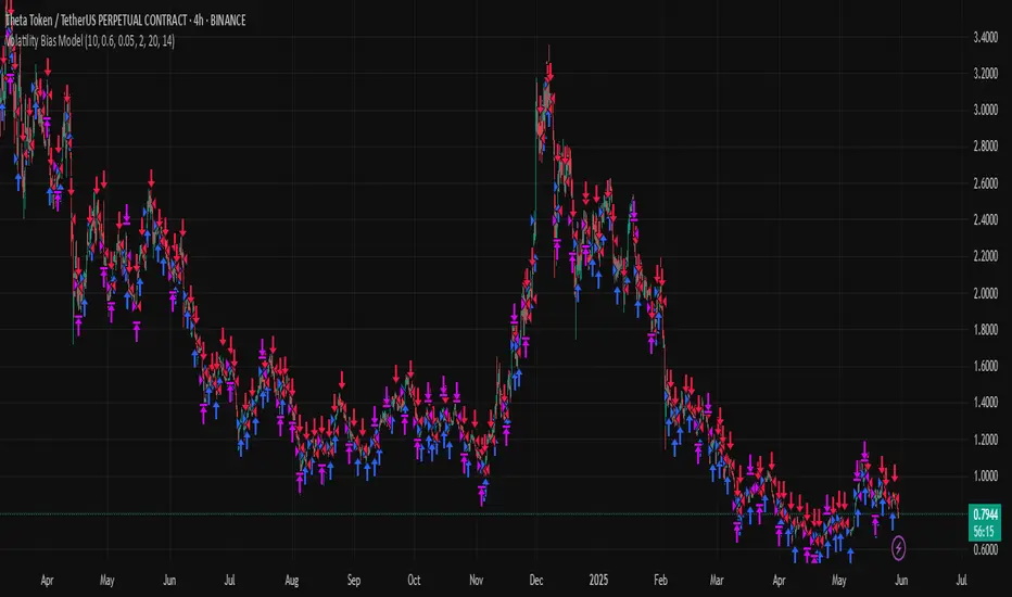
Real Time Swing Trap DetectorThe Real Time Swing Trap Detector is a minimalist, pro-grade tool for instantly spotting classic “bull traps” and “bear traps” on any chart.
This indicator identifies swing traps in real time by tracking significant swing highs and lows, then watching for fast, false breakouts (bull traps) and breakdowns (bear traps) within a user-defined window.
How it works:
Detects when price breaks a major swing high/low (using configurable lookback).
If price quickly reclaims the broken level within X bars (trap window), a trap is confirmed and a subtle icon (🐂 for bull, 🐻 for bear) is displayed on the chart—no labels, no clutter.
You can enable/disable alerts for bull/bear traps individually or together, and receive notifications the moment a trap is detected.
Use cases:
Spot and avoid classic market “fakeouts” that trap breakout traders.
Confirm SMC/ICT “Judas swing” setups, or filter for high-probability reversals.
Works on all timeframes and assets: stocks, crypto, forex, indices.
Inputs:
Swing Lookback Bars: How far back to define swing points (default: 50)
Major Swing Filter: Additional filter for only the most significant highs/lows (default: 200)
Trap Bars (Look Ahead): Window in which a trap must be confirmed (default: 10)
Enable Bull/Bear Trap Alerts: Toggle real-time alerts for each trap type.
Visuals:
🐻 icon below bar for bear trap (short squeeze/reversal)
🐂 icon above bar for bull trap (long squeeze/reversal)
How to set up alerts:
Add the indicator to your chart, open TradingView’s Alerts panel, and choose “Bear Trap Alert,” “Bull Trap Alert,” or “Any Trap Alert” for instant notifications.
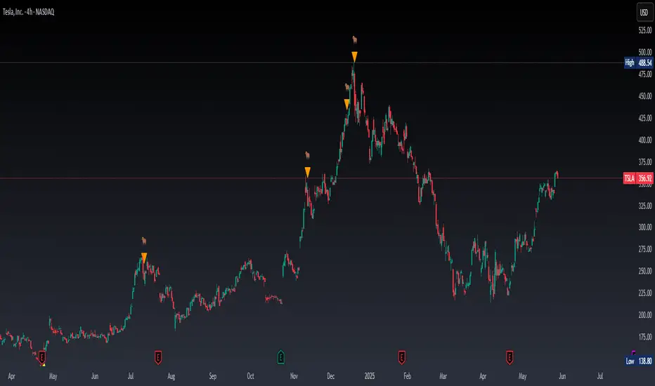
Market Manipulation Index (MMI)The Composite Manipulation Index (CMI) is a structural integrity tool that quantifies how chaotic or orderly current market conditions are, with the aim of detecting potentially manipulated or unstable environments. It blends two distinct mathematical models that assess price behavior in terms of both structural rhythm and predictability.
1. Sine-Fit Deviation Model:
This component assumes that ideal, low-manipulation price behavior resembles a smooth oscillation, such as a sine wave. It generates a synthetic sine wave using a user-defined period and compares it to actual price movement over an adaptive window. The error between the real price and this synthetic wave—normalized by price variance—forms the Sine-Based Manipulation Index. A high error indicates deviation from natural rhythm, suggesting structural disorder.
2. Predictability-Based Model:
The second component estimates how well current price can be predicted using recent price lags. A two-variable rolling linear regression is computed between the current price and two lagged inputs (close and close ). If the predicted price diverges from the actual price, this error—also normalized by price variance—reflects unpredictability. High prediction error implies a more manipulated or erratic environment.
3. Adaptive Mechanism:
Both components are calculated using an adaptive smoothing window based on the Average True Range (ATR). This allows the indicator to respond proportionally to market volatility. During high volatility, the analysis window expands to avoid over-sensitivity; during calm periods, it contracts for better responsiveness.
4. Composite Output:
The two normalized metrics are averaged to form the final CMI value, which is then optionally smoothed further. The output is scaled between 0 and 1:
0 indicates a highly structured, orderly market.
1 indicates complete structural breakdown or randomness.
Suggested Interpretation:
CMI < 0.3: Market is clean and structured. Trend-following or breakout strategies may perform better.
CMI > 0.7: Market is structurally unstable. Choppy price action, fakeouts, or manipulative behavior may dominate.
CMI 0.3–0.7: Transitional zone. Caution or reduced risk may be warranted.
This indicator is designed to serve as a contextual filter, helping traders assess whether current market conditions are conducive to structured strategies, or if discretion and defense are more appropriate.
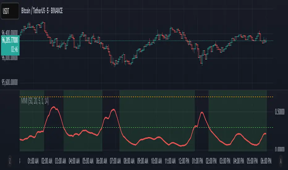
PumpC Opening Range Breakout (ORB) 5min Range📄 PumpC ORB 5-Minute Opening Range Breakout Indicator
✨ Overview
The PumpC ORB 5-Minute Opening Range Breakout indicator captures early session price action by tracking the high, low, and open of a defined 5-minute window at market open (customized for Futures or Stocks).
It plots breakout levels, extension targets, average range calculations, volume tracking, and provides visual and table-based data summaries.
This indicator is designed for traders seeking a complete, clean visualization of Opening Range Breakouts (ORB) with flexible customization.
⚙️ Main Features
Opening Range Box (ORB Box) Draws a box around the high and low of the first 5-minute session (8:30–8:35 ET for Futures, 9:30–9:35 ET for Stocks). Box extends from the session open to the session close (4:00 PM ET). Option to enable/disable historical boxes. Box color and opacity are customizable. Core ORB Levels Open Level: Plots the open price of the 5-minute ORB window. ORB Levels: Plots breakout levels at multiples: +0.5x the range +1.5x the range (customizable factor) Each level has independent color settings and visibility toggles. Option to show or hide historic extension levels. Table Display Compact table in the top-right corner showing: ORB ATR (average range) ORB ATR in ticks Today's ORB range ORB Volume ATR (average volume during ORB) Today's ORB Volume Volume is formatted automatically into "K" (thousands) or "M" (millions) for readability. Background Highlights After the ORB window closes: Blue highlight if today's ORB range is greater than the 10-day ATR average. Orange highlight if today's ORB range is smaller than the 10-day ATR average. Helps quickly assess relative strength or weakness compared to historical behavior. Alerts Breakout Confirmations: Fires when price closes above ORB High or below ORB Low. Fallout Traps: Alerts when price wick crosses ORB High/Low but closes back inside the range. Alerts use clean titles and simple messages for easy identification.
🔧 Inputs and Customization
Mode Toggle: Choose between Futures (8:30 ET open) or Stocks (9:30 ET open). Show/Hide Labels: Control label visibility for ORB and extension levels. Line Width Control: Customize thickness for ORB lines and extension levels. ORB Level Level Visibility: Independently enable or disable each extension line. Table Appearance: Customize table background color, font color, and padding. ORB Box Settings: Customize box color and control whether historical boxes are drawn.
📚 How to Use
Select Mode: Choose Futures or Stocks depending on your instrument. Observe the Opening Range: Focus on the ORB High and ORB Low during the first 5 minutes after the open. Monitor Breakouts: Breakout alerts will fire when price closes outside the ORB range, signaling potential continuation. Watch for Fallout Traps: Fallout alerts signal when price briefly wicks above/below but closes back inside the ORB range. Use Table Metrics: Instantly compare today's ORB range and volume versus historical averages to assess session strength or weakness.
🛡️ Notes
Best used on the 1-minute or 5-minute chart for intraday trading. Ensure your TradingView chart time zone is set to New York for correct functioning. Alerts must be manually configured after adding the indicator to your chart.
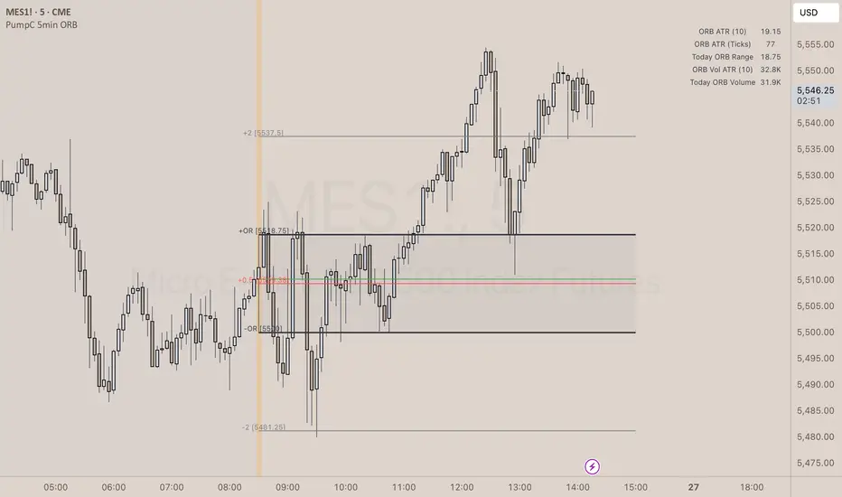
Uptrick: Dynamic Z-Score DeviationOverview
Uptrick: Dynamic Z‑Score Deviation is a trading indicator built in Pine Script that combines statistical filters and adaptive smoothing to highlight potential reversal points in price action. It combines a hybrid moving average, dual Z‑Score analysis on both price and RSI, and visual enhancements like slope‑based coloring, ATR‑based shadow bands, and dynamically scaled reversal signals.
Introduction
Statistical indicators like Z‑Scores measure how far a value deviates from its average relative to the typical variation (standard deviation). Standard deviation quantifies how dispersed a set of values is around its mean. A Z‑Score of +2 indicates a value two standard deviations above the mean, while -2 is two below. Traders use Z‑Scores to spot unusually high or low readings that may signal overbought or oversold conditions.
Moving averages smooth out price data to reveal trends. The Arnaud Legoux Moving Average (ALMA) reduces lag and noise through weighted averaging. A Zero‑Lag EMA (approximated here using a time‑shifted EMA) seeks to further minimize delay in following price. The RSI (Relative Strength Index) is a momentum oscillator that measures recent gains against losses over a set period.
ATR (Average True Range) gauges market volatility by averaging the range between high and low over a lookback period. Shadow bands built using ATR give a visual mood of volatility around a central trend line. Together, these tools inform a dynamic but statistically grounded view of market extremes.
Purpose
The main goal of this indicator is to help traders spot short‑term reversal opportunities on lower timeframes. By requiring both price and momentum (RSI) to exhibit statistically significant deviations from their norms, it filters out weak setups and focuses on higher‑probability mean‑reversion zones. Reversal signals appear when price deviates far enough from its hybrid moving average and RSI deviates similarly in the same direction. This makes it suitable for discretionary traders seeking clean entry cues in volatile environments.
Originality and Uniqueness
Uptrick: Dynamic Z‑Score Deviation distinguishes itself from standard reversal or mean‑reversion tools by combining several elements into a single framework:
A composite moving average (ALMA + Zero‑Lag EMA) for a smooth yet responsive baseline
Dual Z‑Score filters on price and RSI rather than relying on a single measure
Adaptive visual elements, including slope‑aware coloring, multi‑layer ATR shadows, and signal sizing based on combined Z‑Score magnitude
Most indicators focus on one aspect—price envelopes or RSI thresholds—whereas Uptrick: Dynamic Z‑Score Deviation requires both layers to align before signaling. Its visual design aids quick interpretation without overwhelming the chart.
Why these indicators were merged
Every component in Uptrick: Dynamic Z‑Score Deviation has a purpose:
• ALMA: provides a smooth moving average with reduced lag and fewer false crossovers than a simple SMA or EMA.
• Zero‑Lag EMA (ZLMA approximation): further reduces the delay relative to price by applying a time shift to EMA inputs. This keeps the composite MA closer to current price action.
• RSI and its EMA filter: RSI measures momentum. Applying an EMA filter on RSI smooths out false spikes and confirms genuine overbought or oversold momentum.
• Dual Z‑Scores: computing Z‑Scores on both the distance between price and the composite MA, and on smoothed RSI, ensures that signals only fire when both price and momentum are unusually stretched.
• ATR bands: using ATR‑based shadow layers visualizes volatility around the MA, guiding traders on potential support and resistance zones.
At the end, these pieces merge into a single indicator that detects statistically significant mean reversions while staying adaptive to real‑time volatility and momentum.
Calculations
1. Compute ALMA over the chosen MA length, offset, and sigma.
2. Approximate ZLMA by applying EMA to twice the price minus the price shifted by the MA length.
3. Calculate the composite moving average as the average of ALMA and ZLMA.
4. Compute raw RSI and smooth it with ALMA. Apply an EMA filter to raw RSI to reduce noise.
5. For both price and smoothed RSI, calculate the mean and standard deviation over the Z‑Score lookback period.
6. Compute Z‑Scores:
• z_price = (current price − composite MA mean) / standard deviation of price deviations
• z_rsi = (smoothed RSI − mean RSI) / standard deviation of RSI
7. Determine reversal conditions: both Z‑Scores exceed their thresholds in the same direction, RSI EMA is in oversold/overbought zones (below 40 or above 60), and price movement confirms directionality.
8. Compute signal strength as the sum of the absolute Z‑Scores, then classify into weak, medium, or strong.
9. Calculate ATR over the chosen period and multiply by layer multipliers to form shadow widths.
10.Derive slope over the chosen slope length and color the MA line and bars based on direction, optionally smoothing color transitions via EMA on RGB channels.
How this indicator actually works
1. The script begins by smoothing price data with ALMA and approximating a zero‑lag EMA, then averaging them for the main MA.
2. RSI is calculated, then smoothed and filtered.
3. Using a rolling window, the script computes statistical measures for both price deviations and RSI.
4. Z‑Scores tell how far current values lie from their recent norms.
5. When both Z‑Scores cross configured thresholds and momentum conditions align, reversal signals are flagged.
6. Signals are drawn with size and color reflecting strength.
7. The MA is plotted with dynamic coloring; ATR shadows are layered beneath to show volatility envelopes.
8. Bars can be colored to match MA slope, reinforcing trend context.
9. Alert conditions allow automated notifications when signals occur.
Inputs
Main Length: Main MA Length. Sets the period for ALMA and ZLMA.
RSI Length: RSI Length. Determines the lookback for momentum calculations.
Z-Score Lookback: Z‑Score Lookback. Window for mean and standard deviation computations.
Price Z-Score Threshold: Price Z‑Score Threshold. Minimum deviation required for price.
RSI Z-Score threshold: RSI Z‑Score Threshold. Minimum deviation required for momentum.
RSI EMA Filter Length: RSI EMA Filter Length. Smooths raw RSI readings.
ALMA Offset: Controls ALMA’s focal point in the window.
ALMA Sigma: Adjusts ALMA’s smoothing strength.
Show Reversal Signals : Toggle to display reversal signal markers.
Slope Sensitivity: Length for slope calculation. Higher values smooth slope changes.
Use Bar Coloring: Enables coloring of price bars based on MA slope.
Show MA Shadow: Toggle for ATR‑based shadow bands.
Shadow Layer Count: Number of shadow layers (1–4).
Base Shadow ATR Multiplier: Multiplier for ATR when sizing the first band.
Smooth Color Transitions (boolean): Smooths RGB transitions for line and shadows, if enabled.
ATR Length for Shadow: ATR Period for computing volatility bands.
Use Dynamic Signal Size: Toggles dynamic scaling of reversal symbols.
Features
Moving average smoothing: a hybrid of ALMA and Zero‑Lag EMA that balances responsiveness and noise reduction.
Slope coloring: MA line and optionally price bars change color based on trend direction; color transitions can be smoothed for visual continuity.
ATR shadow layers: translucent bands around the MA show volatility envelopes; up to four concentric layers help gauge distance from normal price swings.
Dual Z‑Score filters: price and momentum must both deviate beyond thresholds to trigger signals, reducing false positives.
Dynamic signal sizing: reversal markers scale in size based on the combined Z‑Score magnitude, making stronger signals more prominent.
Adaptive visuals: optional smoothing of color channels creates gradient effects on lines and fills for a polished look.
Alert conditions: built‑in buy and sell alerts notify traders when reversal setups emerge.
Conclusion
Uptrick: Dynamic Z‑Score Deviation delivers a structured way to identify short‑term reversal opportunities by fusing statistical rigor with adaptive smoothing and clear visual cues. It guides traders through multiple confirmation layers—hybrid moving average, dual Z‑Score analysis, momentum filtering, and volatility envelopes—while keeping the chart clean and informative.
Disclaimer
This indicator is provided for informational and educational purposes only and does not constitute financial advice. Trading carries risk and may not be suitable for all participants. Past performance is not indicative of future results. Always do your own analysis and risk management before making trading decisions.
RSI SiaThis script is a custom indicator for TradingView written in Pine Script version 5. It calculates the Relative Strength Index (RSI) and uses it to generate trading signals. Here's a breakdown of what the script does:
Key Features:
RSI Calculation:
The script calculates the RSI using a 14-period window.
It also calculates the momentum of the RSI over a 9-period window (rsi delta) and a simple moving average (SMA) of the RSI over a 3-period window (rsi sma).
Composite Index (CI):
The composite index is calculated as the sum of rsi delta and rsi sma.
Horizontal Lines and Zones:
Several horizontal lines are plotted at different levels (e.g., 20, 40, 60, 80, 120, 150, 180) to indicate overbought and oversold conditions.
Filled zones are created between certain levels to highlight areas of interest.
Moving Averages:
The script plots SMA and EMA of the RSI when Enable RSI ma is set to true.
It also plots moving averages of the composite index.
Crossover Signals:
The script detects bullish and bearish crossovers between the SMA and EMA of the RSI.
It plots shapes (labels) on the chart to indicate buy (BUY) and sell (SELL) signals based on these crossovers.
Usage:
Enable RSIma: This input allows you to enable or disable the plotting of RSI moving averages.
i1: This variable is used to adjust the vertical position of the composite index and its moving averages.
Visualization:
The RSI is plotted in black.
The RSI fast trigger line (SMA of RSI) is plotted in green when enabled.
The RSI slow trigger line (EMA of RSI) is plotted in orange when enabled.
The composite index and its moving averages are plotted in red, green, and orange.
Buy and sell signals are indicated with green and red labels, respectively.
This script can be used to identify potential trading opportunities based on RSI crossovers and the composite index.
volume profile ranking indicator📌 Introduction
This script implements a volume profile ranking indicato for TradingView. It is designed to visualize the distribution of traded volume over price levels within a defined historical window. Unlike TradingView’s built-in Volume Profile, this script gives full customization of the profile drawing logic, binning, color gradient, and the ability to anchor the profile to a specific date.
⚙️ How It Works (Logic)
1. Inputs
➤POC Lookback Days (lookback): Defines how many bars (days) to look back from a selected point to calculate the volume distribution.
➤Bin Count (bin_count): Determines how many price bins (horizontal levels) the price range will be divided into.
➤Use Custom Lookback Date (useCustomDate): Enables/disables manually selecting a backtest start date.
➤Custom Lookback Date (customDate): When enabled, the profile will calculate volume based on this date instead of the most recent bar.
2. Target Bar Determination
➤If a custom date is selected, the script searches for the bar closest to that date within 1000 bars.
➤If not, it defaults to the latest bar (bar_index).
➤The profile is drawn only when the current bar is close to the target bar (within ±2 bars), to avoid unnecessary recalculations and performance issues.
3. Volume Binning
➤The price range over the lookback window is divided into bin_count segments.
➤For each bar within the lookback window, its volume is added to the appropriate bin based on price.
➤If the price falls outside the expected range, it is clamped to the first or last bin.
4. Ranking and Sorting
➤A bubble sort ranks each bin by total volume.
➤The most active bin (POC, or Point of Control) is highlighted with a thicker bar.
5. Rendering
➤Horizontal bars (line.new) represent volume intensity in each price bin.
➤Each bar is color-coded by volume heat: more volume = more intense color.
➤Labels (label.new) show:
➤Total volume
➤Rank
➤Percentage of total volume
➤Price range of the bin
🧑💻 How to Use
1. Add the Script to Your Chart
➤Copy the code into TradingView’s Pine Script editor and add it to your chart.
2. Set Lookback Period
➤Default is 252 bars (about one year for daily charts), but can be changed via the input.
3. (Optional) Use Custom Date
●Toggle "Use Custom Lookback Date" to true.
➤Pick a date in the "Custom Lookback Date" input to anchor the profile.
4. Analyze the Volume Distribution
➤The longest (thickest) red/orange bar represents the Point of Control (POC) — the price with the most volume traded.
➤Other bars show volume distribution across price.
➤Labels display useful metrics to evaluate areas of high/low interest.
✅ Features
🔶 Customizable anchor point (custom date).
🔶Adjustable bin count and lookback length.
🔶 Clear visualization with heatmap coloring.
🔶 Lightweight and performance-optimized (especially with the shouldDrawProfile filter)

SnowdexUtilsLibrary "SnowdexUtils"
the various function that often use when create a strategy trading.
f_backtesting_date(train_start_date, train_end_date, test_date, deploy_date)
Backtesting within a specific window based on deployment and testing dates.
Parameters:
train_start_date (int) : the start date for training the strategy.
train_end_date (int) : the end date for training the strategy.
test_date (bool) : if true, backtests within the period from `train_end_date` to the current time.
deploy_date (bool) : if true, the strategy backtests up to the current time.
Returns: given time falls within the specified window for backtesting.
f_init_ma(ma_type, source, length)
Initializes a moving average based on the specified type.
Parameters:
ma_type (simple string) : the type of moving average (e.g., "RMA", "EMA", "SMA", "WMA").
source (float) : the input series for the moving average calculation.
length (simple int) : the length of the moving average window.
Returns: the calculated moving average value.
f_init_tp(side, entry_price, rr, sl_open_position)
Calculates the target profit based on entry price, risk-reward ratio, and stop loss. The formula is `tp = entry price + (rr * (entry price - stop loss))`.
Parameters:
side (bool) : the trading side (true for long, false for short).
entry_price (float) : the entry price of the position.
rr (float) : the risk-reward ratio.
sl_open_position (float) : the stop loss price for the open position.
Returns: the calculated target profit value.
f_round_up(number, decimals)
Rounds up a number to a specified number of decimals.
Parameters:
number (float)
decimals (int)
Returns: The rounded-up number.
f_get_pip_size()
Calculates the pip size for the current instrument.
Returns: Pip size adjusted for Forex instruments or 1 for others.
f_table_get_position(value)
Maps a string to a table position constant.
Parameters:
value (string) : String representing the desired position (e.g., "Top Right").
Returns: The corresponding position constant or `na` for invalid values.
