Average Candle RangeThis indicator calculates and displays the average trading range of candles over a specified period, helping traders identify volatility patterns and potential trading opportunities.
Features:
- Customizable lookback period (1-500 bars)
- Clean visual display in a top-right table overlay
- High-precision calculation showing 10 decimal places
- Real-time updates with each new bar
How it Works:
The indicator calculates the range of each candle (High - Low) and then computes the Simple Moving Average (SMA) of these ranges over your specified lookback period. The result is displayed in an easy-to-read table overlay.
Use Cases:
- Volatility Analysis: Monitor market volatility trends
- Position Sizing: Help determine position sizes based on average price movements
- Trading Strategy Development: Use as a reference for setting stop losses and take profits
- Market Phase Identification: Help identify high vs low volatility market phases
Settings:
- Lookback Period: Default is 140 bars, adjustable from 1 to 500
Note:
The indicator displays values with 10 decimal places for high-precision analysis, particularly useful in markets with small price movements.
Cari dalam skrip untuk "新泻天鹅vs川崎前锋"

Exponential Avg Body Size Green vs RedDescription :
This indicator calculates and plots the Exponential Moving Average (EMA) of green and red candlestick body sizes, allowing traders to easily visualize market momentum and sentiment shifts. The script includes the following features:
Customizable EMA Period: Users can set the number of candles to calculate the EMA through an input setting, with a default value of 21.
Separate Green and Red Candle Averages: Differentiates between bullish (green) and bearish (red) candlestick movements, plotting them as distinct lines.
Dynamic Range Control: Users can adjust the chart range (e.g., -50 to 50) for better visibility of the plotted lines.
Baseline for Reference: A horizontal baseline at 0 serves as a visual aid for easier interpretation.
Standalone Indicator Pane: The script is designed to display in a separate pane, preventing overlap with the price chart.
Use Case:
This indicator is ideal for traders seeking to analyze the relative strength of bullish versus bearish price movements over a specific period. The separation of green and red averages helps identify trends, potential reversals, or shifts in momentum.

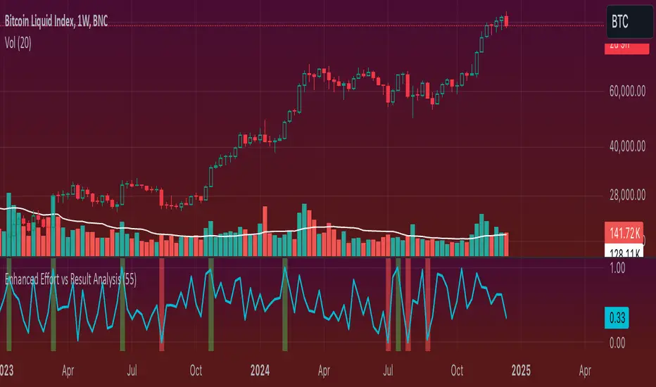
Enhanced Effort vs Result Analysis V.2How to Use in Trading
A. Confirm Breakouts
Check if the Effort-Result Ratio or Z-Score spikes above the Upper Band or Z > +2:
Suggests a strong, efficient price move.
Supports breakout continuation.
B. Identify Reversal or Exhaustion
Look for Effort-Result Ratio or Z-Score dropping below the Lower Band or Z < -2:
Indicates high effort but low price movement (inefficiency).
Often signals potential trend reversal or consolidation.
C. Assess Efficiency of Trends
Use Relative Efficiency Index (REI):
REI near 1 during a trend → Confirms strength (efficient movement).
REI near 0 → Weak or inefficient movement, likely signaling exhaustion.
D. Evaluate Volume-Price Relationship
Monitor the Volume-Price Correlation:
Positive correlation (+1): Confirms price is driven by volume.
Negative correlation (-1): Indicates divergence; price moves independently of volume (potential warning signal).
3. Example Scenarios
Scenario 1: Breakout Confirmation
Effort-Result Ratio spikes above the Upper Band.
Z-Score exceeds +2.
REI approaches 1.
Volume-Price Correlation is positive (near +1).
Action: Strong breakout confirmation → Trend continuation likely.
Scenario 2: Reversal or Exhaustion
Effort-Result Ratio drops below the Lower Band.
Z-Score is below -2.
REI approaches 0.
Volume-Price Correlation weakens or turns negative.
Action: Signals trend exhaustion → Watch for reversal or consolidation.
Scenario 3: Range-Bound Market
Effort-Result Ratio stays within the Bollinger Bands.
Z-Score remains between -1 and +1.
REI fluctuates around 0.5 (neutral efficiency).
Volume-Price Correlation hovers near 0.
Action: Normal conditions → Look for breakout signals before acting.
*IMPORTANT*
There is a problem with the overlay ... How to fix some of it
The Standard Deviation bands dont work while the other variable activated so Id suggest deselecting them. The fix for this is to make sure you have the background selected and by doing this it will highlight on the chart ( you may need to increase the opacity ) when the bands ( Second standard deviation) are touched.
- Also you can use them all at once if you can but you do not need to
G&S SMT### Description of the Pine Script
This Pine Script is designed to identify **Smart Money Technique (SMT)** setups between **Gold (GC1!)** and **Silver (SI1!) Futures** on a **15-minute timeframe**. It specifically looks for divergences between the price movements of Gold and Silver over the last 4 candles and compares it with the next candle's price movement. The script provides **Bullish** and **Bearish** signals for SMT during a specified time range of **8:45 AM EST to 10:30 AM EST**.
### Key Features of the Script:
1. **Futures Symbols**:
- The script uses **Gold Futures (GC1!)** and **Silver Futures (SI1!)** on a 15-minute timeframe to monitor their price movements.
2. **Time Range Filtering**:
- The signals are only active between **8:45 AM EST and 10:30 AM EST**, ensuring that the script only signals within the most relevant trading hours for your strategy.
3. **SMT Calculation (Last 4 Candles vs Next Candle)**:
- **Gold and Silver Price Change Calculation**: The script compares the price changes of **Gold** and **Silver** over the **last 4 candles** and then compares them with the price movement of the **next candle**:
- **Bullish SMT**: Occurs when Gold shows an increase in the last 4 candles while Silver shows a decrease, and both Gold and Silver show an increase in the next candle.
- **Bearish SMT**: Occurs when Gold shows a decrease in the last 4 candles while Silver shows an increase, and both Gold and Silver show a decrease in the next candle.
4. **Bullish and Bearish Signals**:
- **Bullish SMT Signal**: The script will plot a **green** arrow below the bar when a Bullish SMT setup is identified.
- **Bearish SMT Signal**: A **red** arrow above the bar is plotted when a Bearish SMT setup is identified.
5. **Gold and Silver Difference Plot**:
- The difference between the prices of **Gold** and **Silver** is plotted as a **blue line**, giving a visual representation of the relationship between the two assets. When the difference line moves significantly, it can indicate a potential divergence or convergence in the prices of Gold and Silver.
### Script Logic Breakdown:
1. **Price Change for Last 4 Candles**:
- The script calculates the price change for Gold and Silver from the 4th-to-last candle to the last candle.
- `gold_change_last4` and `silver_change_last4` calculate these price differences.
2. **Price Change for Next Candle**:
- It then calculates the price change from the last candle to the next candle.
- `gold_change_next` and `silver_change_next` calculate these price differences.
3. **Bullish SMT Condition**:
- If Gold increased while Silver decreased in the last 4 candles, and both Gold and Silver show an increase in the next candle, it indicates a **Bullish SMT**.
4. **Bearish SMT Condition**:
- If Gold decreased while Silver increased in the last 4 candles, and both Gold and Silver show a decrease in the next candle, it indicates a **Bearish SMT**.
5. **Time Filter**:
- Signals are only plotted when the current time is between **8:45 AM EST and 10:30 AM EST** to match your preferred trading hours.
### Visualization:
- **Bullish Signals**: Plotted as **green arrows** below the bars when a Bullish SMT setup is identified.
- **Bearish Signals**: Plotted as **red arrows** above the bars when a Bearish SMT setup is identified.
- **Gold - Silver Difference**: A **blue line** is plotted to show the price difference between Gold and Silver, helping visualize any divergence.
### How It Helps:
- **Divergence Identification**: This script highlights potential divergences between Gold and Silver Futures, which can provide insights into market sentiment and smart money movements.
- **Focus on Relevant Time Frame**: By filtering signals between 8:45 AM EST and 10:30 AM EST, you are focusing on a timeframe that can be more beneficial for trading.
- **Visual Clarity**: The arrows and the price difference line provide clear signals and a visual representation of the relationship between Gold and Silver, helping you make informed trading decisions.
This script is an automated approach to detecting **SMT setups** and helping traders recognize when Gold and Silver might be signaling a bullish or bearish move based on their divergence patterns.

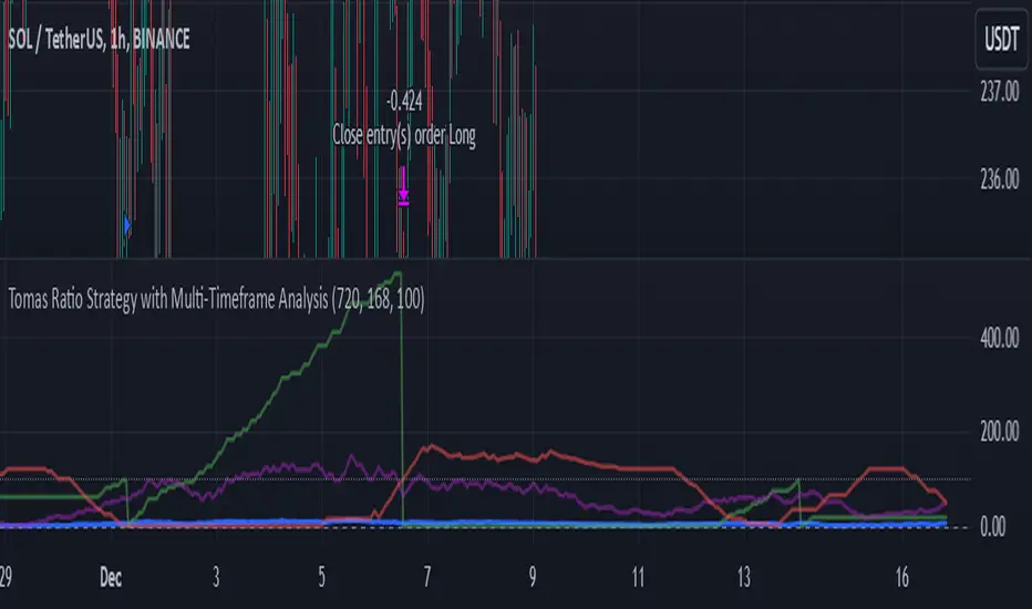
Tomas Ratio Strategy with Multi-Timeframe AnalysisHello,
I would like to present my new indicator I have compiled together inspired by Calmar Ratio which is a ratio that measures gains vs losers but with a little twist.
Basically the idea is that if HLC3 is above HLC3 (or previous one) it will count as a gain and it will calculate the percentage of winners in last 720 hourly bars and then apply 168 hour standard deviation to the weekly average daily gains.
The idea is that you're supposed to buy if the thick blue line goes up and not buy if it goes down (signalized by the signal line). I liked that idea a lot, but I wanted to add an option to fire open and close signals. I have also added a logic that it not open more trades in relation the purple line which shows confidence in buying.
As input I recommend only adjusting the amount of points required to fire a signal. Note that the lower amount you put, the more open trades it will allow (and vice versa)
Feel free to remove that limiter if you want to. It works without it as well, this script is meant for inexperienced eye.
I will also publish a indicator script with this limiter removed and alerts added for you to test this strategy if you so choose to.
Also, I have added that the trades will enter only if price is above 720 period EMA
Disclaimer
This strategy is for educational purposes only and should not be considered financial advice. Always backtest thoroughly and adjust parameters based on your trading style and market conditions.
Made in collaboration with ChatGPT.
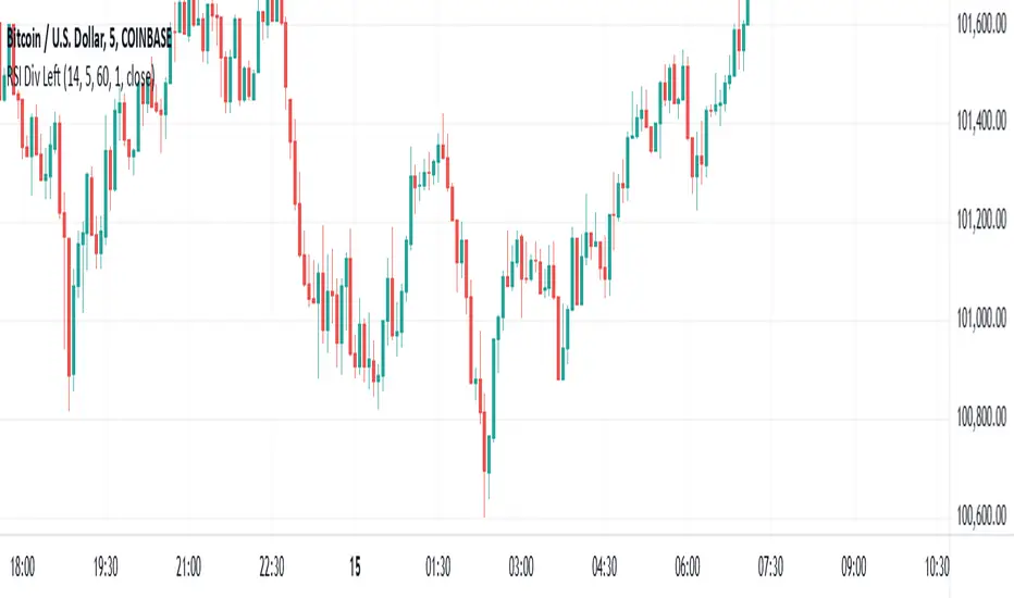
RSI Divergence - Left Candles Onlyrsi
The **RSI Divergence** indicator in this script is designed to highlight **divergence** between the **Relative Strength Index (RSI)** and **price action** on a chart. Divergence can be a key signal for potential trend reversals or continuation in technical analysis.
### **Key Components of the Indicator:**
1. **RSI Calculation:**
- The **Relative Strength Index (RSI)** is calculated using a typical 14-period length, but the user can customize this input.
- RSI is a momentum oscillator that measures the speed and change of price movements, oscillating between 0 and 100. Values above 70 indicate overbought conditions, and values below 30 indicate oversold conditions.
2. **Divergence Logic:**
- **Bullish Divergence:** Occurs when the price forms a **lower low**, but the RSI forms a **higher low**. This suggests that despite price continuing to drop, momentum (RSI) is strengthening, which may indicate a potential price reversal to the upside.
- **Bearish Divergence:** Occurs when the price forms a **higher high**, but the RSI forms a **lower high**. This indicates that even though price is rising, the momentum (RSI) is weakening, which could signal a price reversal to the downside.
3. **Pivot Identification:**
- The script identifies **pivot points** (local highs and lows) on both price and RSI.
- **Bullish Divergence:** A lower price low with a higher RSI low.
- **Bearish Divergence:** A higher price high with a lower RSI high.
4. **Lookback Periods:**
- **Lookback Left (lookbackLeft):** Defines the number of bars to look back for pivot confirmation. This allows for adjusting the sensitivity of the divergence.
- The **divergence range** is constrained by two parameters:
- **Minimum range (rangeLower):** The minimum number of bars for divergence to be considered.
- **Maximum range (rangeUpper):** The maximum number of bars for divergence to be considered.
5. **Signal Generation and Plotting:**
- When a **bullish divergence** is detected, a **green label** is plotted below the bar where the divergence occurs.
- When a **bearish divergence** is detected, a **red label** is plotted above the bar.
- The script uses **`plotshape()`** to plot these labels on the chart.
6. **Alerts:**
- Alerts are configured for both **bullish** and **bearish divergences** so that you can be notified when a divergence signal occurs.
---
### **How the Indicator Works:**
- The RSI and price action are compared using **pivots**: The script checks whether the price and RSI are forming new highs or lows within the specified **lookback period**.
- If the conditions for divergence (higher/lower RSI pivot vs price pivot) are met, a signal is plotted on the chart.
- The script helps to visually identify potential reversal points and allows users to set alerts for these divergence signals.
---
### **Use Case:**
- This script is useful for traders looking to trade potential trend reversals based on **divergence** between price and RSI.
- **Bullish divergence** can indicate a **buy** opportunity, while **bearish divergence** can suggest a **sell** opportunity.
- The indicator works best in **volatile markets** and when combined with other technical analysis tools for confirmatio
Weis Wave Max█ Overview
Weis Wave Max is the result of my weis wave study.
David Weis said,
"Trading with the Weis Wave involves changes in behavior associated with springs, upthrusts, tests of breakouts/breakdowns, and effort vs reward. The most common setup is the low-volume pullback after a bullish/bearish change in behavior."
THE STOCK MARKET UPDATE (February 24, 2013)
I inspired from his sentences and made this script.
Its Main feature is to identify the largest wave in Weis wave and advantageous trading opportunities.
█ Features
This indicator includes several features related to the Weis Wave Method.
They help you analyze which is more bullish or bearish.
Highlight Max Wave Value (single direction)
Highlight Abnormal Max Wave Value (both directions)
Support and Resistance zone
Signals and Setups
█ Usage
Weis wave indicator displays cumulative volume for each wave.
Wave volume is effective when analyzing volume from VSA (Volume Spread Analysis) perspective.
The basic idea of Weis wave is large wave volume hint trend direction. This helps identify proper entry point.
This indicator highlights max wave volume and displays the signal and then proper Risk Reward Ratio entry frame.
I defined Change in Behavior as max wave volume (single direction).
Pullback is next wave that does not exceed the starting point of CiB wave (LH sell entry, HL buy entry).
Change in Behavior Signal ○ appears when pullback is determined.
Change in Behavior Setup (Entry frame) appears when condition of Min/Max Pullback is met and follow through wave breaks end point of CiB wave.
This indicator has many other features and they can also help a user identify potential levels of trade entry and which is more bullish or bearish.
In the screenshot below we can see wave volume zones as support and resistance levels. SOT and large wave volume /delta price (yellow colored wave text frame) hint stopping action.
█ Settings
Explains the main settings.
-- General --
Wave size : Allows the User to select wave size from ① Fixed or ② ATR. ② ATR is Factor x ATR(Length).
Display : Allows the User to select how many wave text and zigzag appear.
-- Wave Type --
Wave type : Allows the User to select from Volume or Volume and Time.
Wave Volume / delta price : Displays Wave Volume / delta price.
Simplified value : Allows the User to select wave text display style from ① Divisor or ② Normalized. Normalized use SMA.
Decimal : Allows the User to select the decimal point in the Wave text.
-- Highlight Abnormal Wave --
Highlight Max Wave value (single direction) : Adds marks to the Wave text to highlight the max wave value.
Lookback : Allows the User to select how many waves search for the max wave value.
Highlight Abnormal Wave value (both directions) : Changes wave text size, color or frame color to highlight the abnormal wave value.
Lookback : Allows the User to select SMA length to decide average wave value.
Large/Small factor : Allows the User to select the threshold large wave value and small wave value. Average wave value is 1.
delta price : Highlights large delta price by large wave text size, small by small text size.
Wave Volume : Highlights large wave volume by yellow colored wave text, small by gray colored.
Wave Volume / delta price : highlights large Wave Volume / delta price by yellow colored wave text frame, small by gray colored.
-- Support and Resistance --
Single side Max Wave Volume / delta price : Draws dashed border box from end point of Max wave volume / delta price level.
Single side Max Wave Volume : Draws solid border box from start point of Max wave volume level.
Bias Wave Volume : Draws solid border box from start point of bias wave volume level.
-- Signals --
Bias (Wave Volume / delta price) : Displays Bias mark when large difference in wave volume / delta price before and after.
Ratio : Decides the threshold of become large difference.
3Decrease : Displays 3D mark when a continuous decrease in wave volume.
Shortening Of the Thrust : Displays SOT mark when a continuous decrease in delta price.
Change in Behavior and Pullback : Displays CiB mark when single side max wave volume and pullback.
-- Setups --
Change in Behavior and Pullback and Breakout : Displays entry frame when change in behavior and pullback and then breakout.
Min / Max Pullback : Decides the threshold of min / max pullback.
If you need more information, please read the indicator's tooltip.
█ Conclusion
Weis Wave is powerful interpretation of volume and its tell us potential trend change and entry point which can't find without weis wave.
It's not the holy grail, but improve your chart reading skills and help you trade rationally (at least from VSA perspective).

ADX and DI Trend meter and status table IndicatorThis ADX (Average Directional Index) and DI (Directional Indicator) indicator helps identify:
Trend Direction & Strength:
LONG: +DI above -DI with ADX > 20
SHORT: -DI above +DI with ADX > 20
RANGE: ADX < 20 indicates choppy/sideways market
Trading Signals:
Bullish: +DI crosses above -DI (green triangle)
Bearish: -DI crosses below +DI (red triangle)
ADX Strength Levels:
Strong: ADX ≥ 50
Moderate: ADX 30-49
Weak: ADX 20-29
No Trend: ADX < 20
Best Uses:
Trend confirmation before entering trades
Identifying ranging vs trending markets
Exit signal when trend weakens
Works well on multiple timeframes
Most effective in combination with other indicators
The table displays current trend direction and ADX strength in real-time
4-Frame Trend CountThis script tracks the current close vs the close from 4 time frames prior to spot a trend reversal after 9 consecutive up or down moves.

Four Supertrend By Baljit AujlaThis Pine Script is an implementation of a "Four Supertrend" indicator by Baljit Aujla. It calculates and plots four Supertrend indicators based on the Average True Range (ATR) method, allowing for different ATR periods and multipliers for each line.
Here is an explanation of the key components:
Inputs
1:- ATR Periods: Four different periods for ATR, adjustable by the user (defaults: 10, 11, 12, 13).
2:- ATR Multipliers: Four different multipliers for the ATR, adjustable by the user (defaults: 1.0, 2.0, 3.0, 4.0).
3:- Source: The data source used for calculation, default is the average of high and low prices (hl2).
4:- Change ATR Calculation Method: Option to switch between the traditional ATR and a simple moving average of true range (SMA of TR).
5:- Signal Display- Options to show buy/sell signals and highlight trends.
Logic:
The script computes four separate Supertrend lines using the ATR method for each line. For each of the four lines, it calculates an uptrend and downtrend threshold, and the trend direction changes when the close price crosses these thresholds.
For each trend line:
1. Uptrend and Downtrend Calculation: The script uses ATR-based bands above and below the price. The uptrend line is calculated by subtracting the ATR multiplied by a given multiplier from the source price, and the downtrend line is calculated by adding the ATR multiplied by a multiplier to the source price.
2. Trend Reversal Logic: The trend switches based on the price action relative to the uptrend and downtrend lines. If the price moves above the downtrend, it signals a switch to an uptrend, and vice versa for a downtrend.
3. Signal Generation: Buy signals occur when the trend changes from negative to positive (down to up), and sell signals occur when the trend changes from positive to negative (up to down).
Plots:
The script plots:
Uptrend and Downtrend Lines: These are visualized as green and red lines for each trend.
Buy/Sell Signals: Small circles are drawn on the chart when a trend change occurs (buy and sell signals).
Trend Highlighting: Background highlighting is applied to show when the market is in an uptrend (green) or downtrend (red).
Alerts:
The script has commented-out alert conditions (alertcondition), which can be enabled to send notifications when a buy or sell signal occurs, or when a trend change happens.
Enhancements:
1. Background Highlighting: This is an option to visually emphasize uptrends and downtrends by filling the background with respective colors.
2. Signal Visibility: You can toggle whether to show the buy/sell signals on the chart.
3. ATR Calculation Method: Option to change the ATR calculation method (using SMA of TR vs the default ATR).
The script is useful for identifying multi-timeframe trends with adjustable parameters and provides both signals and visual markers on the chart to aid in trading decisions.
Issues and Improvements:
The code seems to be truncated, specifically for the last Supertrend line (Line 4). To fully complete the functionality for the fourth line, the logic for up4, down4 and tread4 needs to be finished, similar to the other three lines.
Would you like help finishing the script for the fourth line or improving specific parts of it?

Relative Strength vs SPX
This indicator calculates the ratio of the current chart's price to the S&P 500 Index (SPX), providing a measure of the stock's relative strength compared to the broader market.
Key Features:
Dynamic High/Low Detection: Highlights periods when the ratio makes a new high (green) or a new low (red) based on a user-defined lookback period.
Customizable Lookback: The lookback period for detecting highs and lows can be adjusted in the settings for tailored analysis.
Visual Overlay: The ratio is plotted in a separate pane, allowing easy comparison of relative strength trends.
This tool is useful for identifying stocks outperforming or underperforming the S&P 500 over specific timeframes.
BTC vs Altcoin CorrelationThis Pine Script indicator calculates and visualizes the rolling correlation between Bitcoin (BTC) and a selected altcoin, while providing insights into the percentage of time the correlation remains above a user-defined threshold. Users can independently configure the correlation calculation period and the lookback period for measuring the percentage of time above the threshold. The correlation is displayed as a color-coded line: green when above the threshold and red otherwise, with a dashed horizontal line marking the threshold level. A dynamic table displays the current correlation value and the percentage of time spent above the threshold within the specified period, enabling quick evaluation of correlation dynamics between BTC and the chosen altcoin.

Stock vs Sector Comparison with HighlightsThis graph is meant as a support to select a stock that is expected to perform better than the sector.
The graph is based on weekly chart. So this is a medium / long term strategy.
How is expected to be used: when the stock has under performed the sector for some time, there is a natural tendence that it will catch up with the sector again. So, for example, if the color change from green to red, you should consider find another stock in the sector. If the stock looses the green color, but is not red yet, you should wait. And vice versa if you start with red. However, life is not that simple, as you can get fake signal. To mitigate this problem, you can adjust the threshold in the input setting, so just go for the signal after x weeks over/underperforming. You also need remember to select the sector in the settings, as the sector is not give automatically when you select the stock.
Below the sectors used:
Sector Name Ticker
S&P 500 (Market Index) SPY
Technology XLK
Financials XLF
Consumer Discretionary XLY
Industrials XLI
Health Care XLV
Consumer Staples XLP
Energy XLE
Utilities XLU
Communication Services XLC
Real Estate XLRE
Materials XLB

Buy vs Sell VolumeHow It Works:
BuyVol: Estimates buying volume by calculating the proportion of volume attributed to the upward price movement within each bar.
SellVol: Estimates selling volume by calculating the proportion of volume attributed to the downward price movement within each bar.
Customization:
length: You can adjust the length input parameter to change the period over which the average is calculated.
Visualization:
The buy trendline is plotted in Green and represents the average net buying vs. selling volume over the specified period.
The sell trendline is plotted in Red and represents the average net selling vs. buying volume over the specified period.
Note: This script provides an approximation and should be used in conjunction with other analysis tools to make informed trading decisions.

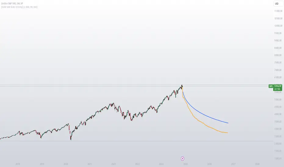
[SGM VaR Stats VS Empirical]Main Functions
Logarithmic Returns & Historical Data
Calculates logarithmic returns from closing prices.
Stores these returns in a dynamic array with a configurable maximum size.
Approximation of the Inverse Error Function
Uses an approximation of the erfinv function to calculate z-scores for given confidence levels.
Basic Statistics
Mean: Calculates the average of the data in the array.
Standard Deviation: Measures the dispersion of returns.
Median: Provides a more robust measure of central tendency for skewed distributions.
Z-Score: Converts a confidence level into a standard deviation multiplier.
Empirical vs. Statistical Projection
Empirical Projection
Based on the median of cumulative returns for each projected period.
Applies an adjustable confidence filter to exclude extreme values.
Statistical Projection
Relies on the mean and standard deviation of historical returns.
Incorporates a standard deviation multiplier for confidence-adjusted projections.
PolyLines (Graphs)
Generates projections visually through polylines:
Statistical Polyline (Blue): Based on traditional statistical methods.
Empirical Polyline (Orange): Derived from empirical data analysis.
Projection Customization
Maximum Data Size: Configurable limit for the historical data array (max_array_size).
Confidence Level: Adjustable by the user (conf_lvl), affects the width of the confidence bands.
Projection Length: Configurable number of projected periods (length_projection).
Key Steps
Capture logarithmic returns and update the historical data array.
Calculate basic statistics (mean, median, standard deviation).
Perform projections:
Empirical: Based on the median of cumulative returns.
Statistical: Based on the mean and standard deviation.
Visualization:
Compare statistical and empirical projections using polylines.
Utility
This script allows users to compare:
Traditional Statistical Projections: Based on mathematical properties of historical returns.
Empirical Projections: Relying on direct historical observations.
Divergence or convergence of these lines also highlights the presence of skewness or kurtosis in the return distribution.
Ideal for traders and financial analysts looking to assess an asset’s potential future performance using combined statistical and empirical approaches.
SPX Open vs SMA AlertThis indicator is specifically designed to identify the first market-relevant candle of the S&P 500 (SPX) after the market opens. The opening price of the trading day is compared to a customizable simple moving average (SMA) period. A visual marker and an alert are triggered when the opening price is above the SMA. Perfect for traders seeking early market trends or integrating automated trading strategies.
Features:
Market Open: The indicator uses the New York market open time (09:30 ET), accounting for time zones and daylight saving time changes.
Flexible Time Offset: Users can set a time offset to trigger alerts after the market opens.
Customizable SMA: The SMA period is adjustable, with a default value of 10.
Visual Representation: A step-line SMA is plotted directly on the chart with subtle transparency and clean markers.
Alert Functionality: Alerts are triggered when conditions are met (opening price > SMA).
Usage:
This indicator is ideal for identifying relevant trading signals early in the session.
Alerts can also serve as triggers for automated trading, e.g., in conjunction with the Trading Automation Toolbox.
Supports both intraday and daily charts.
Alarm Settings:
Select the appropriate symbol (e.g., SPX) and the alert condition "SPX Open > SMA10".
Trigger Settings:
Choose "Once Per Bar Close" to ensure the condition is evaluated at the end of each candle.
If you prefer to evaluate the condition immediately when it becomes true, choose "Once Per Minute".
Duration:
Set the alarm to "Open-ended" if you want it to remain active indefinitely.
Alternatively, set a specific expiration date for the alarm.

Weekly COTAdjusted COT Index
Improves upon: "COT Index Commercials vs large and small Speculators" by SystematicFutures
How: CoT Indexes are adjusted by Open Interest to normalise data over time, and threshold background colours are in-line with Larry Williams recommendations from his book.
Note: This indicator is **only** accurate on the Daily time-frame due to the mid-week release date for CoT data.
This script calculates and plots the Adjusted Commitment of Traders (COT) Index for Commercial, Large Speculator, and Retail (Small Speculator) categories.
The CoT Index is adjusted by Open Interest to normalise data through time, following the methodology of Larry Williams, providing insights into how these groups are positioned in the market with an arguably more historically accurate context.
COT Categories
-------------------
- Commercials (Producers/Hedgers): Large entities hedging against price changes in the underlying asset.
- Large Speculators (Non-commercials): Professional traders and funds speculating on price movements.
- Retail Traders (Nonreportable/Small Speculators): Small individual traders, typically less informed.
Features
----------
- Open Interest Adjustment
- The net positions for each category are normalized by Open Interest to account
for varying contract sizes.
- Customisable Look-back Period
- You can adjust the number of weeks for the index calculation to control the
historical range used for comparison.
- Thresholds for Extremes
- Upper and lower thresholds (configurable) are provided to mark overbought and
oversold conditions.
- Defaults
- Overbought: <=20
- Oversold: >= 80
- Hide Current Week Option
- Optionally hide the current week's data until market close for more accurate comparison.
- Visual Aids
- Plot the Commercials, Large Speculators, and Retail indexes, and optionally highlight extreme positioning.
Inputs
--------
- weeks
- Number of weeks for historical range comparison.
- upperExtreme and lowerExtreme
- Thresholds to identify overbought/oversold conditions (default 80/20).
- hideCurrentWeek
- Option to hide current week's data until market close.
- markExtremes
- Highlight extremes where any index crosses the upper or lower thresholds.
- Options to display or hide indexes for Commercials, Large Speculators, and Small Speculators.
Outputs
----------
- The script plots the COT Index for each of the three categories and highlights periods of extreme positioning with customisable thresholds.
Usage
-------
- This tool is useful for traders who want to track the positioning of different market participants over time.
- By identifying the extreme positions of Commercials, Large Speculators, and Retail traders, it can give insights into market sentiment and potential reversals.
- Reversals of trend can be confirmed with RSI Divergence (daily), for example
- Continuation can be confirmed with RSI overbought/oversold conditions (daily), and/or hidden RSI Hidden Divergence, for example

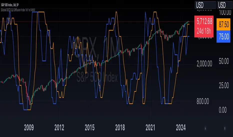
Global OECD CLI Diffusion Index YoY vs MoMThe Global OECD Composite Leading Indicators (CLI) Diffusion Index is used to gauge the health and directional momentum of the global economy and anticipate changes in economic conditions. It usually leads turning points in the economy by 6 - 9 months.
How to read: Above 50% signals economic expansion across the included countries. Below 50% signals economic contraction.
The diffusion index component specifically shows the proportion of countries with positive economic growth signals compared to those with negative or neutral signals.
The OECD CLI aggregates data from several leading economic indicators including order books, building permits, and consumer and business sentiment. It tracks the economic momentum and turning points in the business cycle across 38 OECD member countries and several other Non-OECD member countries.
Linear Regression Channel UltimateKey Features and Benefits
Logarithmic scale option for improved analysis of long-term trends and volatile markets
Activity-based profiling using either touch count or volume data
Customizable channel width and number of profile fills
Adjustable number of most active levels displayed
Highly configurable visual settings for optimal chart readability
Why Logarithmic Scale Matters
The logarithmic scale option is a game-changer for analyzing assets with exponential growth or high volatility. Unlike linear scales, log scales represent percentage changes consistently across the price range. This allows for:
Better visualization of long-term trends
More accurate comparison of price movements across different price levels
Improved analysis of volatile assets or markets experiencing rapid growth
How It Works
The indicator calculates a linear regression line based on the specified period
Upper and lower channel lines are drawn at a customizable distance from the regression line
The space between the channel lines is divided into a user-defined number of levels
For each level, the indicator tracks either:
- The number of times price touches the level (touch count method)
- The total volume traded when price is at the level (volume method)
The most active levels are highlighted based on this activity data
Understanding Touch Count vs Volume
Touch count method: Useful for identifying key support/resistance levels based on price action alone
Volume method: Provides insight into levels where the most trading activity occurs, potentially indicating stronger support/resistance
Practical Applications
Trend identification and strength assessment
Support and resistance level discovery
Entry and exit point optimization
Volume profile analysis for improved market structure understanding
This Linear Regression Channel indicator combines powerful statistical analysis with flexible visualization options, making it an invaluable tool for traders and analysts across various timeframes and markets. Its unique features, especially the logarithmic scale and activity profiling, provide deeper insights into market behavior and potential turning points.
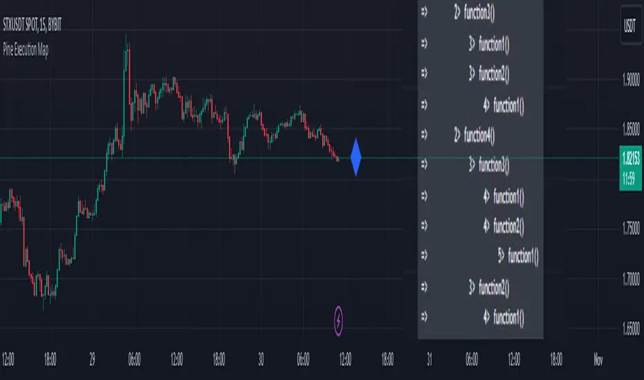
Pine Execution MapPine Script Execution Map
Overview:
This is an educational script for Pine Script developers. The script includes data structure, functions/methods, and process to capture and print Pine Script execution map of functions called while pine script execution.
Map of execution is produced for last/latest candle execution.
The script also has example code to call execution map methods and generate Pine Execution map.
Use cases:
Pine script developers can get view of how the functions are called
This can also be used while debugging the code and know which functions are called vs what developer expect code to do
One can use this while using any of the open source published script and understand how public script is organized and how functions of the script are called.
Code components:
User defined type
type EMAP
string group
string sub_group
int level
array emap = array.new()
method called internally by other methods to generate level of function being executed
method id(string tag) =>
if(str.startswith(tag, "MAIN"))
exe_level.set(0, 0)
else if(str.startswith(tag, "END"))
exe_level.set(0, exe_level.get(0) - 1)
else
exe_level.set(0, exe_level.get(0) + 1)
exe_level.get(0)
Method called from main/global scope to record execution of main scope code. There should be only one call to this method at the start of global scope.
method main(string tag) =>
this = EMAP.new()
this.group := "MAIN"
this.sub_group := tag
this.level := "MAIN".id()
emap.push(this)
Method called from main/global scope to record end of execution of main scope code. There should be only one call to this method at the end of global scope.
method end_main(string tag) =>
this = EMAP.new()
this.group := "END_MAIN"
this.sub_group := tag
this.level := 0
emap.push(this)
Method called from start of each function to record execution of function code
method call(string tag) =>
this = EMAP.new()
this.group := "SUB"
this.sub_group := tag
this.level := "SUB".id()
emap.push(this)
Method called from end of each function to record end of execution of function code
method end_call(string tag) =>
this = EMAP.new()
this.group := "END_SUB"
this.sub_group := tag
this.level := "END_SUB".id()
emap.push(this)
Pine code which generates execution map and show it as a label tooltip.
if(barstate.islast)
for rec in emap
if(not str.startswith(rec.group, "END"))
lvl_tab = str.repeat("", rec.level+1, "\t")
txt = str.format("=> {0} {1}> {2}", lvl_tab, rec.level, rec.sub_group)
debug.log(txt)
debug.lastr()
Snapshot 1:
This is the output of the script and can be viewed by hovering mouse pointer over the blue color diamond shaped label
Snapshot 2:
How to read the Pine execution map
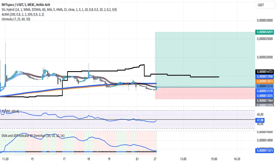
EMA and ATR Indicator BY DemirkanEMA 10 and ATR Indicator BY Demirkan
The EMA 10 and ATR Indicator combines two powerful technical indicators used to analyze trends and identify potential trading opportunities.
Indicator Components:
Exponential Moving Average (EMA):
EMA 10: Calculates the weighted average of the last 10 closing prices. This indicator is effective in tracking short-term price movements. When the price is above the EMA, it is considered that the trend is upward; when it is below, it is assessed as a downward trend.
Average True Range (ATR):
ATR: A measure of market volatility. When the ATR value falls within a specified range (between 10 and 14 in this indicator), the price movement is considered significant. This helps you base your trading decisions on more solid grounds.
Usage Recommendations:
Buy Signal: When the price is above the EMA and the ATR is within the specified range, this can be interpreted as a potential buy signal.
Sell Signal: When the price is below the EMA, this can be interpreted as a potential sell signal.
Chart Displays:
EMA Line: Displayed as a blue line, allowing you to see how the EMA relates to current price levels.
Price Status: Circles are used to indicate whether the price is above or below the EMA. A green circle indicates the price is above the EMA, while a red circle indicates it is below.
Background Colors: The chart background changes to green or red to highlight buy and sell conditions.
Aesthetic Presentation:
Using the "Flag" and "Below" parameters for the Price vs EMA indicator provides an aesthetically pleasing appearance on the chart. This type of visual presentation helps users quickly and easily grasp trading signals. Additionally, this aesthetic touch makes investors' charts look more professional and appealing.
This indicator is a useful tool for traders looking to develop short-term trading strategies. However, it should always be used in conjunction with additional analysis and other indicators.
Note: This indicator is for educational purposes only and should not be taken as investment advice.
30D Vs 90D Historical VolatilityVolatility equals risk for an underlying asset's price meaning bullish volatility is bearish for prices while bearish volatility is bullish. This compares 30-Day Historical Volatility to 90-Day Historical Volatility.
When the 30-Day crosses under the 90-day, this is typically when asset prices enter a bullish trend.
Conversely, When the 30-Day crosses above the 90-Day, this is when asset prices enter a bearish trend.
Peaks in volatility are bullish divergences while troughs are bearish divergences.

Range Detection [No Repaint]DETECTS RANGE EARLY
Using Confirmed Data:
All calculations now use to reference the previous completed candle
Signals are only generated based on completed candles
Range state is stored and confirmed before displaying
Key Changes to Prevent Repainting:
ATR calculations use previous candle data
Bollinger Bands calculate from previous closes
Price range checks use previous highs and lows
Range state is confirmed before displaying
How to Verify No Repainting:
Signals will only appear after a candle closes
Historical signals will remain unchanged
Alerts will only trigger on confirmed changes
This means:
The indicator will be slightly delayed (one candle)
But signals will be more reliable
Historical analysis will be accurate
Backtesting results will match real-time performance
Usage Tips with No-Repaint Version:
Wait for candle close before acting on signals
Use the confirmed range state for decision making
Consider the one-candle delay in your strategy timing
Alerts will only trigger on confirmed condition changes
Would you like me to:
Add a parameter to choose between real-time and no-repaint modes?
Add visual indicators for pending vs confirmed signals?
Modify the sensitivity of the range detection?