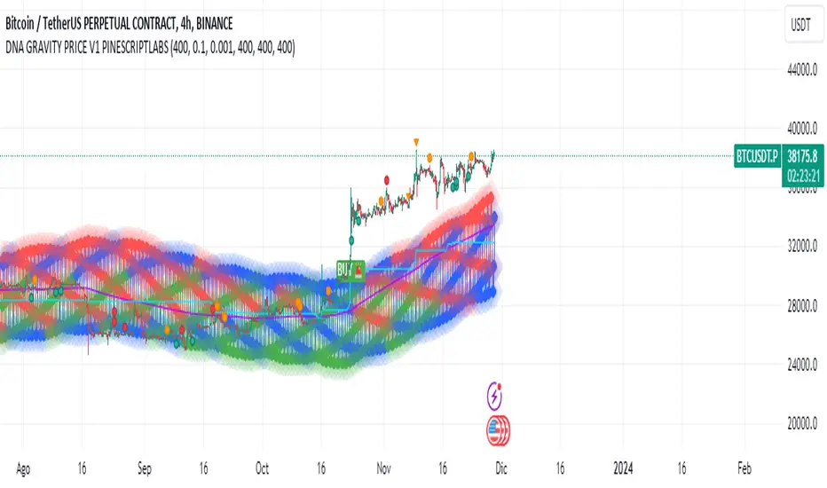
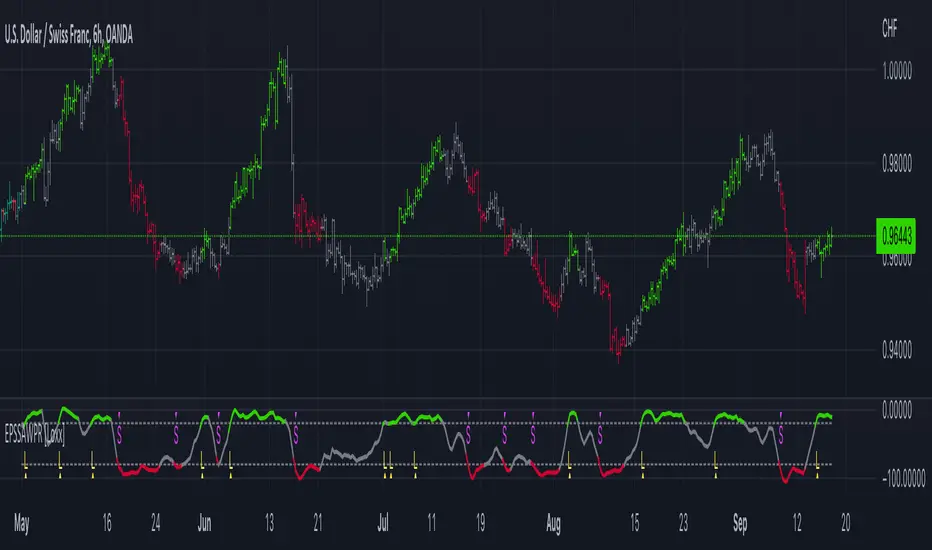
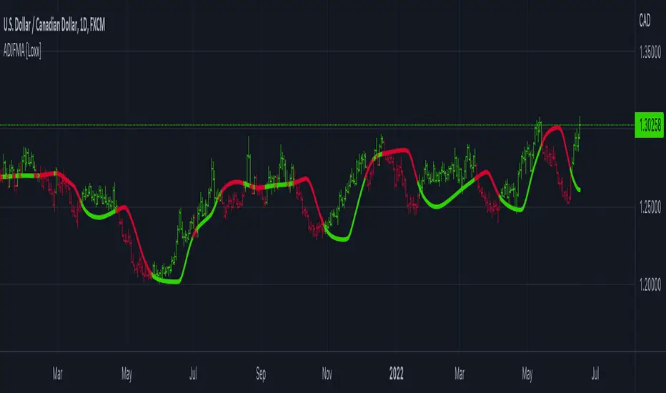
DNA GRAVITY PRICE V1 PINESCRIPTLABSWe can observe that this indicator displays the range within which the asset fluctuates around the average price, and its behavior depends on the parameters of amplitude and angular frequency. "price_mas" is a measure calculated as part of the indicator. It is derived by adding an adjusted amplitude (A_mas) multiplied by the cosine of the combination of angular frequency (w), time, and a phase shift (phi) to the average price (P0). This calculated value oscillates around the actual asset price and is used to identify potential turning points and the range where the price has established itself within the specified lookback period.
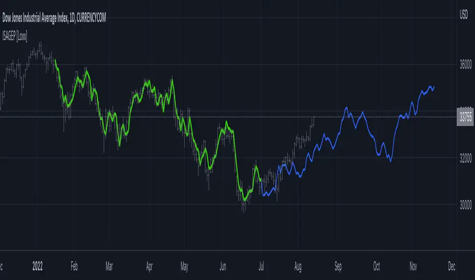
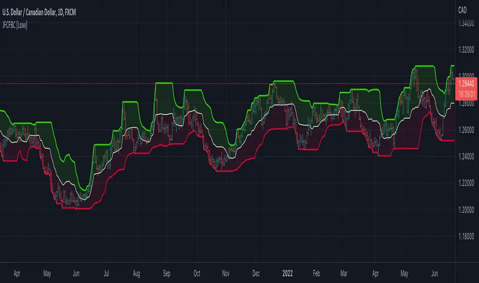
2.- At its core, the indicator utilizes the innovative concept of 'price_mas,' a calculated metric visualized in three essential colors: green to indicate low levels, blue for medium levels, and red for high levels. These colors reflect the position of the price in relation to a range determined by historical highs and lows.
In the context of the "DNA GRAVITY PRICE V1 " indicator, low, medium, and high levels specifically refer to the calculated value of 'price_mas,' which is a derived measure within the indicator. They do not directly refer to the actual asset price but rather to a calculated value that the indicator uses to analyze and predict the behavior of the asset's price.
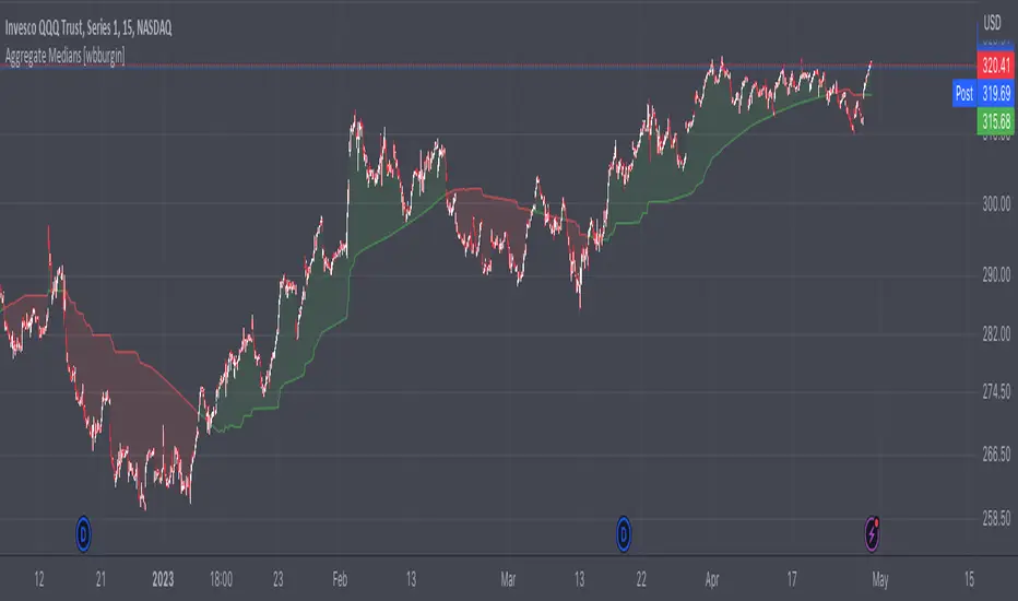
This algorithm stands out for its ability to capture the 'strength' of the price through the 'price_mas' zones. Once the price exits the zones marked by the 'price_mas' (red, blue, and green plots), it tends to return with significant force.
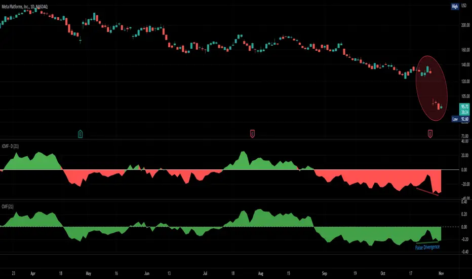
Buy & Sell Signals:
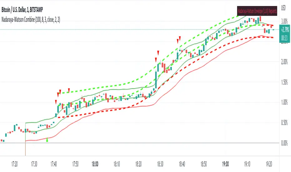
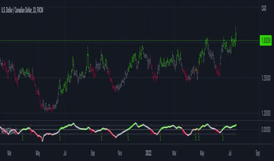
Buy Signal: If the price and the Donchian lines cross above the high threshold, visually represented by red diamonds, it indicates a strong bullish momentum. This not only shows that the price is rising but also that the trend is strong enough to push the Donchian lines, which represent price extremes over a certain period, above the threshold. This convergence of movements, marked by the crossing over the red diamonds, suggests a higher probability of the bullish trend continuing.
Sell Signal: Similarly, if the price and the Donchian lines fall below the low threshold, visualized as green diamonds, this signals a significant bearish momentum. The simultaneous decline of the price and the Donchian lines below this threshold, marked by the green diamonds, indicates that not only is the price decreasing, but the bearish trend is strong enough to influence the price extremes calculated by the Donchian lines.
Configuration:
-The "Initial Dynamic Length of MAS Price" parameter controls the smoothness and sensitivity of the indicator. A high value smooths the Simple Moving Average (SMA), making the indicator less responsive to short-term price fluctuations. On the other hand, a low value makes the indicator more sensitive to short-term price fluctuations, generating faster and more volatile signals
-This parameter, "MAS Amplitude Percentage," determines the amplitude as a percentage. Increasing the Initial Dynamic Price will result in a larger amplitude relative to the price, leading to wider ranges for the indicator. Decreasing this value will have the opposite effect, reducing the amplitude relative to the price. Increasing "A_mas_pct" can make signals more extreme and less frequent, while decreasing it will make signals smoother and more frequent.
-This parameter, "Angular Frequency of MAS," affects the frequency of oscillations in the calculation of the "Initial Dynamic Price." A higher value of "w" will make the oscillations faster and more frequent, which means that the indicator will be more responsive to abrupt price changes. Conversely, a lower value will make the oscillations slower and smoother, making the indicator less sensitive to rapid price changes. Modifying ""Angular Frequency of MAS,"" directly impacts the frequency of oscillations in the indicator.
Español:
Podemos observar que este indicador muestra el rango en el cual el activo fluctúa alrededor del precio promedio y su comportamiento depende de los parámetros de amplitud y frecuencia angular. "price_mas" es una medida calculada como parte del indicador. Se deriva al sumar una amplitud ajustada (A_mas) multiplicada por el coseno de la combinación de frecuencia angular (w), tiempo y un desplazamiento de fase (phi) al precio promedio (P0). Este valor calculado oscila alrededor del precio real del activo y se utiliza para identificar posibles puntos de giro y el rango donde el precio se ha establecido dentro del período de búsqueda especificado.
En su núcleo, el indicador utiliza el innovador concepto de 'price_mas', una métrica calculada visualizada en tres colores esenciales: verde para indicar niveles bajos, azul para niveles medios y rojo para niveles altos. Estos colores reflejan la posición del precio en relación con un rango determinado por los máximos y mínimos históricos.
En el contexto del indicador "DNA GRAVITY PRICE V1", los niveles bajos, medios y altos se refieren específicamente al valor calculado de 'price_mas', que es una medida derivada dentro del indicador. No se refieren directamente al precio real del activo, sino a un valor calculado que el indicador utiliza para analizar y predecir el comportamiento del precio del activo.
Este algoritmo se destaca por su capacidad para capturar la 'fortaleza' del precio a través de las zonas de 'price_mas'. Una vez que el precio sale de las zonas marcadas por 'price_mas' (trazas rojas, azules y verdes), tiende a regresar con una fuerza significativa. Este comportamiento es crucial para los operadores, ya que proporciona oportunidades tanto para capitalizar las retracciones de precios como para anticipar posibles cambios de tendencia.
Señales de Compra y Venta:
Señal de Compra: Si el precio y las líneas Donchian cruzan por encima del umbral alto, visualmente representado por diamantes rojos, indica un fuerte impulso alcista. Esto no solo muestra que el precio está aumentando, sino que la tendencia es lo suficientemente fuerte como para empujar las líneas Donchian, que representan los extremos de precio durante un período determinado, por encima del umbral. Esta convergencia de movimientos, marcada por el cruce sobre los diamantes rojos, sugiere una mayor probabilidad de que la tendencia alcista continúe.
Señal de Venta: De manera similar, si el precio y las líneas Donchian caen por debajo del umbral bajo, visualizado como diamantes verdes, esto señala un fuerte impulso bajista. La caída simultánea del precio y las líneas Donchian por debajo de este umbral, marcada por los diamantes verdes, indica que no solo el precio está disminuyendo, sino que la tendencia bajista es lo suficientemente fuerte como para influir en los extremos de precio calculados por las líneas Donchian.
Configuración:
El parámetro "Longitud Dinámica Inicial de MAS Price" controla la suavidad y la sensibilidad del indicador. Un valor alto suaviza el Promedio Móvil Simple (SMA), lo que hace que el indicador sea menos sensible a las fluctuaciones de precio a corto plazo. Por otro lado, un valor bajo hace que el indicador sea más sensible a las fluctuaciones de precio a corto plazo, generando señales más rápidas y volátiles.
Este parámetro, "Porcentaje de Amplitud de MAS," determina la amplitud como un porcentaje. Aumentar el valor de "Longitud Dinámica Inicial de MAS Price" dará como resultado una amplitud más grande en relación con el precio, lo que conducirá a rangos más amplios para el indicador. Disminuir este valor tendrá el efecto contrario, reduciendo la amplitud en relación con el precio. Aumentar "Porcentaje de A_mas" puede hacer que las señales sean más extremas y menos frecuentes, mientras que disminuirlo hará que las señales sean más suaves y más frecuentes.
Este parámetro, "Frecuencia Angular de MAS," afecta la frecuencia de las oscilaciones en el cálculo del "Precio Móvil Simple Inicial." Un valor más alto de "w" hará que las oscilaciones sean más rápidas y frecuentes, lo que significa que el indicador será más receptivo a cambios abruptos en el precio. Por otro lado, un valor más bajo hará que las oscilaciones sean más lentas y suaves, haciendo que el indicador sea menos sensible a cambios rápidos en el precio. Modificar "Frecuencia Angular de MAS" afecta directamente la frecuencia de las oscilaciones en el indicador.
Penunjuk Pine Script®