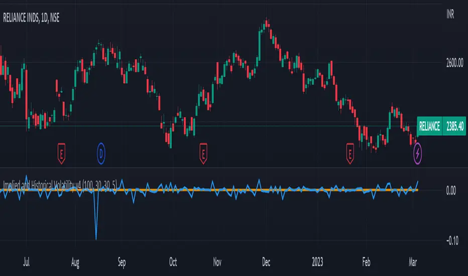
Implied and Historical Volatility v4There is a famous option strategy📊 played on volatility📈. Where people go short on volatility, generally, this strategy is used before any significant event or earnings release. The basic phenomenon is that the Implied Volatility shoots up before the event and drops after the event, while the volatility of the security does not increase in most of the scenarios. 💹
I have tried to create an Indicator using which you
can analyse the historical change in Implied Volatility Vs Historic Volatility.
To get a basic idea of how the security moved during different events.
Notes:
a) Implied Volatility is calculated using the bisection method and Black 76 model option pricing model.
b) For the risk-free rate I have fetched the price of the “10-Year Indian Government Bond” price and calculated its yield to be used as our Risk-Free rate.
Cari dalam skrip untuk "implied"
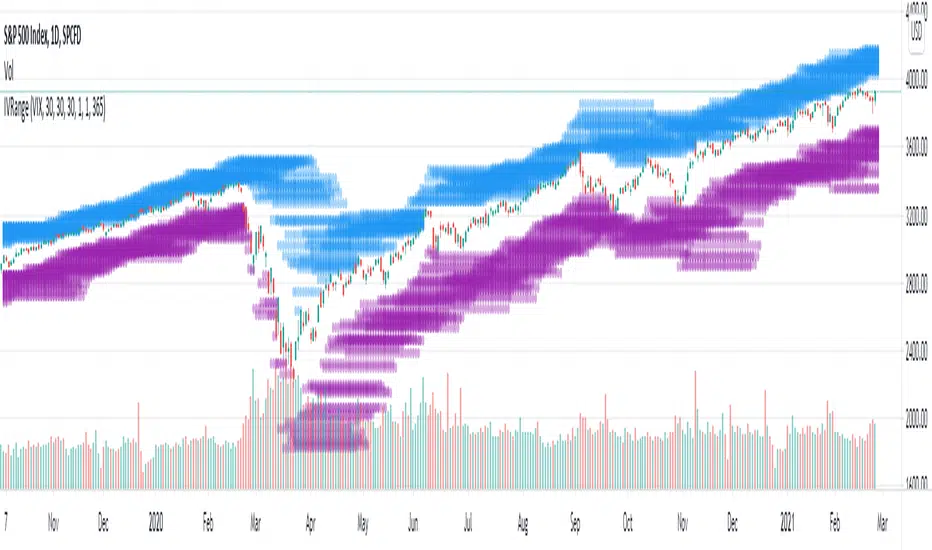
Implied Volatility Range ProjectionThis script plots an expected future range estimation based on implied volatilities, using a specified volatility index as proxy for ATM implied volatilities.
For example the S&P 500 could use the VIX.
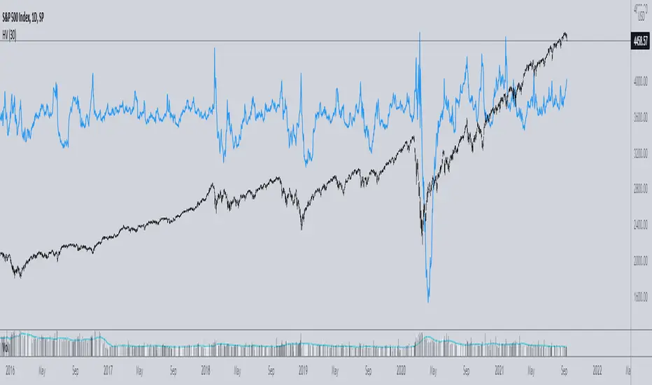
Implied minus Historical VolatilityJust a simple comparison of 30 day historical volatility versus 30 day implied volatility(VIX). In general, when VIX is way above realized or historical Vol, in general that is quite bullish. Backtest will be available soon.
Synthetic Implied APROverview
The Synthetic Implied APR is an artificial implied APR, designed to imitate the implied APR seen when trading cryptocurrency funding rates. It combines real-time funding rates with premium data to calculate an artificial market expectation of the annualized funding rate.
The (actual) implied APR is the market's expectation of the annualized funding rate. This is dependent on bid/ask impacts of the implied APR, something which is currently unavailable to fetch with TradingView. In essence, an implied APR of X% means traders believe that asset's funding fees to average X% when annualized.
What's important to understand, is that the actual value of the synthetic implied APR is not relevant. We only simply use its relative changes when we trade (i.e if it crosses above/below its MA for a given weight). Even for the same asset, the implied APRs will change depending on days to maturity.
How it calculates
The synthetic implied APR is calculated with these steps:
Collects premium data from perpetual futures markets using optimized lower timeframe requests (check my 'Predicted Funding Rates' indicator)
Calculates the funding rate by adding the premium to an interest rate component (clamped within exchange limits)
Derives the underlying APR from the 8-hour funding rate (funding rate × 3 × 365)
Apply a weighed formula that imitates both the direction (underlying APR) with the volatility of prices (from the premium index and funding)
premium_component = (prem_avg / 50 ) * 365
weighedprem = (weight * fr) + ((1 - weight) * apr) + (premium_component * 0.3)
impliedAPR = math.avg(weighedprem, ta.sma(apr, maLength))
How to use it: Generally
Preface: Funding rates are an indication of market sentiment
If funding is positive, generally the market is bullish as longs are willing to pay shorts funding
If funding is negative, generally the market is bearish as shorts are willing to pay longs funding
So, this script can be used like a typical oscillator:
Bullish: If implied APR > MA OR if implied APR MA is green
Bearish: If implied APR < MA OR if implied APR MA is red
The components:
Synthetic Implied APR: The main metric. At current setting of 0.7, it imitates volatility
Weight: The higher the value, the smoother the synthetic implied APR is (and MA too). This value is very important to the imitation. At 0.7, it imitates the actual volatility of the implied APR. At weight = 1, it becomes very smooth. Perfect for trading
Synthetic Implied APR Moving Average: A moving average of the Synthetic implied APR. Can choose from multiple selections, (SMA, EMA, WMA, HMA, VWMA, RMA)
How to use it: Trading Funding
When trading funding there're multiple ways to use it with different settings
Trade funding rates with trend changes
Settings: Weight = 1
Method 1: When the implied APR MA turns green, long funding rates (or short if red)
Method 2: When the implied APR crosses above the MA, long funding rates (or short when crosses below)
Trade funding rates with MA pullbacks
Settings: Weight = 0.7, timeframe 15m
In an uptrend: When implied APR crosses below then above the script, long funding opportunity
In an downtrend: When implied APR crosses above then below the script, shortfunding opportunity
You can determine the trend with the method before, using a weight of 1
To trade funding rates, it's best to have these 3 scripts at these settings:
Predicted Funding Rates: This allows you to see the predicted funding rates and see if they've maxxed out for added confluence too (+/-0.01% usually for Binance BTC futures)
Synthetic implied APR: At weight 1, the MA provides a good trend (whether close above/below or colour change)
Synthetic implied APR: At weight 0.7, it provides a good imitation of volatility
How to use it: Trading Futures
When trading futures:
You can determine roughly what the trend is, if the assumption is made that funding rates can help identify trends if used as a sentiment indicator. It should be supplemented with traditional trend trading methods
To prevent whipsaws, weight should remain high
Long trend: When the implied APR MA turns green OR when it crosses above its MA
Short trend: When the implied APR MA turns red OR when it below above its MA
Why it's original
This indicator introduces a unique synthetic weighting system that combines funding rates, underlying APR, and premium components in a way not found in existing TradingView scripts. Trading funding rates is a niche area, there aren't that many scripts currently available. And to my knowledge, there's no synthetic implied APR scripts available on TradingView either. So I believe this script to be original in that sense.
Notes
Because it depends on my triangular weighting algos, optimal accuracy is found on timeframes that are 4H or less. On higher timeframes, the accuracy drops off. Best timeframes for intraday trading using this are 15m or 1 hour
The higher the timeframe, the lower the MA one should use. At 1 hour, 200 or higher is best. At say, 4h, length of 50 is best
Only works for coins that have a Binance premium index
Inputs
Funding Period - Select between "1 Hour" or "8 Hour" funding cycles. 8 hours is standard for Binance
Table - Toggle the information dashboard on/off to show or hide real-time metrics including funding rate, premium, and APR value
Weight - Controls the balance between funding rate (higher values = smoother) and APR (lower values = more responsive) in the calculation, ranging from 0.0 to 1.0. Default is 0.7, this imitates the volatility
Auto Timeframe Implied Length - Automatically calculates optimal smoothing length based on your chart timeframe for consistent behavior across different time periods
Manual Implied Length - Sets a fixed smoothing length (in bars) when auto mode is disabled, with lower values being more responsive and higher values being smoother
Show Implied APR MA - Displays an additional moving average line of the Synthetic Implied APR to help identify trend direction and crossover signals
MA Type for Implied APR - Selects the calculation method (SMA, EMA, WMA, HMA, VWMA, or RMA) for the moving average, each offering different responsiveness and lag characteristics
MA Length for Implied APR - Sets the lookback period (1-500 bars) for the moving average, with shorter lengths providing more signals and longer lengths filtering noise
Show Underlying APR - Displays the raw APR calculation (without synthetic weighting) as a reference line to compare against the main indicator
Bullish Color - Sets the color for positive values in the table and rising MA line
Bearish Color - Sets the color for negative values in the table and falling MA line
Table Background - Customizes the background color and transparency of the information dashboard
Table Text Color - Sets the color for label text in the left column of the information table
Table Text Size - Controls the font size of table text with options from Tiny to Huge

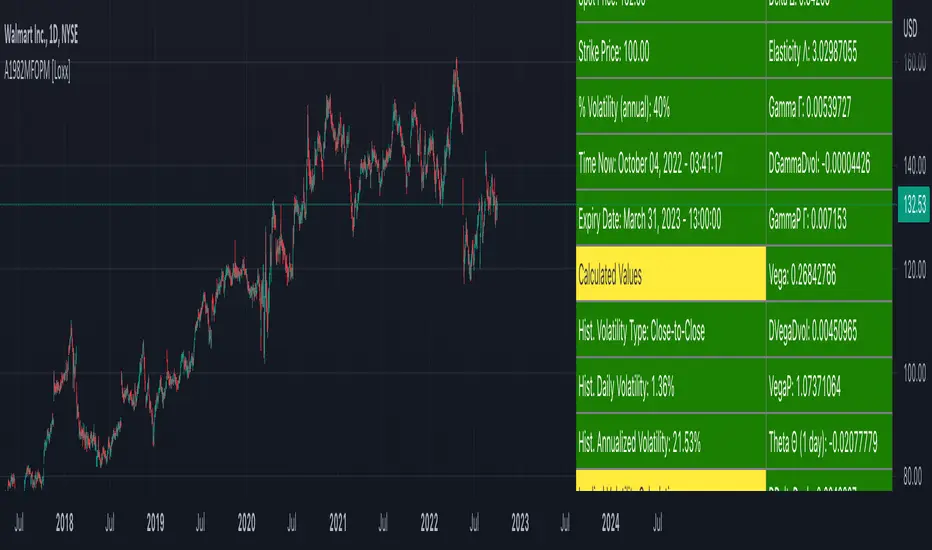
Asay (1982) Margined Futures Option Pricing Model [Loxx]Asay (1982) Margined Futures Option Pricing Model is an adaptation of the Black-Scholes-Merton Option Pricing Model including Analytical Greeks and implied volatility calculations. The following information is an excerpt from Espen Gaarder Haug's book "Option Pricing Formulas". This version is to price Options on Futures where premium is fully margined. This means the Risk-free Rate, dividend, and cost to carry are all zero. The options sensitivities (Greeks) are the partial derivatives of the Black-Scholes-Merton ( BSM ) formula. Analytical Greeks for our purposes here are broken down into various categories:
Delta Greeks: Delta, DDeltaDvol, Elasticity
Gamma Greeks: Gamma, GammaP, DGammaDvol, Speed
Vega Greeks: Vega , DVegaDvol/Vomma, VegaP
Theta Greeks: Theta
Probability Greeks: StrikeDelta, Risk Neutral Density
(See the code for more details)
Black-Scholes-Merton Option Pricing
The Black-Scholes-Merton model can be "generalized" by incorporating a cost-of-carry rate b. This model can be used to price European options on stocks, stocks paying a continuous dividend yield, options on futures , and currency options:
c = S * e^((b - r) * T) * N(d1) - X * e^(-r * T) * N(d2)
p = X * e^(-r * T) * N(-d2) - S * e^((b - r) * T) * N(-d1)
where
d1 = (log(S / X) + (b + v^2 / 2) * T) / (v * T^0.5)
d2 = d1 - v * T^0.5
b = r ... gives the Black and Scholes (1973) stock option model.
b = r — q ... gives the Merton (1973) stock option model with continuous dividend yield q.
b = 0 ... gives the Black (1976) futures option model.
b = 0 and r = 0 ... gives the Asay (1982) margined futures option model. <== this is the one used for this indicator!
b = r — rf ... gives the Garman and Kohlhagen (1983) currency option model.
Inputs
S = Stock price.
X = Strike price of option.
T = Time to expiration in years.
r = Risk-free rate
d = dividend yield
v = Volatility of the underlying asset price
cnd (x) = The cumulative normal distribution function
nd(x) = The standard normal density function
convertingToCCRate(r, cmp ) = Rate compounder
gImpliedVolatilityNR(string CallPutFlag, float S, float x, float T, float r, float b, float cm , float epsilon) = Implied volatility via Newton Raphson
gBlackScholesImpVolBisection(string CallPutFlag, float S, float x, float T, float r, float b, float cm ) = implied volatility via bisection
Implied Volatility: The Bisection Method
The Newton-Raphson method requires knowledge of the partial derivative of the option pricing formula with respect to volatility ( vega ) when searching for the implied volatility . For some options (exotic and American options in particular), vega is not known analytically. The bisection method is an even simpler method to estimate implied volatility when vega is unknown. The bisection method requires two initial volatility estimates (seed values):
1. A "low" estimate of the implied volatility , al, corresponding to an option value, CL
2. A "high" volatility estimate, aH, corresponding to an option value, CH
The option market price, Cm , lies between CL and cH . The bisection estimate is given as the linear interpolation between the two estimates:
v(i + 1) = v(L) + (c(m) - c(L)) * (v(H) - v(L)) / (c(H) - c(L))
Replace v(L) with v(i + 1) if c(v(i + 1)) < c(m), or else replace v(H) with v(i + 1) if c(v(i + 1)) > c(m) until |c(m) - c(v(i + 1))| <= E, at which point v(i + 1) is the implied volatility and E is the desired degree of accuracy.
Implied Volatility: Newton-Raphson Method
The Newton-Raphson method is an efficient way to find the implied volatility of an option contract. It is nothing more than a simple iteration technique for solving one-dimensional nonlinear equations (any introductory textbook in calculus will offer an intuitive explanation). The method seldom uses more than two to three iterations before it converges to the implied volatility . Let
v(i + 1) = v(i) + (c(v(i)) - c(m)) / (dc / dv (i))
until |c(m) - c(v(i + 1))| <= E at which point v(i + 1) is the implied volatility , E is the desired degree of accuracy, c(m) is the market price of the option, and dc/ dv (i) is the vega of the option evaluaated at v(i) (the sensitivity of the option value for a small change in volatility ).
Things to know
Only works on the daily timeframe and for the current source price.
You can adjust the text size to fit the screen
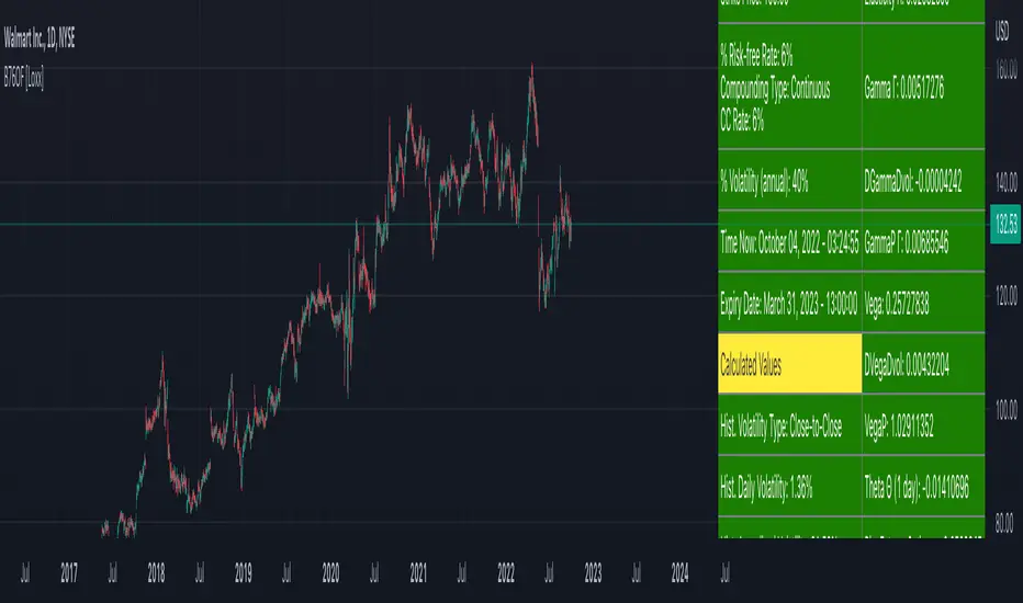
Black-76 Options on Futures [Loxx]Black-76 Options on Futures is an adaptation of the Black-Scholes-Merton Option Pricing Model including Analytical Greeks and implied volatility calculations. The following information is an excerpt from Espen Gaarder Haug's book "Option Pricing Formulas". This version is to price Options on Futures. The options sensitivities (Greeks) are the partial derivatives of the Black-Scholes-Merton ( BSM ) formula. Analytical Greeks for our purposes here are broken down into various categories:
Delta Greeks: Delta, DDeltaDvol, Elasticity
Gamma Greeks: Gamma, GammaP, DGammaDvol, Speed
Vega Greeks: Vega , DVegaDvol/Vomma, VegaP
Theta Greeks: Theta
Rate/Carry Greeks: Rho futures option
Probability Greeks: StrikeDelta, Risk Neutral Density
(See the code for more details)
Black-Scholes-Merton Option Pricing
The Black-Scholes-Merton model can be "generalized" by incorporating a cost-of-carry rate b. This model can be used to price European options on stocks, stocks paying a continuous dividend yield, options on futures , and currency options:
c = S * e^((b - r) * T) * N(d1) - X * e^(-r * T) * N(d2)
p = X * e^(-r * T) * N(-d2) - S * e^((b - r) * T) * N(-d1)
where
d1 = (log(S / X) + (b + v^2 / 2) * T) / (v * T^0.5)
d2 = d1 - v * T^0.5
b = r ... gives the Black and Scholes (1973) stock option model.
b = r — q ... gives the Merton (1973) stock option model with continuous dividend yield q.
b = 0 ... gives the Black (1976) futures option model. <== this is the one used for this indicator!
b = 0 and r = 0 ... gives the Asay (1982) margined futures option model.
b = r — rf ... gives the Garman and Kohlhagen (1983) currency option model.
Inputs
S = Stock price.
X = Strike price of option.
T = Time to expiration in years.
r = Risk-free rate
d = dividend yield
v = Volatility of the underlying asset price
cnd (x) = The cumulative normal distribution function
nd(x) = The standard normal density function
convertingToCCRate(r, cmp ) = Rate compounder
gImpliedVolatilityNR(string CallPutFlag, float S, float x, float T, float r, float b, float cm , float epsilon) = Implied volatility via Newton Raphson
gBlackScholesImpVolBisection(string CallPutFlag, float S, float x, float T, float r, float b, float cm ) = implied volatility via bisection
Implied Volatility: The Bisection Method
The Newton-Raphson method requires knowledge of the partial derivative of the option pricing formula with respect to volatility ( vega ) when searching for the implied volatility . For some options (exotic and American options in particular), vega is not known analytically. The bisection method is an even simpler method to estimate implied volatility when vega is unknown. The bisection method requires two initial volatility estimates (seed values):
1. A "low" estimate of the implied volatility , al, corresponding to an option value, CL
2. A "high" volatility estimate, aH, corresponding to an option value, CH
The option market price, Cm , lies between CL and cH . The bisection estimate is given as the linear interpolation between the two estimates:
v(i + 1) = v(L) + (c(m) - c(L)) * (v(H) - v(L)) / (c(H) - c(L))
Replace v(L) with v(i + 1) if c(v(i + 1)) < c(m), or else replace v(H) with v(i + 1) if c(v(i + 1)) > c(m) until |c(m) - c(v(i + 1))| <= E, at which point v(i + 1) is the implied volatility and E is the desired degree of accuracy.
Implied Volatility: Newton-Raphson Method
The Newton-Raphson method is an efficient way to find the implied volatility of an option contract. It is nothing more than a simple iteration technique for solving one-dimensional nonlinear equations (any introductory textbook in calculus will offer an intuitive explanation). The method seldom uses more than two to three iterations before it converges to the implied volatility . Let
v(i + 1) = v(i) + (c(v(i)) - c(m)) / (dc / dv (i))
until |c(m) - c(v(i + 1))| <= E at which point v(i + 1) is the implied volatility , E is the desired degree of accuracy, c(m) is the market price of the option, and dc/ dv (i) is the vega of the option evaluaated at v(i) (the sensitivity of the option value for a small change in volatility ).
Things to know
Only works on the daily timeframe and for the current source price.
You can adjust the text size to fit the screen
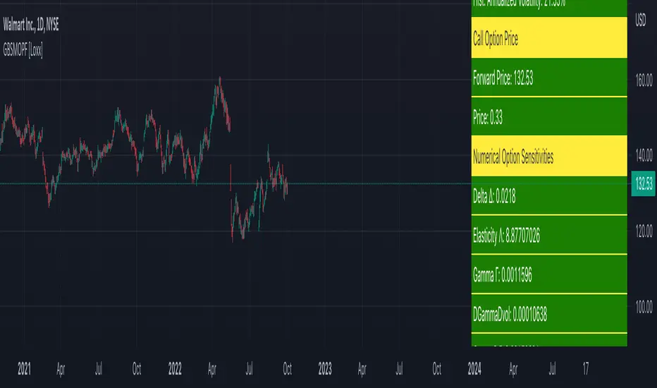
Garman and Kohlhagen (1983) for Currency Options [Loxx]Garman and Kohlhagen (1983) for Currency Options is an adaptation of the Black-Scholes-Merton Option Pricing Model including Analytical Greeks and implied volatility calculations. The following information is an excerpt from Espen Gaarder Haug's book "Option Pricing Formulas". This version of BSMOPM is to price Currency Options. The options sensitivities (Greeks) are the partial derivatives of the Black-Scholes-Merton ( BSM ) formula. Analytical Greeks for our purposes here are broken down into various categories:
Delta Greeks: Delta, DDeltaDvol, Elasticity
Gamma Greeks: Gamma, GammaP, DGammaDSpot/speed, DGammaDvol/Zomma
Vega Greeks: Vega , DVegaDvol/Vomma, VegaP, Speed
Theta Greeks: Theta
Rate/Carry Greeks: Rho, Rho futures option, Carry Rho, Phi/Rho2
Probability Greeks: StrikeDelta, Risk Neutral Density
(See the code for more details)
Black-Scholes-Merton Option Pricing for Currency Options
The Garman and Kohlhagen (1983) modified Black-Scholes model can be used to price European currency options; see also Grabbe (1983). The model is mathematically equivalent to the Merton (1973) model presented earlier. The only difference is that the dividend yield is replaced by the risk-free rate of the foreign currency rf:
c = S * e^(-rf * T) * N(d1) - X * e^(-r * T) * N(d2)
p = X * e^(-r * T) * N(-d2) - S * e^(-rf * T) * N(-d1)
where
d1 = (log(S / X) + (r - rf + v^2 / 2) * T) / (v * T^0.5)
d2 = d1 - v * T^0.5
For more information on currency options, see DeRosa (2000)
Inputs
S = Stock price.
X = Strike price of option.
T = Time to expiration in years.
r = Risk-free rate
rf = Risk-free rate of the foreign currency
v = Volatility of the underlying asset price
cnd (x) = The cumulative normal distribution function
nd(x) = The standard normal density function
convertingToCCRate(r, cmp ) = Rate compounder
gImpliedVolatilityNR(string CallPutFlag, float S, float x, float T, float r, float b, float cm , float epsilon) = Implied volatility via Newton Raphson
gBlackScholesImpVolBisection(string CallPutFlag, float S, float x, float T, float r, float b, float cm ) = implied volatility via bisection
Implied Volatility: The Bisection Method
The Newton-Raphson method requires knowledge of the partial derivative of the option pricing formula with respect to volatility ( vega ) when searching for the implied volatility . For some options (exotic and American options in particular), vega is not known analytically. The bisection method is an even simpler method to estimate implied volatility when vega is unknown. The bisection method requires two initial volatility estimates (seed values):
1. A "low" estimate of the implied volatility , al, corresponding to an option value, CL
2. A "high" volatility estimate, aH, corresponding to an option value, CH
The option market price, Cm , lies between CL and cH . The bisection estimate is given as the linear interpolation between the two estimates:
v(i + 1) = v(L) + (c(m) - c(L)) * (v(H) - v(L)) / (c(H) - c(L))
Replace v(L) with v(i + 1) if c(v(i + 1)) < c(m), or else replace v(H) with v(i + 1) if c(v(i + 1)) > c(m) until |c(m) - c(v(i + 1))| <= E, at which point v(i + 1) is the implied volatility and E is the desired degree of accuracy.
Implied Volatility: Newton-Raphson Method
The Newton-Raphson method is an efficient way to find the implied volatility of an option contract. It is nothing more than a simple iteration technique for solving one-dimensional nonlinear equations (any introductory textbook in calculus will offer an intuitive explanation). The method seldom uses more than two to three iterations before it converges to the implied volatility . Let
v(i + 1) = v(i) + (c(v(i)) - c(m)) / (dc / dv (i))
until |c(m) - c(v(i + 1))| <= E at which point v(i + 1) is the implied volatility , E is the desired degree of accuracy, c(m) is the market price of the option, and dc/ dv (i) is the vega of the option evaluaated at v(i) (the sensitivity of the option value for a small change in volatility ).
Things to know
Only works on the daily timeframe and for the current source price.
You can adjust the text size to fit the screen
Related indicators:
BSM OPM 1973 w/ Continuous Dividend Yield
Black-Scholes 1973 OPM on Non-Dividend Paying Stocks
Generalized Black-Scholes-Merton w/ Analytical Greeks
Generalized Black-Scholes-Merton Option Pricing Formula
Sprenkle 1964 Option Pricing Model w/ Num. Greeks
Modified Bachelier Option Pricing Model w/ Num. Greeks
Bachelier 1900 Option Pricing Model w/ Numerical Greeks

Black-Scholes 1973 OPM on Non-Dividend Paying Stocks [Loxx]Black-Scholes 1973 OPM on Non-Dividend Paying Stocks is an adaptation of the Black-Scholes-Merton Option Pricing Model including Analytical Greeks and implied volatility calculations. Making b equal to r yields the BSM model where dividends are not considered. The following information is an excerpt from Espen Gaarder Haug's book "Option Pricing Formulas". The options sensitivities (Greeks) are the partial derivatives of the Black-Scholes-Merton ( BSM ) formula. For our purposes here are, Analytical Greeks are broken down into various categories:
Delta Greeks: Delta, DDeltaDvol, Elasticity
Gamma Greeks: Gamma, GammaP, DGammaDSpot/speed, DGammaDvol/Zomma
Vega Greeks: Vega , DVegaDvol/Vomma, VegaP
Theta Greeks: Theta
Rate/Carry Greeks: Rho
Probability Greeks: StrikeDelta, Risk Neutral Density
(See the code for more details)
Black-Scholes-Merton Option Pricing
The BSM formula and its binomial counterpart may easily be the most used "probability model/tool" in everyday use — even if we con- sider all other scientific disciplines. Literally tens of thousands of people, including traders, market makers, and salespeople, use option formulas several times a day. Hardly any other area has seen such dramatic growth as the options and derivatives businesses. In this chapter we look at the various versions of the basic option formula. In 1997 Myron Scholes and Robert Merton were awarded the Nobel Prize (The Bank of Sweden Prize in Economic Sciences in Memory of Alfred Nobel). Unfortunately, Fischer Black died of cancer in 1995 before he also would have received the prize.
It is worth mentioning that it was not the option formula itself that Myron Scholes and Robert Merton were awarded the Nobel Prize for, the formula was actually already invented, but rather for the way they derived it — the replicating portfolio argument, continuous- time dynamic delta hedging, as well as making the formula consistent with the capital asset pricing model (CAPM). The continuous dynamic replication argument is unfortunately far from robust. The popularity among traders for using option formulas heavily relies on hedging options with options and on the top of this dynamic delta hedging, see Higgins (1902), Nelson (1904), Mello and Neuhaus (1998), Derman and Taleb (2005), as well as Haug (2006) for more details on this topic. In any case, this book is about option formulas and not so much about how to derive them.
Provided here are the various versions of the Black-Scholes-Merton formula presented in the literature. All formulas in this section are originally derived based on the underlying asset S follows a geometric Brownian motion
dS = mu * S * dt + v * S * dz
where t is the expected instantaneous rate of return on the underlying asset, a is the instantaneous volatility of the rate of return, and dz is a Wiener process.
The formula derived by Black and Scholes (1973) can be used to value a European option on a stock that does not pay dividends before the option's expiration date. Letting c and p denote the price of European call and put options, respectively, the formula states that
c = S * N(d1) - X * e^(-r * T) * N(d2)
p = X * e^(-r * T) * N(d2) - S * N(d1)
where
d1 = (log(S / X) + (r + v^2 / 2) * T) / (v * T^0.5)
d2 = (log(S / X) + (r - v^2 / 2) * T) / (v * T^0.5) = d1 - v * T^0.5
**This version of the Black-Scholes formula can also be used to price American call options on a non-dividend-paying stock, since it will never be optimal to exercise the option before expiration.**
Inputs
S = Stock price.
X = Strike price of option.
T = Time to expiration in years.
r = Risk-free rate
b = Cost of carry
v = Volatility of the underlying asset price
cnd (x) = The cumulative normal distribution function
nd(x) = The standard normal density function
convertingToCCRate(r, cmp ) = Rate compounder
gImpliedVolatilityNR(string CallPutFlag, float S, float x, float T, float r, float b, float cm , float epsilon) = Implied volatility via Newton Raphson
gBlackScholesImpVolBisection(string CallPutFlag, float S, float x, float T, float r, float b, float cm ) = implied volatility via bisection
Implied Volatility: The Bisection Method
The Newton-Raphson method requires knowledge of the partial derivative of the option pricing formula with respect to volatility ( vega ) when searching for the implied volatility . For some options (exotic and American options in particular), vega is not known analytically. The bisection method is an even simpler method to estimate implied volatility when vega is unknown. The bisection method requires two initial volatility estimates (seed values):
1. A "low" estimate of the implied volatility , al, corresponding to an option value, CL
2. A "high" volatility estimate, aH, corresponding to an option value, CH
The option market price, Cm , lies between CL and cH . The bisection estimate is given as the linear interpolation between the two estimates:
v(i + 1) = v(L) + (c(m) - c(L)) * (v(H) - v(L)) / (c(H) - c(L))
Replace v(L) with v(i + 1) if c(v(i + 1)) < c(m), or else replace v(H) with v(i + 1) if c(v(i + 1)) > c(m) until |c(m) - c(v(i + 1))| <= E, at which point v(i + 1) is the implied volatility and E is the desired degree of accuracy.
Implied Volatility: Newton-Raphson Method
The Newton-Raphson method is an efficient way to find the implied volatility of an option contract. It is nothing more than a simple iteration technique for solving one-dimensional nonlinear equations (any introductory textbook in calculus will offer an intuitive explanation). The method seldom uses more than two to three iterations before it converges to the implied volatility . Let
v(i + 1) = v(i) + (c(v(i)) - c(m)) / (dc / dv (i))
until |c(m) - c(v(i + 1))| <= E at which point v(i + 1) is the implied volatility , E is the desired degree of accuracy, c(m) is the market price of the option, and dc/ dv (i) is the vega of the option evaluaated at v(i) (the sensitivity of the option value for a small change in volatility ).
Things to know
Only works on the daily timeframe and for the current source price.
You can adjust the text size to fit the screen

Generalized Black-Scholes-Merton Option Pricing Formula [Loxx]Generalized Black-Scholes-Merton Option Pricing Formula is an adaptation of the Black-Scholes-Merton Option Pricing Model including Numerical Greeks aka "Option Sensitivities" and implied volatility calculations. The following information is an excerpt from Espen Gaarder Haug's book "Option Pricing Formulas".
Black-Scholes-Merton Option Pricing
The BSM formula and its binomial counterpart may easily be the most used "probability model/tool" in everyday use — even if we con- sider all other scientific disciplines. Literally tens of thousands of people, including traders, market makers, and salespeople, use option formulas several times a day. Hardly any other area has seen such dramatic growth as the options and derivatives businesses. In this chapter we look at the various versions of the basic option formula. In 1997 Myron Scholes and Robert Merton were awarded the Nobel Prize (The Bank of Sweden Prize in Economic Sciences in Memory of Alfred Nobel). Unfortunately, Fischer Black died of cancer in 1995 before he also would have received the prize.
It is worth mentioning that it was not the option formula itself that Myron Scholes and Robert Merton were awarded the Nobel Prize for, the formula was actually already invented, but rather for the way they derived it — the replicating portfolio argument, continuous- time dynamic delta hedging, as well as making the formula consistent with the capital asset pricing model (CAPM). The continuous dynamic replication argument is unfortunately far from robust. The popularity among traders for using option formulas heavily relies on hedging options with options and on the top of this dynamic delta hedging, see Higgins (1902), Nelson (1904), Mello and Neuhaus (1998), Derman and Taleb (2005), as well as Haug (2006) for more details on this topic. In any case, this book is about option formulas and not so much about how to derive them.
Provided here are the various versions of the Black-Scholes-Merton formula presented in the literature. All formulas in this section are originally derived based on the underlying asset S follows a geometric Brownian motion
dS = mu * S * dt + v * S * dz
where t is the expected instantaneous rate of return on the underlying asset, a is the instantaneous volatility of the rate of return, and dz is a Wiener process.
The formula derived by Black and Scholes (1973) can be used to value a European option on a stock that does not pay dividends before the option's expiration date. Letting c and p denote the price of European call and put options, respectively, the formula states that
c = S * N(d1) - X * e^(-r * T) * N(d2)
p = X * e^(-r * T) * N(d2) - S * N(d1)
where
d1 = (log(S / X) + (r + v^2 / 2) * T) / (v * T^0.5)
d2 = (log(S / X) + (r - v^2 / 2) * T) / (v * T^0.5) = d1 - v * T^0.5
Inputs
S = Stock price.
X = Strike price of option.
T = Time to expiration in years.
r = Risk-free rate
b = Cost of carry
v = Volatility of the underlying asset price
cnd (x) = The cumulative normal distribution function
nd(x) = The standard normal density function
convertingToCCRate(r, cmp ) = Rate compounder
gImpliedVolatilityNR(string CallPutFlag, float S, float x, float T, float r, float b, float cm, float epsilon) = Implied volatility via Newton Raphson
gBlackScholesImpVolBisection(string CallPutFlag, float S, float x, float T, float r, float b, float cm) = implied volatility via bisection
Implied Volatility: The Bisection Method
The Newton-Raphson method requires knowledge of the partial derivative of the option pricing formula with respect to volatility (vega) when searching for the implied volatility. For some options (exotic and American options in particular), vega is not known analytically. The bisection method is an even simpler method to estimate implied volatility when vega is unknown. The bisection method requires two initial volatility estimates (seed values):
1. A "low" estimate of the implied volatility, al, corresponding to an option value, CL
2. A "high" volatility estimate, aH, corresponding to an option value, CH
The option market price, Cm, lies between CL and cH. The bisection estimate is given as the linear interpolation between the two estimates:
v(i + 1) = v(L) + (c(m) - c(L)) * (v(H) - v(L)) / (c(H) - c(L))
Replace v(L) with v(i + 1) if c(v(i + 1)) < c(m), or else replace v(H) with v(i + 1) if c(v(i + 1)) > c(m) until |c(m) - c(v(i + 1))| <= E, at which point v(i + 1) is the implied volatility and E is the desired degree of accuracy.
Implied Volatility: Newton-Raphson Method
The Newton-Raphson method is an efficient way to find the implied volatility of an option contract. It is nothing more than a simple iteration technique for solving one-dimensional nonlinear equations (any introductory textbook in calculus will offer an intuitive explanation). The method seldom uses more than two to three iterations before it converges to the implied volatility. Let
v(i + 1) = v(i) + (c(v(i)) - c(m)) / (dc / dv(i))
until |c(m) - c(v(i + 1))| <= E at which point v(i + 1) is the implied volatility, E is the desired degree of accuracy, c(m) is the market price of the option, and dc/dv(i) is the vega of the option evaluaated at v(i) (the sensitivity of the option value for a small change in volatility).
Numerical Greeks or Greeks by Finite Difference
Analytical Greeks are the standard approach to estimating Delta, Gamma etc... That is what we typically use when we can derive from closed form solutions. Normally, these are well-defined and available in text books. Previously, we relied on closed form solutions for the call or put formulae differentiated with respect to the Black Scholes parameters. When Greeks formulae are difficult to develop or tease out, we can alternatively employ numerical Greeks - sometimes referred to finite difference approximations. A key advantage of numerical Greeks relates to their estimation independent of deriving mathematical Greeks. This could be important when we examine American options where there may not technically exist an exact closed form solution that is straightforward to work with. (via VinegarHill FinanceLabs)
Things to know
Only works on the daily timeframe and for the current source price.
You can adjust the text size to fit the screen
Black-Scholes Options Pricing ModelThis is an updated version of my "Black-Scholes Model and Greeks for European Options" indicator, that i previously published. I decided to make this updated version open-source, so people can tweak and improve it.
The Black-Scholes model is a mathematical model used for pricing options. From this model you can derive the theoretical fair value of an options contract. Additionally, you can derive various risk parameters called Greeks. This indicator includes three types of data: Theoretical Option Price (blue), the Greeks (green), and implied volatility (red); their values are presented in that order.
1) Theoretical Option Price:
This first value gives only the theoretical fair value of an option with a given strike based on the Black-Scholes framework. Remember this is a model and does not reflect actual option prices, just the theoretical price based on the Black-Scholes model and its parameters and assumptions.
2)Greeks (all of the Greeks included in this indicator are listed below):
a)Delta is the rate of change of the theoretical option price with respect to the change in the underlying's price. This can also be used to approximate the probability of your option expiring in the money. For example, if you have an option with a delta of 0.62, then it has about a 62% chance of expiring in-the-money. This number runs from 0 to 1 for Calls, and 0 to -1 for Puts.
b)Gamma is the rate of change of delta with respect to the change in the underlying's price.
c)Theta, aka "time decay", is the rate of change in the theoretical option price with respect to the change in time. Theta tells you how much an option will lose its value day by day.
d) Vega is the rate of change in the theoretical option price with respect to change in implied volatility .
e)Rho is the rate of change in the theoretical option price with respect to change in the risk-free rate. Rho is rarely used because it is the parameter that options are least effected by, it is more useful for longer term options, like LEAPs.
f)Vanna is the sensitivity of delta to changes in implied volatility . Vanna is useful for checking the effectiveness of delta-hedged and vega-hedged portfolios.
g)Charm, aka "delta decay", is the instantaneous rate of change of delta over time. Charm is useful for monitoring delta-hedged positions.
h)Vomma measures the sensitivity of vega to changes in implied volatility .
i)Veta measures the rate of change in vega with respect to time.
j)Vera measures the rate of change of rho with respect to implied volatility .
k)Speed measures the rate of change in gamma with respect to changes in the underlying's price. Speed can be used when evaluating delta-hedged and gamma hedged portfolios.
l)Zomma measures the rate of change in gamma with respect to changes in implied volatility . Zomma can be used to evaluate the effectiveness of a gamma-hedged portfolio.
m)Color, aka "gamma decay", measures the rate of change of gamma over time. This can also be used to evaluate the effectiveness of a gamma-hedged portfolio.
n)Ultima measures the rate of change in vomma with respect to implied volatility .
o)Probability of Touch, is not a Greek, but a metric that I included, which tells you the probability of price touching your strike price before expiry.
3) Implied Volatility:
This is the market's forecast of future volatility . Implied volatility is directionless, it cannot be used to forecast future direction. All it tells you is the forecast for future volatility.
How to use this indicator:
1st. Input the strike price of your option. If you input a strike that is more than 3 standard deviations away from the current price, the model will return a value of n/a.
2nd. Input the current risk-free rate.(Including this is optional, because the risk-free rate is so small, you can just leave this number at zero.)
3rd. Input the time until expiry. You can enter this in terms of days, hours, and minutes.
4th.Input the chart time frame you are using in terms of minutes. For example if you're using the 1min time frame input 1, 4 hr time frame input 480, daily time frame input 1440, etc.
5th. Pick what style of option you want data for, European Vanilla or Binary.
6th. Pick what type of option you want data for, Long Call or Long Put.
7th . Finally, pick which Greek you want displayed from the drop-down list.
*Remember the Option price presented, and the Greeks presented, are theoretical in nature, and not based upon actual option prices. Also, remember the Black-Scholes model is just a model based upon various parameters, it is not an actual representation of reality, only a theoretical one.
*Note 1. If you choose binary, only data for Long Binary Calls will be presented. All of the Greeks for Long Binary Calls are available, except for rho and vera because they are negligible.
*Note 2. Unlike vanilla european options, the delta of a binary option cannot be used to approximate the probability of the option expiring in-the-money. For binary options, if you want to approximate the probability of the binary option expiring in-the-money, use the price. The price of a binary option can be used to approximate its probability of expiring in-the-money. So if a binary option has a price of $40, then it has approximately a 40% chance of expiring in-the-money.
*Note 3. As time goes on you will have to update the expiry, this model does not do that automatically. So for example, if you originally have an option with 30 days to expiry, tomorrow you would have to manually update that to 29 days, then the next day manually update the expiry to 28, and so on and so forth.
There are various formulas that you can use to calculate the Greeks. I specifically chose the formulations included in this indicator because the Greeks that it presents are the closest to actual options data. I compared the Greeks given by this indicator to brokerage option data on a variety of asset classes from equity index future options to FX options and more. Because the indicator does not use actual option prices, its Greeks do not match the brokerage data exactly, but are close enough.
I may try to make future updates that include data for Long Binary Puts, American Options, Asian Options, etc.

rv_iv_vrpThis script provides realized volatility (rv), implied volatility (iv), and volatility risk premium (vrp) information for each of CBOE's volatility indices. The individual outputs are:
- Blue/red line: the realized volatility. This is an annualized, 20-period moving average estimate of realized volatility--in other words, the variability in the instrument's actual returns. The line is blue when realized volatility is below implied volatility, red otherwise.
- Fuchsia line (opaque): the median of realized volatility. The median is based on all data between the "start" and "end" dates.
- Gray line (transparent): the implied volatility (iv). According to CBOE's volatility methodology, this is similar to a weighted average of out-of-the-money ivs for options with approximately 30 calendar days to expiration. Notice that we compare rv20 to iv30 because there are about twenty trading periods in thirty calendar days.
- Fuchsia line (transparent): the median of implied volatility.
- Lightly shaded gray background: the background between "start" and "end" is shaded a very light gray.
- Table: the table shows the current, percentile, and median values for iv, rv, and vrp. Percentile means the value is greater than "N" percent of all values for that measure.
-----
Volatility risk premium (vrp) is simply the difference between implied and realized volatility. Along with implied and realized volatility, traders interpret this measure in various ways. Some prefer to be buying options when there volatility, implied or realized, reaches absolute levels, or low risk premium, whereas others have the opposite opinion. However, all volatility traders like to look at these measures in relation to their past values, which this script assists with.
By the way, this script is similar to my "vol premia," which provides the vrp data for all of these instruments on one page. However, this script loads faster and lets you see historical data. I recommend viewing the indicator and the corresponding instrument at the same time, to see how volatility reacts to changes in the underlying price.

Boyle Trinomial Options Pricing Model [Loxx]Boyle Trinomial Options Pricing Model is an options pricing indicator that builds an N-order trinomial tree to price American and European options. This is different form the Binomial model in that the Binomial assumes prices can only go up and down wheres the Trinomial model assumes prices can go up, down, or sideways (shoutout to the "crab" market enjoyers). This method also allows for dividend adjustment.
The Trinomial Tree via VinegarHill Finance Labs
A two-jump process for the asset price over each discrete time step was developed in the binomial lattice. Boyle expanded this frame of reference and explored the feasibility of option valuation by allowing for an extra jump in the stochastic process. In keeping with Black Scholes, Boyle examined an asset (S) with a lognormal distribution of returns. Over a small time interval, this distribution can be approximated by a three-point jump process in such a way that the expected return on the asset is the riskless rate, and the variance of the discrete distribution is equal to the variance of the corresponding lognormal distribution. The three point jump process was introduced by Phelim Boyle (1986) as a trinomial tree to price options and the effect has been momentous in the finance literature. Perhaps shamrock mythology or the well-known ballad associated with Brendan Behan inspired the Boyle insight to include a third jump in lattice valuation. His trinomial paper has spawned a huge amount of ground breaking research. In the trinomial model, the asset price S is assumed to jump uS or mS or dS after one time period (dt = T/n), where u > m > d. Joshi (2008) point out that the trinomial model is characterized by the following five parameters: (1) the probability of an up move pu, (2) the probability of an down move pd, (3) the multiplier on the stock price for an up move u, (4) the multiplier on the stock price for a middle move m, (5) the multiplier on the stock price for a down move d. A recombining tree is computationally more efficient so we require:
ud = m*m
M = exp (r∆t),
V = exp (σ 2∆t),
dt or ∆t = T/N
where where N is the total number of steps of a trinomial tree. For a tree to be risk-neutral, the mean and variance across each time steps must be asymptotically correct. Boyle (1986) chose the parameters to be:
m = 1, u = exp(λσ√ ∆t), d = 1/u
pu =( md − M(m + d) + (M^2)*V )/ (u − d)(u − m) ,
pd =( um − M(u + m) + (M^2)*V )/ (u − d)(m − d)
Boyle suggested that the choice of value for λ should exceed 1 and the best results were obtained when λ is approximately 1.20. One approach to constructing trinomial trees is to develop two steps of a binomial in combination as a single step of a trinomial tree. This can be engineered with many binomials CRR(1979), JR(1979) and Tian (1993) where the volatility is constant.
Further reading:
A Lattice Framework for Option Pricing with Two State
Trinomial tree via wikipedia
Inputs
Spot price: select from 33 different types of price inputs
Calculation Steps: how many iterations to be used in the Trinomial model. In practice, this number would be anywhere from 5000 to 15000, for our purposes here, this is limited to 220.
Strike Price: the strike price of the option you're wishing to model
Market Price: this is the market price of the option; choose, last, bid, or ask to see different results
Historical Volatility Period: the input period for historical volatility ; historical volatility isn't used in the Trinomial model, this is to serve as a comparison, even though historical volatility is from price movement of the underlying asset where as implied volatility is the volatility of the option
Historical Volatility Type: choose from various types of implied volatility , search my indicators for details on each of these
Option Base Currency: this is to calculate the risk-free rate, this is used if you wish to automatically calculate the risk-free rate instead of using the manual input. this uses the 10 year bold yield of the corresponding country
% Manual Risk-free Rate: here you can manually enter the risk-free rate
Use manual input for Risk-free Rate? : choose manual or automatic for risk-free rate
% Manual Yearly Dividend Yield: here you can manually enter the yearly dividend yield
Adjust for Dividends?: choose if you even want to use use dividends
Automatically Calculate Yearly Dividend Yield? choose if you want to use automatic vs manual dividend yield calculation
Time Now Type: choose how you want to calculate time right now, see the tool tip
Days in Year: choose how many days in the year, 365 for all days, 252 for trading days, etc
Hours Per Day: how many hours per day? 24, 8 working hours, or 6.5 trading hours
Expiry date settings: here you can specify the exact time the option expires
Included
Option pricing panel
Loxx's Expanded Source Types
Related indicators
Implied Volatility Estimator using Black Scholes
Cox-Ross-Rubinstein Binomial Tree Options Pricing Model

IV/HV ratio 1.0 [dime]This script compares the implied volatility to the historic volatility as a ratio.
The plot indicates how high the current implied volatility for the next 30 days is relative to the actual volatility realized over the set period. This is most useful for options traders as it may show when the premiums paid on options are over valued relative to the historic risk.
The default is set to one year (252 bars) however any number of bars can be set for the lookback period for HV.
The default is set to VIX for the IV on SPX or SPY but other CBOE implied volatility indexes may be used. For /CL you have OVX/HV and for /GC you have GVX/HV.
Note that the CBOE data for these indexes may be delayed and updated EOD
and may not be suitable for intraday information. (Future versions of this script may be developed to provide a realtime intraday study. )
There is a list of many volatility indexes from CBOE listed at:
www.cboe.com
(Some may not yet be available on Tradingview)
RVX Russell 2000
VXN NASDAQ
VXO S&P 100
VXD DJIA
GVX Gold
OVX OIL
VIX3M 3-Month
VIX6M S&P 500 6-Month
VIX1Y 1-Year
VXEFA Cboe EFA ETF
VXEEM Cboe Emerging Markets ETF
VXFXI Cboe China ETF
VXEWZ Cboe Brazil ETF
VXSLV Cboe Silver ETF
VXGDX Cboe Gold Miners ETF
VXXLE Cboe Energy Sector ETF
EUVIX FX Euro
JYVIX FX Yen
BPVIX FX British Pound
EVZ Cboe EuroCurrency ETF Volatility Index
Amazon VXAZN
Apple VXAPL
Goldman Sachs VXGS
Google VXGOG
IBM VXIBM

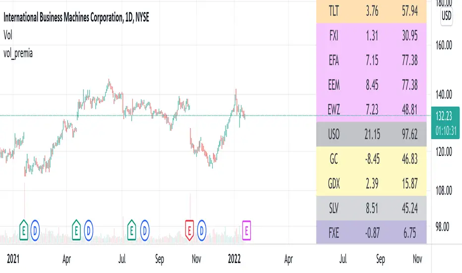
vol_premiaThis script shows the volatility risk premium for several instruments. The premium is simply "IV30 - RV20". Although Tradingview doesn't provide options prices, CBOE publishes 30-day implied volatilities for many instruments (most of which are VIX variations). CBOE calculates these in a standard way, weighting at- and out-of-the-money IVs for options that expire in 30 days, on average. For realized volatility, I used the standard deviation of log returns. Since there are twenty trading periods in 30 calendar days, IV30 can be compared to RV20. The "premium" is the difference, which reflects market participants' expectation for how much upcoming volatility will over- or under-shoot recent volatility.
The script loads pretty slow since there are lots of symbols, so feel free to delete the ones you don't care about. Hopefully the code is straightforward enough. I won't list the meaning of every symbols here, since I might change them later, but you can type them into tradingview for data, and read about their volatility index on CBOE's website. Some of the more well-known ones are:
ES: S&P futures, which I prefer to the SPX index). Its implied volatility is VIX.
USO: the oil ETF representing WTI future prices. Its IV is OVX.
GDX: the gold miner's ETF, which is usually more volatile than gold. Its IV is VXGDX.
FXI: a china ETF, whose volatility is VXFXI.
And so on. In addition to the premium, the "percentile" column shows where this premium ranks among the previous 252 trading days. 100 = the highest premium, 0 = the lowest premium.
IV/HV Ratio's [Nic]IV is implied volatility
HV is historic realized volatility
Seneca teaches that we often suffer more in our minds than in reality, and the same is true with the stock market. This indicator can help identify when people are over paying for implied volatility relative to real volatility . This means that short sellers are over paying for puts and can be squeezed into covering their positions, resulting in a massive rally.
The indicator can track this spread over many time frames, when the short time frame is much higher than the lower time frames, consider it a signal-of-interest.

SPY Expected Move by VIXThis indicator shows 1 and 2 standard deviation price move from the VWAP based on VIX. Implied Volatility (IV) is being used extensively in the Option world to project the Expected Move for the underlying instrument. VIX is used as a proxy for SPY's IV for 30 days.
This indicator is meaningful only for SPY but can be used in any other instrument which has a strong correlation to SPY.

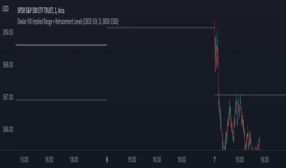
Dealar VIX Implied Range + Retracement LevelsThis Implied range Is derived by the VIX(1 sd annual +/- Implied move.)
This Indicator plots the daily Implied range, A lot of quantitative trading firms/ MM firms hedge their delta & gamma exposure around the Implied range(prop calc). I have added retracement levels as well, so you have more pivot levels.
Enjoy!
vol_rangesThis script shows three measures of volatility:
historical (hv): realized volatility of the recent past
median (mv): a long run average of realized volatility
implied (iv): a user-defined volatility
Historical and median volatility are based on the EWMA, rather than standard deviation, method of calculating volatility. Since Tradingview's built in ema function uses a window, the "window" parameter determines how much historical data is used to calculate these volatility measures. E.g. 30 on a daily chart means the previous 30 days.
The plots above and below historical candles show past projections based on these measures. The "periods to expiration" dictates how far the projection extends. At 30 periods to expiration (default), the plot will indicate the one standard deviation range from 30 periods ago. This is calculated by multiplying the volatility measure by the square root of time. For example, if the historical volatility (hv) was 20% and the window is 30, then the plot is drawn over: close * 1.2 * sqrt(30/252).
At the most recent candle, this same calculation is simply drawn as a line projecting into the future.
This script is intended to be used with a particular options contract in mind. For example, if the option expires in 15 days and has an implied volatility of 25%, choose 15 for the window and 25 for the implied volatility options. The ranges drawn will reflect the two standard deviation range both in the future (lines) and at any point in the past (plots) for HV (blue), MV (red), and IV (grey).

VIX-VXV-Ratio-Buschi
English:
This script shows the ratio between the VIX (implied volatility of SPX options over the next month) and the VXV (implied volatility of SPX options over the next three months). Since in normal "Contango" mode, the VXV should be higher than the VIX, the crossing under 1.0 or maybe 0.95 after a volatility spike could be a sign for a calming market or at least a calming volatility.
Deutsch:
Dieses Skript zeigt das Verhältnis zwischen dem VIX (implizite Volatilität der SPX-Optionen über den nächsten Monat) und dem VXV (implizite Volatilität der SPX-Optionen über die nächsten drei Monate). Da im normalen "Contango"-Modus der VXV höher als der VIX liegen sollte, kann das Abfallen unter 1,0 oder 0,95 nach einer Volatilitätsspitze ein Anzeichen für einen ruhiger werdenden Markt oder zumindest eine ruhiger werdende Volatilität sein.

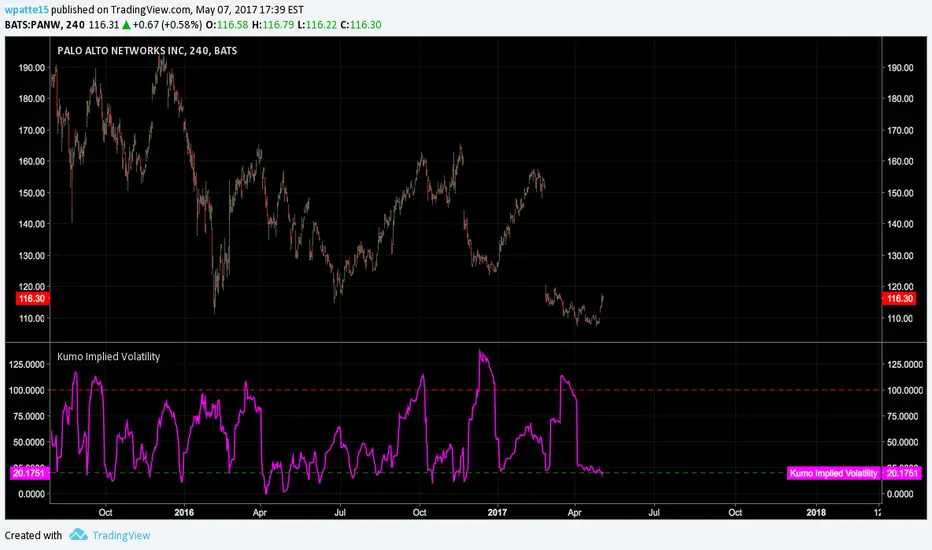
Kumo Implied VolatilityFrom ProRealCode www.prorealcode.com
"In my pursuit to quantify the Ichimoku indicator, I have tried to quantify implied volatility by measuring the Kumo thickness. Firstly, I took the absolute value of the distance between SpanA and SpanB, I then normalized the value and created standard deviation bands. Now I can compare the Kumo thickness with the average thickness over 200 periods. When the value goes above 100, it implies that the Kumo is thicker than 2 standard deviations of the average (there is therefore only a 5% chance that this happens). A reading over 100 might indicate trend exhaustion and a reading below 20 indicates low volatility and Kumo twists (I chose 20 only by observation and not statistical significance). Interestingly, this indicator sometime gives similar information to ADX. So far, the best use for this indicator is as a setup indicator for trend exhaustion or low volatility breakouts from Kumo twists. Extreme readings before Kumo breakouts looks interesting."
VIX Implied MovesKey Features:
Three Timeframe Bands:
Daily: Blue bands showing ±1σ expected move
Weekly: Green bands showing ±1σ expected move
30-Day: Red bands showing ±1σ expected move
Calculation Methodology:
Uses VIX's annualized volatility converted to specific timeframes using square root of time rule
Trading day convention (252 days/year)
Band width = Price × (VIX/100) ÷ √(number of periods)
Visual Features:
Colored semi-transparent backgrounds between bands
Progressive line thickness (thinner for shorter timeframes)
Real-time updates as VIX and ES prices change
Example Calculation (VIX=20, ES=5000):
Daily move = 5000 × (20/100)/√252 ≈ ±63 points
Weekly move = 5000 × (20/100)/√50 ≈ ±141 points
Monthly move = 5000 × (20/100)/√21 ≈ ±218 points
This indicator helps visualize expected price ranges based on current volatility conditions, with wider bands indicating higher market uncertainty. The probabilistic ranges represent 68% confidence levels (1 standard deviation) derived from options pricing.

Wavetrend in Dynamic Zones with Kumo Implied VolatilityI was asked to do one of those, so here we go...
As always free and open source as it should be. Do not pay for such indicators!
A WaveTrend Indicator or also widely known as "Market Cipher" is an Indicator that is based on Moving Averages, therefore its an "lagging indicator". Lagging indicators are best used in combination with leading indicators. In this script the "leading indicator" component are Daily, Weekly or Monthly Pivots . These Pivots can be used as dynamic Support and Resistance , Stoploss, Take Profit etc.
This indicator combination is best used in larger timeframes. For lower timeframes you might need to change settings to your liking.
The general Wavetrend settings are the same that are used in Market Cipher, Market Liberator and such popular indicators.
What are these circles?
-These are the WaveTrend Divergences. Red for Regular-Bearish. Orange for Hidden-Bearish. Green for Regular-Bullish. Aqua for Hidden-Bullish.
What are these white, orange and aqua triangles?
-These are the WaveTrend Pivots. A Pivot counter was added. Every time a pivot is lower than the previous one, an orange triangle is printed, every time a pivot is higher than the previous one an aqua triangle is printed. That mimics a very common way Wavetrend is being used for trading when using those other paid Wavetrend indicators.
What are these Orange and Aqua Zones?
-These are Dynamic Zones based on the indicator itself, they offer more information than static zones. Of course static lines are also included and can be adjusted.
What are the lines between the waves?
-This is a Kumo Cloud Implied Volatility indicator. It is color coded and can be used to indicate if a major market move/bottom/top happened.
What are those numbers on the right?
-The first number is a Bollinger Band indicator that shows if said Bollinger Band is in a state of Oversold/Overbought, the second number is the actual Bollinger Band Width that indicates if the Bollinger Band squeezes, normally that happens right before the market makes an explosive move.
Please keep in mind that this indicator is a tool and not a strategy, do not blindly trade signals, do your own research first! Use this indicator in conjunction with other indicators to get multiple confirmations.

OHLC Volatility Estimators by @Xel_arjonaDISCLAIMER:
The Following indicator/code IS NOT intended to be a formal investment advice or recommendation by the author, nor should be construed as such. Users will be fully responsible by their use regarding their own trading vehicles/assets.
The embedded code and ideas within this work are FREELY AND PUBLICLY available on the Web for NON LUCRATIVE ACTIVITIES and must remain as is by Creative-Commons as TradingView's regulations. Any use, copy or re-use of this code should mention it's origin as it's authorship.
WARNING NOTICE!
THE INCLUDED FUNCTION MUST BE CONSIDERED AS DEBUGING CODE The models included in the function have been taken from openly sources on the web so they could have some errors as in the calculation scheme and/or in it's programatic scheme. Debugging are welcome.
WHAT'S THIS?
Here's a full collection of candle based (compressed tick) Volatility Estimators given as a function, openly available for free, it can print IMPLIED VOLATILITY by an external symbol ticker like INDEX:VIX.
Models included in the volatility calculation function:
CLOSE TO CLOSE: This is the classic estimator by rule, sometimes referred as HISTORICAL VOLATILITY and is the must common, accepted and widely used out there. Is based on traditional Standard Deviation method derived from the logarithm return of current close from yesterday's.
ELASTIC WEIGHTED MOVING AVERAGE: This estimator has been used by RiskMetriks®. It's calculation is based on an ElasticWeightedMovingAverage Standard Deviation method derived from the logarithm return of current close from yesterday's. It can be viewed or named as an EXPONENTIAL HISTORICAL VOLATILITY model.
PARKINSON'S: The Parkinson number, or High Low Range Volatility, developed by the physicist, Michael Parkinson, in 1980 aims to estimate the Volatility of returns for a random walk using the high and low in any particular period. IVolatility.com calculates daily Parkinson values. Prices are observed on a fixed time interval. n=10, 20, 30, 60, 90, 120, 150, 180 days.
ROGERS-SATCHELL: The Rogers-Satchell function is a volatility estimator that outperforms other estimators when the underlying follows a Geometric Brownian Motion (GBM) with a drift (historical data mean returns different from zero). As a result, it provides a better volatility estimation when the underlying is trending. However, this Rogers-Satchell estimator does not account for jumps in price (Gaps). It assumes no opening jump. The function uses the open, close, high, and low price series in its calculation and it has only one parameter, which is the period to use to estimate the volatility.
YANG-ZHANG: Yang and Zhang were the first to derive an historical volatility estimator that has a minimum estimation error, is independent of the drift, and independent of opening gaps. This estimator is maximally 14 times more efficient than the close-to-close estimator.
LOGARITHMIC GARMAN-KLASS: The former is a pinescript transcript of the model defined as in iVolatility . The metric used is a combination of the overnight, high/low and open/close range. Such a volatility metric is a more efficient measure of the degree of volatility during a given day. This metric is always positive.
