DCA + Martingale strategy.DCA + Martingale: smart synergy for volatile markets
Tame market swings with a powerful hybrid strategy that marries the discipline of Dollar‑Cost Averaging (DCA) with the aggressive recovery logic of the Martingale system. This approach turns price dips into opportunities — systematically building positions while keeping risk in check.
How it works:
1. Entry trigger
The strategy activates when the asset price drops by a predefined percentage on the 1‑hour timeframe. This ensures you only engage when a meaningful pullback occurs, avoiding premature entries.
2. DCA grid for controlled averaging
Once the entry condition is met, a grid of buy orders is deployed:
Each subsequent order is placed at progressively lower price levels (e.g., every 2–5% drop).
Order sizes can be fixed or follow a progressive scale (e.g., 1x, 1.5x, 2x the initial amount).
This dilutes your average entry price, improving the breakeven point as the market corrects.
3. Martingale‑style recovery mechanism
After each unsuccessful trade (i.e., price continues falling), the next position size is increased — not necessarily doubled, but scaled according to your risk tolerance. This accelerates recovery potential when the trend reverses.
4. Take‑profit with a fixed percentage target
A simple, predefined profit target (e.g., +3–7%) is set for the entire averaged position. Once hit, all open trades close, locking in gains. This prevents over‑exposure during uncertain reversals.
Key advantages
Psychological edge: removes emotional decision‑making by automating entries and exits.
Cost optimization: lowers average entry during downtrends, improving profit potential.
Controlled aggression: Martingale logic helps recoup losses faster without infinite scaling.
Flexibility: parameters (entry %, grid spacing, position sizing, TP) are fully customizable.
Risk management essentials
Stop‑loss safeguard: a hard stop‑loss (e.g., 10–15% below the lowest grid level) prevents catastrophic drawdowns in prolonged downtrends.
Position sizing: never risk more than 1–3% of capital per grid cycle.
Market context: best suited for assets with mean‑reverting behavior and moderate volatility. Avoid strong, sustained trends.
Capital buffer: ensure sufficient reserves to withstand multiple grid levels without margin calls.
When to use it
During sideways or range‑bound markets with regular pullbacks.
On assets with historical tendency to recover from short‑term dips.
When you expect a bounce but can’t pinpoint the exact bottom.
Bottom line
DCA + Martingale isn’t a «set‑and‑forget» miracle — it’s a disciplined framework for turning volatility into opportunity. Combine it with rigorous risk rules, and you’ll navigate downtrends with precision, turning market noise into structured profit potential.
Sisihan Piawai

Cat Cushion Position SizingThis strategy is for people who don’t want to guess position size every time.
It looks at how volatile the market is and then tells you how many units to hold so your risk per trade stays roughly the same – whether the chart is calm or crazy.
What it does
Measures how “shaky” the price is day by day (volatility)
Blends recent volatility with a long-term average so it doesn’t overreact to one weird day
Uses your Risk per Trade (%) setting to calculate how big your position should be
Adds a buffer zone so it doesn’t trade every tiny wiggle and burn commissions
Shows a small performance table on the chart:
• Average annual return (from backtest)
• Sharpe ratio
• Average drawdown per trade
• Current position size as % of equity
How it thinks about risk
When the market is calmer → volatility is lower → position size can be bigger
When the market is wild → volatility is higher → position size becomes smaller
You control the “spiciness” with:
• Risk per Trade (%) – how much of your equity you’re willing to risk on each position
• Change Sensitivity (%) – wider buffer = fewer trades, lower costs; tighter buffer = more frequent rebalancing
Good use cases
Index ETFs (e.g. AMEX:SPY , NASDAQ:ACWI ) or other liquid instruments
People who:
• Already have a direction/idea (bullish on the index long term)
• Want the position sizing to adapt automatically with volatility
• Prefer “set the rules, let it run” rather than staring at the screen
Inputs to pay attention to
Risk per Trade (%)
• Conservative: ~1–2%
• Balanced: ~3–4%
• Aggressive: 5%+ (handle with care)
Important notes
This is a position sizing / risk strategy, not a magical “always win” tool
Works best when combined with:
• A clear idea of what you want to trade (e.g. broad index ETFs)
• A realistic risk profile (don’t just max the risk because the backtest looks better)
Backtest results are not a promise of future returns
Educational use only – this is not financial advice. Please test on your own, tweak to your comfort level, and don’t bet the rent money 😉
If you like systematic, “low-drama” investing (and want to spend more time chilling like a cat 🐱), this script helps the math side stay under control in the background.

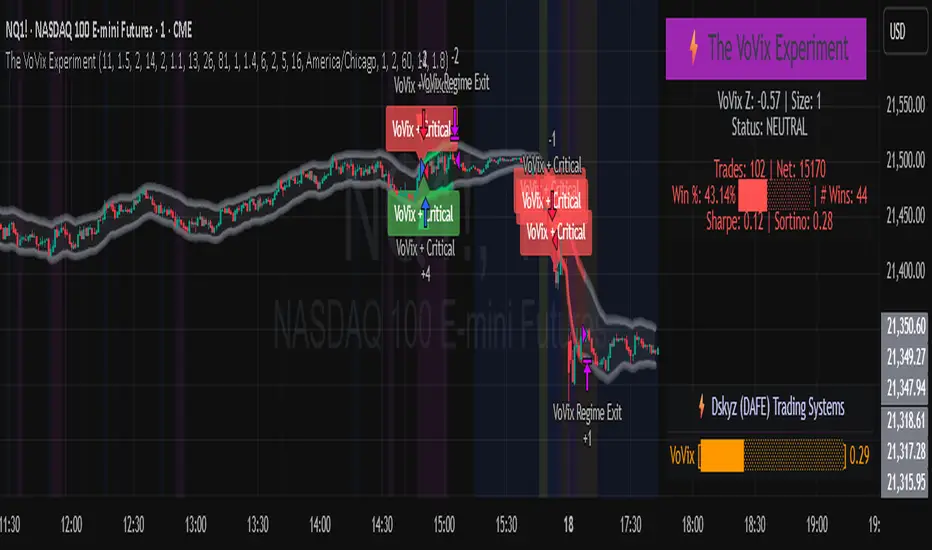
The VoVix Experiment The VoVix Experiment
The VoVix Experiment is a next-generation, regime-aware, volatility-adaptive trading strategy for futures, indices, and more. It combines a proprietary VoVix (volatility-of-volatility) anomaly detector with price structure clustering and critical point logic, only trading when multiple independent signals align. The system is designed for robustness, transparency, and real-world execution.
Logic:
VoVix Regime Engine: Detects pre-move volatility anomalies using a fast/slow ATR ratio, normalized by Z-score. Only trades when a true regime spike is detected, not just random volatility.
Cluster & Critical Point Filters: Price structure and volatility clustering must confirm the VoVix signal, reducing false positives and whipsaws.
Adaptive Sizing: Position size scales up for “super-spikes” and down for normal events, always within user-defined min/max.
Session Control: Trades only during user-defined hours and days, avoiding illiquid or high-risk periods.
Visuals: Aurora Flux Bands (From another Original of Mine (Options Flux Flow): glow and change color on signals, with a live dashboard, regime heatmap, and VoVix progression bar for instant insight.
Backtest Settings
Initial capital: $10,000
Commission: Conservative, realistic roundtrip cost:
15–20 per contract (including slippage per side) I set this to $25
Slippage: 3 ticks per trade
Symbol: CME_MINI:NQ1!
Timeframe: 15 min (but works on all timeframes)
Order size: Adaptive, 1–2 contracts
Session: 5:00–15:00 America/Chicago (default, fully adjustable)
Why these settings?
These settings are intentionally strict and realistic, reflecting the true costs and risks of live trading. The 10,000 account size is accessible for most retail traders. 25/contract including 3 ticks of slippage are on the high side for MNQ, ensuring the strategy is not curve-fit to perfect fills. If it works here, it will work in real conditions.
Forward Testing: (This is no guarantee. I've provided these results to show that executions perform as intended. Test were done on Tradovate)
ALL TRADES
Gross P/L: $12,907.50
# of Trades: 64
# of Contracts: 186
Avg. Trade Time: 1h 55min 52sec
Longest Trade Time: 55h 46min 53sec
% Profitable Trades: 59.38%
Expectancy: $201.68
Trade Fees & Comm.: $(330.95)
Total P/L: $12,576.55
Winning Trades: 59.38%
Breakeven Trades: 3.12%
Losing Trades: 37.50%
Link: www.dropbox.com
Inputs & Tooltips
VoVix Regime Execution: Enable/disable the core VoVix anomaly detector.
Volatility Clustering: Require price/volatility clusters to confirm VoVix signals.
Critical Point Detector: Require price to be at a statistically significant distance from the mean (regime break).
VoVix Fast ATR Length: Short ATR for fast volatility detection (lower = more sensitive).
VoVix Slow ATR Length: Long ATR for baseline regime (higher = more stable).
VoVix Z-Score Window: Lookback for Z-score normalization (higher = smoother, lower = more reactive).
VoVix Entry Z-Score: Minimum Z-score for a VoVix spike to trigger a trade.
VoVix Exit Z-Score: Z-score below which the regime is considered decayed (exit).
VoVix Local Max Window: Bars to check for local maximum in VoVix (higher = stricter).
VoVix Super-Spike Z-Score: Z-score for “super” regime events (scales up position size).
Min/Max Contracts: Adaptive position sizing range.
Session Start/End Hour: Only trade between these hours (exchange time).
Allow Weekend Trading: Enable/disable trading on weekends.
Session Timezone: Timezone for session filter (e.g., America/Chicago for CME).
Show Trade Labels: Show/hide entry/exit labels on chart.
Flux Glow Opacity: Opacity of Aurora Flux Bands (0–100).
Flux Band EMA Length: EMA period for band center.
Flux Band ATR Multiplier: Width of bands (higher = wider).
Compliance & Transparency
* No hidden logic, no repainting, no pyramiding.
* All signals, sizing, and exits are fully explained and visible.
* Backtest settings are stricter than most real accounts.
* All visuals are directly tied to the strategy logic.
* This is not a mashup or cosmetic overlay; every component is original and justified.
Disclaimer
Trading is risky. This script is for educational and research purposes only. Do not trade with money you cannot afford to lose. Past performance is not indicative of future results. Always test in simulation before live trading.
Proprietary Logic & Originality Statement
This script, “The VoVix Experiment,” is the result of original research and development. All core logic, algorithms, and visualizations—including the VoVix regime detection engine, adaptive execution, volatility/divergence bands, and dashboard—are proprietary and unique to this project.
1. VoVix Regime Logic
The concept of “volatility of volatility” (VoVix) is an original quant idea, not a standard indicator. The implementation here (fast/slow ATR ratio, Z-score normalization, local max logic, super-spike scaling) is custom and not found in public TradingView scripts.
2. Cluster & Critical Point Logic
Volatility clustering and “critical point” detection (using price distance from a rolling mean and standard deviation) are general quant concepts, but the way they are combined and filtered here is unique to this script. The specific logic for “clustered chop” and “critical point” is not a copy of any public indicator.
3. Adaptive Sizing
The adaptive sizing logic (scaling contracts based on regime strength) is custom and not a standard TradingView feature or public script.
4. Time Block/Session Control
The session filter is a common feature in many strategies, but the implementation here (with timezone and weekend control) is written from scratch.
5. Aurora Flux Bands (From another Original of Mine (Options Flux Flow)
The “glowing” bands are inspired by the idea of volatility bands (like Bollinger Bands or Keltner Channels), but the visual effect, color logic, and integration with regime signals are original to this script.
6. Dashboard, Watermark, and Metrics
The dashboard, real-time Sharpe/Sortino, and VoVix progression bar are all custom code, not copied from any public script.
What is “standard” or “common quant practice”?
Using ATR, EMA, and Z-score are standard quant tools, but the way they are combined, filtered, and visualized here is unique. The structure and logic of this script are original and not a mashup of public code.
This script is 100% original work. All logic, visuals, and execution are custom-coded for this project. No code or logic is directly copied from any public or private script.
Use with discipline. Trade your edge.
— Dskyz, for DAFE Trading Systems
REVELATIONS (VoVix - PoC) REVELATIONS (VoVix - POC): True Regime Detection Before the Move
Let’s not sugarcoat it: Most strategies on TradingView are recycled—RSI, MACD, OBV, CCI, Stochastics. They all lag. No matter how many overlays you stack, every one of these “standard” indicators fires after the move is underway. The retail crowd almost always gets in late. That’s never been enough for my team, for DAFE, or for anyone who’s traded enough to know the real edge vanishes by the time the masses react.
How is this different?
REVELATIONS (VoVix - POC) was engineered from raw principle, structured to detect pre-move regime change—before standard technicals even light up. We built, tested, and refined VoVix to answer one hard question:
What if you could see the spike before the trend?
Here’s what sets this system apart, line-by-line:
o True volatility-of-volatility mathematics: It’s not just "ATR of ATR" or noise smoothing. VoVix uses normalized, multi-timeframe v-vol spikes, instantly detecting orderbook stress and "outlier" market events—before the chart shows them as trends.
o Purist regime clustering: Every trade is enabled only during coordinated, multi-filter regime stress. No more signals in meaningless chop.
o Nonlinear entry logic: No trade is ever sent just for a “good enough” condition. Every entry fires only if every requirement is aligned—local extremes, super-spike threshold, regime index, higher timeframe, all must trigger in sync.
o Adaptive position size: Your contracts scale up with event strength. Tiny size during nominal moves, max leverage during true regime breaks—never guesswork, never static exposure.
o All exits governed by regime decay logic: Trades are closed not just on price targets but at the precise moment the market regime exhausts—the hardest part of systemic trading, now solved.
How this destroys the lag:
Standard indicators (RSI, MACD, OBV, CCI, and even most “momentum” overlays) simply tell you what already happened. VoVix triggers as price structure transitions—anyone running these generic scripts will trade behind the move while VoVix gets in as stress emerges. Real alpha comes from anticipation, not confirmation.
The visuals only show what matters:
Top right, you get a live, live quant dashboard—regime index, current position size, real-time performance (Sharpe, Sortino, win rate, and wins). Bottom right: a VoVix "engine bar" that adapts live with regime stress. Everything you see is a direct function of logic driving this edge—no cosmetics, no fake momentum.
Inputs/Signals—explained carefully for clarity:
o ATR Fast Length & ATR Slow Length:
These are the heart of VoVix’s regime sensing. Fast ATR reacts to sharp volatility; Slow ATR is stability baseline. Lower Fast = reacts to every twitch; higher Slow = requires more persistent, “real” regime shifts.
Tip: If you want more signals or faster markets, lower ATR Fast. To eliminate noise, raise ATR Slow.
o ATR StdDev Window: Smoothing for volatility-of-volatility normalization. Lower = more jumpy, higher = only the cleanest spikes trigger.
Tip: Shorten for “jumpy” assets, raise for indices/futures.
o Base Spike Threshold: Think of this as your “minimum event strength.” If the current move isn’t volatile enough (normalized), no signal.
Tip: Higher = only biggest moves matter. Lower for more signals but more potential noise.
o Super Spike Multiplier: The “are you sure?” test—entry only when the current spike is this multiple above local average.
Tip: Raise for ultra-selective/swing-trading; lower for more active style.
Regime & MultiTF:
o Regime Window (Bars):
How many bars to scan for regime cluster “events.” Short for turbo markets, long for big swings/trends only.
o Regime Event Count: Only trade when this many spikes occur within the Regime Window—filters for real stress, not isolated ticks.
Tip: Raise to only ever trade during true breakouts/crashes.
o Local Window for Extremes:
How many bars to check that a spike is a local max.
Tip: Raise to demand only true, “clearest” local regime events; lower for early triggers.
o HTF Confirm:
Higher timeframe regime confirmation (like 45m on an intraday chart). Ensures any event you act on is visible in the broader context.
Tip: Use higher timeframes for only major moves; lower for scalping or fast regimes.
Adaptive Sizing:
o Max Contracts (Adaptive): The largest size your system will ever scale to, even on extreme event.
Tip: Lower for small accounts/conservative risk; raise on big accounts or when you're willing to go big only on outlier events.
o Min Contracts (Adaptive): The “toe-in-the-water.” Smallest possible trade.
Tip: Set as low as your broker/exchange allows for safety, or higher if you want to always have meaningful skin in the game.
Trade Management:
o Stop %: Tightness of your stop-loss relative to entry. Lower for tighter/safer, higher for more breathing room at cost of greater drawdown.
o Take Profit %: How much you'll hold out for on a win. Lower = more scalps. Higher = only run with the best.
o Decay Exit Sensitivity Buffer: Regime index must dip this far below the trading threshold before you exit for “regime decay.”
Tip: 0 = exit as soon as stress fails, higher = exits only on stronger confirmation regime is over.
o Bars Decay Must Persist to Exit: How long must decay be present before system closes—set higher to avoid quick fades and whipsaws.
Backtest Settings
Initial capital: $10,000
Commission: Conservative, realistic roundtrip cost:
15–20 per contract (including slippage per side) I set this to $25
Slippage: 3 ticks per trade
Symbol: CME_MINI:NQ1!
Timeframe: 1 min (but works on all timeframes)
Order size: Adaptive, 1–3 contracts
No pyramiding, no hidden DCA
Why these settings?
These settings are intentionally strict and realistic, reflecting the true costs and risks of live trading. The 10,000 account size is accessible for most retail traders. 25/contract including 3 ticks of slippage are on the high side for NQ, ensuring the strategy is not curve-fit to perfect fills. If it works here, it will work in real conditions.
Tip: Set to 1 for instant regime exit; raise for extra confirmation (less whipsaw risk, exits held longer).
________________________________________
Bottom line: Tune the sensitivity, selectivity, and risk of REVELATIONS by these inputs. Raise thresholds and windows for only the best, most powerful signals (institutional style); lower for activity (scalpers, fast cryptos, signals in constant motion). Sizing is always adaptive—never static or martingale. Exits are always based on both price and regime health. Every input is there for your control, not to sell “complexity.” Use with discipline, and make it your own.
This strategy is not just a technical achievement: It’s a statement about trading smarter, not just more.
* I went back through the code to make sure no the strategy would not suffer from repainting, forward looking, or any frowned upon loopholes.
Disclaimer:
Trading is risky and carries the risk of substantial loss. Do not use funds you aren’t prepared to lose. This is for research and informational purposes only, not financial advice. Backtest, paper trade, and know your risk before going live. Past performance is not a guarantee of future results.
Expect more: We’ll keep pushing the standard, keep evolving the bar until “quant” actually means something in the public code space.
Use with clarity, use with discipline, and always trade your edge.
— Dskyz , for DAFE Trading Systems

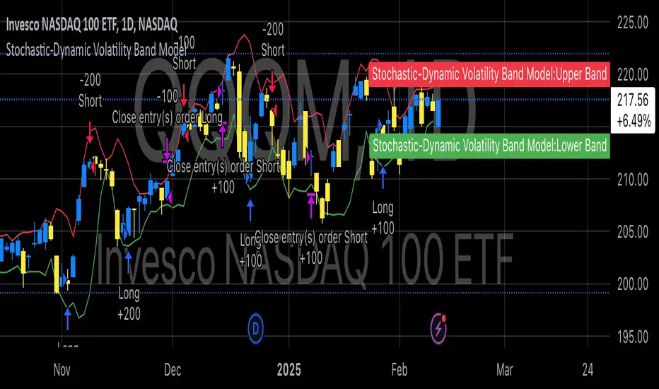
Stochastic-Dynamic Volatility Band ModelThe Stochastic-Dynamic Volatility Band Model is a quantitative trading approach that leverages statistical principles to model market volatility and generate buy and sell signals. The strategy is grounded in the concepts of volatility estimation and dynamic market regimes, where the core idea is to capture price fluctuations through stochastic models and trade around volatility bands.
Volatility Estimation and Band Construction
The volatility bands are constructed using a combination of historical price data and statistical measures, primarily the standard deviation (σ) of price returns, which quantifies the degree of variation in price movements over a specific period. This methodology is based on the classical works of Black-Scholes (1973), which laid the foundation for using volatility as a core component in financial models. Volatility is a crucial determinant of asset pricing and risk, and it plays a pivotal role in this strategy's design.
Entry and Exit Conditions
The entry conditions are based on the price’s relationship with the volatility bands. A long entry is triggered when the price crosses above the lower volatility band, indicating that the market may have been oversold or is experiencing a reversal to the upside. Conversely, a short entry is triggered when the price crosses below the upper volatility band, suggesting overbought conditions or a potential market downturn.
These entry signals are consistent with the mean reversion theory, which asserts that asset prices tend to revert to their long-term average after deviating from it. According to Poterba and Summers (1988), mean reversion occurs due to overreaction to news or temporary disturbances, leading to price corrections.
The exit condition is based on the number of bars that have elapsed since the entry signal. Specifically, positions are closed after a predefined number of bars, typically set to seven bars, reflecting a short-term trading horizon. This exit mechanism is in line with short-term momentum trading strategies discussed in literature, where traders capitalize on price movements within specific timeframes (Jegadeesh & Titman, 1993).
Market Adaptability
One of the key features of this strategy is its dynamic nature, as it adapts to the changing volatility environment. The volatility bands automatically adjust to market conditions, expanding in periods of high volatility and contracting when volatility decreases. This dynamic adjustment helps the strategy remain robust across different market regimes, as it is capable of identifying both trend-following and mean-reverting opportunities.
This dynamic adaptability is supported by the adaptive market hypothesis (Lo, 2004), which posits that market participants evolve their strategies in response to changing market conditions, akin to the adaptive nature of biological systems.
References:
Black, F., & Scholes, M. (1973). The Pricing of Options and Corporate Liabilities. Journal of Political Economy, 81(3), 637-654.
Bollinger, J. (1980). Bollinger on Bollinger Bands. Wiley.
Jegadeesh, N., & Titman, S. (1993). Returns to Buying Winners and Selling Losers: Implications for Stock Market Efficiency. Journal of Finance, 48(1), 65-91.
Lo, A. W. (2004). The Adaptive Markets Hypothesis: Market Efficiency from an Evolutionary Perspective. Journal of Portfolio Management, 30(5), 15-29.
Poterba, J. M., & Summers, L. H. (1988). Mean Reversion in Stock Prices: Evidence and Implications. Journal of Financial Economics, 22(1), 27-59.
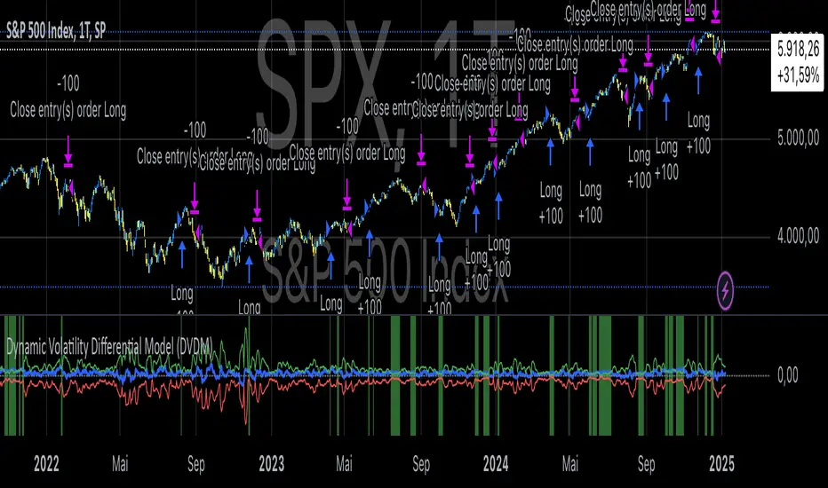
Dynamic Volatility Differential Model (DVDM)The Dynamic Volatility Differential Model (DVDM) is a quantitative trading strategy designed to exploit the spread between implied volatility (IV) and historical (realized) volatility (HV). This strategy identifies trading opportunities by dynamically adjusting thresholds based on the standard deviation of the volatility spread. The DVDM is versatile and applicable across various markets, including equity indices, commodities, and derivatives such as the FDAX (DAX Futures).
Key Components of the DVDM:
1. Implied Volatility (IV):
The IV is derived from options markets and reflects the market’s expectation of future price volatility. For instance, the strategy uses volatility indices such as the VIX (S&P 500), VXN (Nasdaq 100), or RVX (Russell 2000), depending on the target market. These indices serve as proxies for market sentiment and risk perception (Whaley, 2000).
2. Historical Volatility (HV):
The HV is computed from the log returns of the underlying asset’s price. It represents the actual volatility observed in the market over a defined lookback period, adjusted to annualized levels using a multiplier of \sqrt{252} for daily data (Hull, 2012).
3. Volatility Spread:
The difference between IV and HV forms the volatility spread, which is a measure of divergence between market expectations and actual market behavior.
4. Dynamic Thresholds:
Unlike static thresholds, the DVDM employs dynamic thresholds derived from the standard deviation of the volatility spread. The thresholds are scaled by a user-defined multiplier, ensuring adaptability to market conditions and volatility regimes (Christoffersen & Jacobs, 2004).
Trading Logic:
1. Long Entry:
A long position is initiated when the volatility spread exceeds the upper dynamic threshold, signaling that implied volatility is significantly higher than realized volatility. This condition suggests potential mean reversion, as markets may correct inflated risk premiums.
2. Short Entry:
A short position is initiated when the volatility spread falls below the lower dynamic threshold, indicating that implied volatility is significantly undervalued relative to realized volatility. This signals the possibility of increased market uncertainty.
3. Exit Conditions:
Positions are closed when the volatility spread crosses the zero line, signifying a normalization of the divergence.
Advantages of the DVDM:
1. Adaptability:
Dynamic thresholds allow the strategy to adjust to changing market conditions, making it suitable for both low-volatility and high-volatility environments.
2. Quantitative Precision:
The use of standard deviation-based thresholds enhances statistical reliability and reduces subjectivity in decision-making.
3. Market Versatility:
The strategy’s reliance on volatility metrics makes it universally applicable across asset classes and markets, ensuring robust performance.
Scientific Relevance:
The strategy builds on empirical research into the predictive power of implied volatility over realized volatility (Poon & Granger, 2003). By leveraging the divergence between these measures, the DVDM aligns with findings that IV often overestimates future volatility, creating opportunities for mean-reversion trades. Furthermore, the inclusion of dynamic thresholds aligns with risk management best practices by adapting to volatility clustering, a well-documented phenomenon in financial markets (Engle, 1982).
References:
1. Christoffersen, P., & Jacobs, K. (2004). The importance of the volatility risk premium for volatility forecasting. Journal of Financial and Quantitative Analysis, 39(2), 375-397.
2. Engle, R. F. (1982). Autoregressive conditional heteroskedasticity with estimates of the variance of United Kingdom inflation. Econometrica, 50(4), 987-1007.
3. Hull, J. C. (2012). Options, Futures, and Other Derivatives. Pearson Education.
4. Poon, S. H., & Granger, C. W. J. (2003). Forecasting volatility in financial markets: A review. Journal of Economic Literature, 41(2), 478-539.
5. Whaley, R. E. (2000). The investor fear gauge. Journal of Portfolio Management, 26(3), 12-17.
This strategy leverages quantitative techniques and statistical rigor to provide a systematic approach to volatility trading, making it a valuable tool for professional traders and quantitative analysts.
BTCUSD Momentum After Abnormal DaysThis indicator identifies abnormal days in the Bitcoin market (BTCUSD) based on daily returns exceeding specific thresholds defined by a statistical approach. It is inspired by the findings of Caporale and Plastun (2020), who analyzed the cryptocurrency market's inefficiencies and identified exploitable patterns, particularly around abnormal returns.
Key Concept:
Abnormal Days:
Days where the daily return significantly deviates (positively or negatively) from the historical average.
Positive abnormal days: Returns exceed the mean return plus k times the standard deviation.
Negative abnormal days: Returns fall below the mean return minus k times the standard deviation.
Momentum Effect:
As described in the academic paper, on abnormal days, prices tend to move in the direction of the abnormal return until the end of the trading day, creating momentum effects. This can be leveraged by traders for profit opportunities.
How It Works:
Calculation:
The script calculates the daily return as the percentage difference between the open and close prices. It then derives the mean and standard deviation of returns over a configurable lookback period.
Thresholds:
The script dynamically computes upper and lower thresholds for abnormal days using the mean and standard deviation. Days exceeding these thresholds are flagged as abnormal.
Visualization:
The mean return and thresholds are plotted as dynamic lines.
Abnormal days are visually highlighted with transparent green (positive) or red (negative) backgrounds on the chart.
References:
This indicator is based on the methodology discussed in "Momentum Effects in the Cryptocurrency Market After One-Day Abnormal Returns" by Caporale and Plastun (2020). Their research demonstrates that hourly returns during abnormal days exhibit a strong momentum effect, moving in the same direction as the abnormal return. This behavior contradicts the efficient market hypothesis and suggests profitable trading opportunities.
"Prices tend to move in the direction of abnormal returns till the end of the day, which implies the existence of a momentum effect on that day giving rise to exploitable profit opportunities" (Caporale & Plastun, 2020).

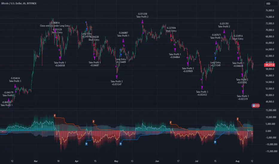
Multi-Step FlexiSuperTrend - Strategy [presentTrading]At the heart of this endeavor is a passion for continuous improvement in the art of trading
█ Introduction and How it is Different
The "Multi-Step FlexiSuperTrend - Strategy " is an advanced trading strategy that integrates the well-known SuperTrend indicator with a nuanced and dynamic approach to market trend analysis. Unlike conventional SuperTrend strategies that rely on static thresholds and fixed parameters, this strategy introduces multi-step take profit mechanisms that allow traders to capitalize on varying market conditions in a more controlled and systematic manner.
What sets this strategy apart is its ability to dynamically adjust to market volatility through the use of an incremental factor applied to the SuperTrend calculation. This adjustment ensures that the strategy remains responsive to both minor and major market shifts, providing a more accurate signal for entries and exits. Additionally, the integration of multi-step take profit levels offers traders the flexibility to scale out of positions, locking in profits progressively as the market moves in their favor.
BTC 6hr Long/Short Performance
█ Strategy, How it Works: Detailed Explanation
The Multi-Step FlexiSuperTrend strategy operates on the foundation of the SuperTrend indicator, but with several enhancements that make it more adaptable to varying market conditions. The key components of this strategy include the SuperTrend Polyfactor Oscillator, a dynamic normalization process, and multi-step take profit levels.
🔶 SuperTrend Polyfactor Oscillator
The SuperTrend Polyfactor Oscillator is the heart of this strategy. It is calculated by applying a series of SuperTrend calculations with varying factors, starting from a defined "Starting Factor" and incrementing by a specified "Increment Factor." The indicator length and the chosen price source (e.g., HLC3, HL2) are inputs to the oscillator.
The SuperTrend formula typically calculates an upper and lower band based on the average true range (ATR) and a multiplier (the factor). These bands determine the trend direction. In the FlexiSuperTrend strategy, the oscillator is enhanced by iteratively applying the SuperTrend calculation across different factors. The iterative process allows the strategy to capture both minor and significant trend changes.
For each iteration (indexed by `i`), the following calculations are performed:
1. ATR Calculation: The Average True Range (ATR) is calculated over the specified `indicatorLength`:
ATR_i = ATR(indicatorLength)
2. Upper and Lower Bands Calculation: The upper and lower bands are calculated using the ATR and the current factor:
Upper Band_i = hl2 + (ATR_i * Factor_i)
Lower Band_i = hl2 - (ATR_i * Factor_i)
Here, `Factor_i` starts from `startingFactor` and is incremented by `incrementFactor` in each iteration.
3. Trend Determination: The trend is determined by comparing the indicator source with the upper and lower bands:
Trend_i = 1 (uptrend) if IndicatorSource > Upper Band_i
Trend_i = 0 (downtrend) if IndicatorSource < Lower Band_i
Otherwise, the trend remains unchanged from the previous value.
4. Output Calculation: The output of each iteration is determined based on the trend:
Output_i = Lower Band_i if Trend_i = 1
Output_i = Upper Band_i if Trend_i = 0
This process is repeated for each iteration (from 0 to 19), creating a series of outputs that reflect different levels of trend sensitivity.
Local
🔶 Normalization Process
To make the oscillator values comparable across different market conditions, the deviations between the indicator source and the SuperTrend outputs are normalized. The normalization method can be one of the following:
1. Max-Min Normalization: The deviations are normalized based on the range of the deviations:
Normalized Value_i = (Deviation_i - Min Deviation) / (Max Deviation - Min Deviation)
2. Absolute Sum Normalization: The deviations are normalized based on the sum of absolute deviations:
Normalized Value_i = Deviation_i / Sum of Absolute Deviations
This normalization ensures that the oscillator values are within a consistent range, facilitating more reliable trend analysis.
For more details:
🔶 Multi-Step Take Profit Mechanism
One of the unique features of this strategy is the multi-step take profit mechanism. This allows traders to lock in profits at multiple levels as the market moves in their favor. The strategy uses three take profit levels, each defined as a percentage increase (for long trades) or decrease (for short trades) from the entry price.
1. First Take Profit Level: Calculated as a percentage increase/decrease from the entry price:
TP_Level1 = Entry Price * (1 + tp_level1 / 100) for long trades
TP_Level1 = Entry Price * (1 - tp_level1 / 100) for short trades
The strategy exits a portion of the position (defined by `tp_percent1`) when this level is reached.
2. Second Take Profit Level: Similar to the first level, but with a higher percentage:
TP_Level2 = Entry Price * (1 + tp_level2 / 100) for long trades
TP_Level2 = Entry Price * (1 - tp_level2 / 100) for short trades
The strategy exits another portion of the position (`tp_percent2`) at this level.
3. Third Take Profit Level: The final take profit level:
TP_Level3 = Entry Price * (1 + tp_level3 / 100) for long trades
TP_Level3 = Entry Price * (1 - tp_level3 / 100) for short trades
The remaining portion of the position (`tp_percent3`) is exited at this level.
This multi-step approach provides a balance between securing profits and allowing the remaining position to benefit from continued favorable market movement.
█ Trade Direction
The strategy allows traders to specify the trade direction through the `tradeDirection` input. The options are:
1. Both: The strategy will take both long and short positions based on the entry signals.
2. Long: The strategy will only take long positions.
3. Short: The strategy will only take short positions.
This flexibility enables traders to tailor the strategy to their market outlook or current trend analysis.
█ Usage
To use the Multi-Step FlexiSuperTrend strategy, traders need to set the input parameters according to their trading style and market conditions. The strategy is designed for versatility, allowing for various market environments, including trending and ranging markets.
Traders can also adjust the multi-step take profit levels and percentages to match their risk management and profit-taking preferences. For example, in highly volatile markets, traders might set wider take profit levels with smaller percentages at each level to capture larger price movements.
The normalization method and the incremental factor can be fine-tuned to adjust the sensitivity of the SuperTrend Polyfactor Oscillator, making the strategy more responsive to minor market shifts or more focused on significant trends.
█ Default Settings
The default settings of the strategy are carefully chosen to provide a balanced approach between risk management and profit potential. Here is a breakdown of the default settings and their effects on performance:
1. Indicator Length (10): This parameter controls the lookback period for the ATR calculation. A shorter length makes the strategy more sensitive to recent price movements, potentially generating more signals. A longer length smooths out the ATR, reducing sensitivity but filtering out noise.
2. Starting Factor (0.618): This is the initial multiplier used in the SuperTrend calculation. A lower starting factor makes the SuperTrend bands closer to the price, generating more frequent trend changes. A higher starting factor places the bands further away, filtering out minor fluctuations.
3. Increment Factor (0.382): This parameter controls how much the factor increases with each iteration of the SuperTrend calculation. A smaller increment factor results in more gradual changes in sensitivity, while a larger increment factor creates a wider range of sensitivity across the iterations.
4. Normalization Method (None): The default is no normalization, meaning the raw deviations are used. Normalization methods like Max-Min or Absolute Sum can make the deviations more consistent across different market conditions, improving the reliability of the oscillator.
5. Take Profit Levels (2%, 8%, 18%): These levels define the thresholds for exiting portions of the position. Lower levels (e.g., 2%) capture smaller profits quickly, while higher levels (e.g., 18%) allow positions to run longer for more significant gains.
6. Take Profit Percentages (30%, 20%, 15%): These percentages determine how much of the position is exited at each take profit level. A higher percentage at the first level locks in more profit early, reducing exposure to market reversals. Lower percentages at higher levels allow for a portion of the position to benefit from extended trends.
HilalimSB Strategy HilalimSB A Wedding Gift 🌙
What is HilalimSB🌙?
First of all, as mentioned in the title, HilalimSB is a wedding gift.
HilalimSB - Revealing the Secrets of the Trend
HilalimSB is a powerful indicator designed to help investors analyze market trends and optimize trading strategies. Designed to uncover the secrets at the heart of the trend, HilalimSB stands out with its unique features and impressive algorithm.
Hilalim Algorithm and Fixed ATR Value:
HilalimSB is equipped with a special algorithm called "Hilalim" to detect market trends. This algorithm can delve into the depths of price movements to determine the direction of the trend and provide users with the ability to predict future price movements. Additionally, HilalimSB uses its own fixed Average True Range (ATR) value. ATR is an indicator that measures price movement volatility and is often used to determine the strength of a trend. The fixed ATR value of HilalimSB has been tested over long periods and its reliability has been proven. This allows users to interpret the signals provided by the indicator more reliably.
ATR Calculation Steps
1.True Range Calculation:
+ The True Range (TR) is the greatest of the following three values:
1. Current high minus current low
2. Current high minus previous close (absolute value)
3. Current low minus previous close (absolute value)
2.Average True Range (ATR) Calculation:
-The initial ATR value is calculated as the average of the TR values over a specified period
(typically 14 periods).
-For subsequent periods, the ATR is calculated using the following formula:
ATRt=(ATRt−1×(n−1)+TRt)/n
Where:
+ ATRt is the ATR for the current period,
+ ATRt−1 is the ATR for the previous period,
+ TRt is the True Range for the current period,
+ n is the number of periods.
Pine Script to Calculate ATR with User-Defined Length and Multiplier
Here is the Pine Script code for calculating the ATR with user-defined X length and Y multiplier:
//@version=5
indicator("Custom ATR", overlay=false)
// User-defined inputs
X = input.int(14, minval=1, title="ATR Period (X)")
Y = input.float(1.0, title="ATR Multiplier (Y)")
// True Range calculation
TR1 = high - low
TR2 = math.abs(high - close )
TR3 = math.abs(low - close )
TR = math.max(TR1, math.max(TR2, TR3))
// ATR calculation
ATR = ta.rma(TR, X)
// Apply multiplier
customATR = ATR * Y
// Plot the ATR value
plot(customATR, title="Custom ATR", color=color.blue, linewidth=2)
This code can be added as a new Pine Script indicator in TradingView, allowing users to calculate and display the ATR on the chart according to their specified parameters.
HilalimSB's Distinction from Other ATR Indicators
HilalimSB emerges with its unique Average True Range (ATR) value, presenting itself to users. Equipped with a proprietary ATR algorithm, this indicator is released in a non-editable form for users. After meticulous testing across various instruments with predetermined period and multiplier values, it is made available for use.
ATR is acknowledged as a critical calculation tool in the financial sector. The ATR calculation process of HilalimSB is conducted as a result of various research efforts and concrete data-based computations. Therefore, the HilalimSB indicator is published with its proprietary ATR values, unavailable for modification.
The ATR period and multiplier values provided by HilalimSB constitute the fundamental logic of a trading strategy. This unique feature aids investors in making informed decisions.
Visual Aesthetics and Clear Charts:
HilalimSB provides a user-friendly interface with clear and impressive graphics. Trend changes are highlighted with vibrant colors and are visually easy to understand. You can choose colors based on eye comfort, allowing you to personalize your trading screen for a more enjoyable experience. While offering a flexible approach tailored to users' needs, HilalimSB also promises an aesthetic and professional experience.
Strong Signals and Buy/Sell Indicators:
After completing test operations, HilalimSB produces data at various time intervals. However, we would like to emphasize to users that based on our studies, it provides the best signals in 1-hour chart data. HilalimSB produces strong signals to identify trend reversals. Buy or sell points are clearly indicated, allowing users to develop and implement trading strategies based on these signals.
For example, let's imagine you wanted to open a position on BTC on 2023.11.02. You are aware that you need to calculate which of the buying or selling transactions would be more profitable. You need support from various indicators to open a position. Based on the analysis and calculations it has made from the data it contains, HilalimSB would have detected that the graph is more suitable for a selling position, and by producing a sell signal at the most ideal selling point at 08:00 on 2023.11.02 (UTC+3 Istanbul), it would have informed you of the direction the graph would follow, allowing you to benefit positively from a 2.56% decline.
Technology and Innovation:
HilalimSB aims to enhance the trading experience using the latest technology. With its innovative approach, it enables users to discover market opportunities and support their decisions. Thus, investors can make more informed and successful trades. Real-Time Data Analysis: HilalimSB analyzes market data in real-time and identifies updated trends instantly. This allows users to make more informed trading decisions by staying informed of the latest market developments. Continuous Update and Improvement: HilalimSB is constantly updated and improved. New features are added and existing ones are enhanced based on user feedback and market changes. Thus, HilalimSB always aims to provide the latest technology and the best user experience.
Social Order and Intrinsic Motivation:
Negative trends such as widespread illegal gambling and uncontrolled risk-taking can have adverse financial effects on society. The primary goal of HilalimSB is to counteract these negative trends by guiding and encouraging users with data-driven analysis and calculable investment systems. This allows investors to trade more consciously and safely.
What is HilalimSB Strategy🌙?
HilalimSB Strategy is a strategy that is supported by the HilalimSB algorithm created by the creator of HilalimSB and continues transactions with take profit and stop loss levels determined by users who strategically and automatically open transactions as a result of the data it receives and automatically closes transactions under necessary conditions. It is a first in the tradingview world with its unique take profit and stop loss markings. HilalimSB Strategy is open to users' initiatives and is a trading strategy developed on BTC.
What does the HilalimSB Strategy target?
The main purpose of HilalimSB Strategy is to reduce the transaction load of traders and to be integrated into various brokerage firms and operated by automatic trading bots, and it is aimed to serve this purpose. In addition to the strategies currently available in the markets, HilalimSB Strategy offers a useful infrastructure to traders with its useful interface. HilalimSB Strategy, which was decided to be published as a result of various calculations, was offered to the users with its unique visual effects after the completion of the testing procedures under market conditions.
HilalimSB Strategy and Heikin Ashi
HilalimSB Strategy produces data in Heikin Ashi chart types, but since Heikin Ashi chart types have their own calculation method, HilalimSB Strategy has been published in a way that cannot produce data in this chart type due to HilalimSB Strategy's ideology of appealing to all types of users, and any confusion that may arise is prevented in this way.
After the necessary conditions determined by the creator of HilalimSB are met, HilalimSB Heikin Ashi will be shared exclusively with invited users only, upon request, to users who request an invitation.
Differences between HilalimSB Strategy and HilalimSB
HilalimSB Strategy has been shared as a strategy and its features have been explained above. HilalimSB is a trading indicator and this is the main difference between them.We can explain it briefly this way.
Here are the differences between indicators and strategies:
1.Purpose and Use:
Indicators: Analyze market data to provide information about price movements and trends. They typically generate buy and sell signals and give traders clues about when to make trades in the market.
Strategies: These are plans for trading based on specific rules. They use signals from indicators and other market data to execute buy and sell transactions.
2.Features:
Indicators: Operate independently and are based on specific mathematical formulas. Examples include moving averages, RSI, and MACD.
Strategies: Combine one or more indicators and other market analysis tools to create a comprehensive trading plan. This plan determines entry and exit points, risk management, and trade size.
3.Scope:
Indicators: Are single analysis tools focusing on specific time frames or price movements.
Strategies: Are comprehensive trading plans that typically involve multiple trades over a certain period.
4.Decision Making:
Indicators: Provide information to traders and help in the decision-making process.
Strategies: Are direct decision-making mechanisms that execute trades automatically according to predetermined rules.
5.Automation:
Indicators: Are mostly interpreted manually and used based on the trader’s discretion.
Strategies: Can be used in automated trading systems and execute trades automatically according to the set rules.
The shared image is a 1-hour chart of BTCUSDC.P determined by the user as 1 percent take profit and 1 percent stop loss. And transactions were opened on Binance with the commission rate determined as 0.017 for the USDC trading pair.
HilalimSB Strategy, which presents users with completely concrete data, has proven itself in testing processes and is a project of SB that aims to reach all user profiles.🌙

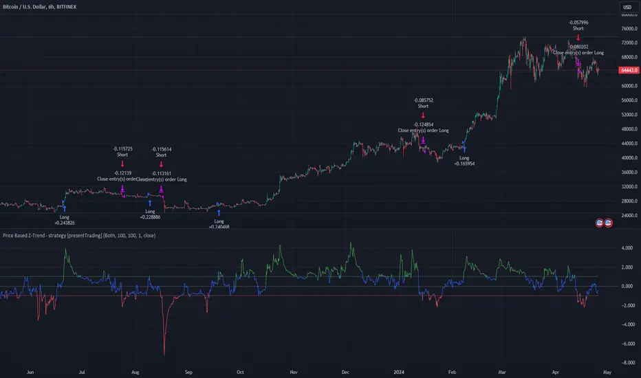
Price Based Z-Trend - Strategy [presentTrading]█ Introduction and How it is Different
Z-score: a statistical measurement of a score's relationship to the mean in a group of scores.
Simple but effective approach.
The "Price Based Z-Trend - Strategy " leverages the Z-score, a statistical measure that gauges the deviation of a price from its moving average, normalized against its standard deviation. This strategy stands out due to its simplicity and effectiveness, particularly in markets where price movements often revert to a mean. Unlike more complex systems that might rely on a multitude of indicators, the Z-Trend strategy focuses on clear, statistically significant price movements, making it ideal for traders who prefer a streamlined, data-driven approach.
BTCUSD 6h LS Performance
█ Strategy, How It Works: Detailed Explanation
🔶 Calculation of the Z-score
"Z-score is a statistical measurement that describes a value's relationship to the mean of a group of values. Z-score is measured in terms of standard deviations from the mean. If a Z-score is 0, it indicates that the data point's score is identical to the mean score. A Z-score of 1.0 would indicate a value that is one standard deviation from the mean. Z-scores may be positive or negative, with a positive value indicating the score is above the mean and a negative score indicating it is below the mean."
The Z-score is central to this strategy. It is calculated by taking the difference between the current price and the Exponential Moving Average (EMA) of the price over a user-defined length, then dividing this by the standard deviation of the price over the same length:
z = (x - μ) /σ
Local
🔶 Trading Signals
Trading signals are generated based on the Z-score crossing predefined thresholds:
- Long Entry: When the Z-score crosses above the positive threshold.
- Long Exit: When the Z-score falls below the negative threshold.
- Short Entry: When the Z-score falls below the negative threshold.
- Short Exit: When the Z-score rises above the positive threshold.
█ Trade Direction
The strategy allows users to select their preferred trading direction through an input option.
█ Usage
To use this strategy effectively, traders should first configure the Z-score thresholds according to their risk tolerance and market volatility. It's also crucial to adjust the length for the EMA and standard deviation calculations based on historical performance and the expected "noise" in price data.
The strategy is designed to be flexible, allowing traders to refine settings to better capture profitable opportunities in specific market conditions.
█ Default Settings
- Trade Direction: Both
- Standard Deviation Length: 100
- Average Length: 100
- Threshold for Z-score: 1.0
- Bar Color Indicator: Enabled
These settings offer a balanced starting point but can be customized to suit various trading styles and market environments. The strategy's parameters are designed to be adjusted as traders gain experience and refine their approach based on ongoing market analysis.
Z-score is a must-learn approach for every algorithmic trader.
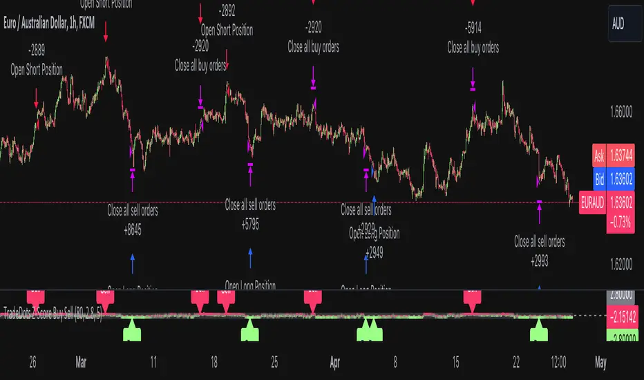
Buy Sell Strategy With Z-Score [TradeDots]The "Buy Sell Strategy With Z-Score" is a trading strategy that harnesses Z-Score statistical metrics to identify potential pricing reversals, for opportunistic buying and selling opportunities.
HOW DOES IT WORK
The strategy operates by calculating the Z-Score of the closing price for each candlestick. This allows us to evaluate how significantly the current price deviates from its typical volatility level.
The strategy first takes the scope of a rolling window, adjusted to the user's preference. This window is used to compute both the standard deviation and mean value. With these values, the strategic model finalizes the Z-Score. This determination is accomplished by subtracting the mean from the closing price and dividing the resulting value by the standard deviation.
This approach provides an estimation of the price's departure from its traditional trajectory, thereby identifying market conditions conducive to an asset being overpriced or underpriced.
APPLICATION
Firstly, it is better to identify a stable trading pair for this technique, such as two stocks with considerable correlation. This is to ensure conformance with the statistical model's assumption of a normal Gaussian distribution model. The ideal performance is theoretically situated within a sideways market devoid of skewness.
Following pair selection, the user should refine the span of the rolling window. A broader window smoothens the mean, more accurately capturing long-term market trends, while potentially enhancing volatility. This refinement results in fewer, yet precise trading signals.
Finally, the user must settle on an optimal Z-Score threshold, which essentially dictates the timing for buy/sell actions when the Z-Score exceeds with thresholds. A positive threshold signifies the price veering away from its mean, triggering a sell signal. Conversely, a negative threshold denotes the price falling below its mean, illustrating an underpriced condition that prompts a buy signal.
Within a normal distribution, a Z-Score of 1 records about 68% of occurrences centered at the mean, while a Z-Score of 2 captures approximately 95% of occurrences.
The 'cool down period' is essentially the number of bars that await before the next signal generation. This feature is employed to dodge the occurrence of multiple signals in a short period.
DEFAULT SETUP
The following is the default setup on EURUSD 1h timeframe
Rolling Window: 80
Z-Score Threshold: 2.8
Signal Cool Down Period: 5
Commission: 0.03%
Initial Capital: $10,000
Equity per Trade: 30%
RISK DISCLAIMER
Trading entails substantial risk, and most day traders incur losses. All content, tools, scripts, articles, and education provided by TradeDots serve purely informational and educational purposes. Past performances are not definitive predictors of future results.
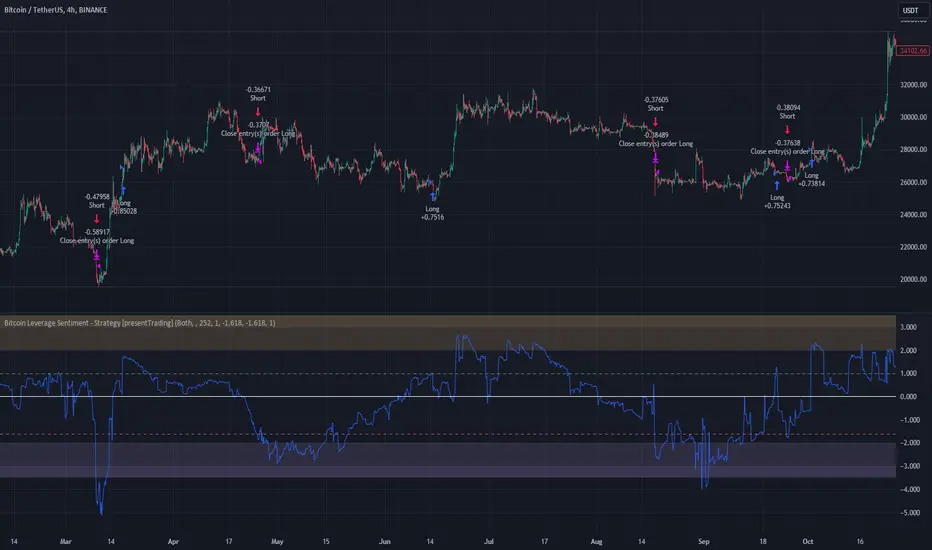
Bitcoin Leverage Sentiment - Strategy [presentTrading]█ Introduction and How it is Different
The "Bitcoin Leverage Sentiment - Strategy " represents a novel approach in the realm of cryptocurrency trading by focusing on sentiment analysis through leveraged positions in Bitcoin. Unlike traditional strategies that primarily rely on price action or technical indicators, this strategy leverages the power of Z-Score analysis to gauge market sentiment by examining the ratio of leveraged long to short positions. By assessing how far the current sentiment deviates from the historical norm, it provides a unique lens to spot potential reversals or continuation in market trends, making it an innovative tool for traders who wish to incorporate market psychology into their trading arsenal.
BTC 4h L/S Performance
local
█ Strategy, How It Works: Detailed Explanation
🔶 Data Collection and Ratio Calculation
Firstly, the strategy acquires data on leveraged long (**`priceLongs`**) and short positions (**`priceShorts`**) for Bitcoin. The primary metric of interest is the ratio of long positions relative to the total of both long and short positions:
BTC Ratio=priceLongs / (priceLongs+priceShorts)
This ratio reflects the prevailing market sentiment, where values closer to 1 indicate a bullish sentiment (dominance of long positions), and values closer to 0 suggest bearish sentiment (prevalence of short positions).
🔶 Z-Score Calculation
The Z-Score is then calculated to standardize the BTC Ratio, allowing for comparison across different time periods. The Z-Score formula is:
Z = (X - μ) / σ
Where:
- X is the current BTC Ratio.
- μ is the mean of the BTC Ratio over a specified period (**`zScoreCalculationPeriod`**).
- σ is the standard deviation of the BTC Ratio over the same period.
The Z-Score helps quantify how far the current sentiment deviates from the historical norm, with high positive values indicating extreme bullish sentiment and high negative values signaling extreme bearish sentiment.
🔶 Signal Generation: Trading signals are derived from the Z-Score as follows:
Long Entry Signal: Occurs when the BTC Ratio Z-Score crosses above the thresholdLongEntry, suggesting bullish sentiment.
- Condition for Long Entry = BTC Ratio Z-Score > thresholdLongEntry
Long Exit/Short Entry Signal: Triggered when the BTC Ratio Z-Score drops below thresholdLongExit for exiting longs or below thresholdShortEntry for entering shorts, indicating a shift to bearish sentiment.
- Condition for Long Exit/Short Entry = BTC Ratio Z-Score < thresholdLongExit or BTC Ratio Z-Score < thresholdShortEntry
Short Exit Signal: Happens when the BTC Ratio Z-Score exceeds the thresholdShortExit, hinting at reducing bearish sentiment and a potential switch to bullish conditions.
- Condition for Short Exit = BTC Ratio Z-Score > thresholdShortExit
🔶Implementation and Visualization: The strategy applies these conditions for trade management, aligning with the selected trade direction. It visualizes the BTC Ratio Z-Score with horizontal lines at entry and exit thresholds, illustrating the current sentiment against historical norms.
█ Trade Direction
The strategy offers flexibility in trade direction, allowing users to choose between long, short, or both, depending on their market outlook and risk tolerance. This adaptability ensures that traders can align the strategy with their individual trading style and market conditions.
█ Usage
To employ this strategy effectively:
1. Customization: Begin by setting the trade direction and adjusting the Z-Score calculation period and entry/exit thresholds to match your trading preferences.
2. Observation: Monitor the Z-Score and its moving average for potential trading signals. Look for crossover events relative to the predefined thresholds to identify entry and exit points.
3. Confirmation: Consider using additional analysis or indicators for signal confirmation, ensuring a comprehensive approach to decision-making.
█ Default Settings
- Trade Direction: Determines if the strategy engages in long, short, or both types of trades, impacting its adaptability to market conditions.
- Timeframe Input: Influences signal frequency and sensitivity, affecting the strategy's responsiveness to market dynamics.
- Z-Score Calculation Period: Affects the strategy’s sensitivity to market changes, with longer periods smoothing data and shorter periods increasing responsiveness.
- Entry and Exit Thresholds: Set the Z-Score levels for initiating or exiting trades, balancing between capturing opportunities and minimizing false signals.
- Impact of Default Settings: Provides a balanced approach to leverage sentiment trading, with adjustments needed to optimize performance across various market conditions.
Bollinger Bands StrategyBollinger Bands Strategy :
INTRODUCTION :
This strategy is based on the famous Bollinger Bands. These are constructed using a standard moving average (SMA) and the standard deviation of past prices. The theory goes that 90% of the time, the price is contained between these two bands. If it were to break out, this would mean either a reversal or a continuation. However, when a reversal occurs, the movement is weak, whereas when a continuation occurs, the movement is substantial and profits can be interesting. We're going to use BB to take advantage of this strong upcoming movement, while managing our risks reasonably. There's also a money management method for reinvesting part of the profits or reducing the size of orders in the event of substantial losses.
BOLLINGER BANDS :
The construction of Bollinger bands is straightforward. First, plot the SMA of the price, with a length specified by the user. Then calculate the standard deviation to measure price dispersion in relation to the mean, using this formula :
stdv = (((P1 - avg)^2 + (P2 - avg)^2 + ... + (Pn - avg)^2) / n)^1/2
To plot the two Bollinger bands, we then add a user-defined number of standard deviations to the initial SMA. The default is to add 2. The result is :
Upper_band = SMA + 2*stdv
Lower_band = SMA - 2*stdv
When the price leaves this channel defined by the bands, we obtain buy and sell signals.
PARAMETERS :
BB Length : This is the length of the Bollinger Bands, i.e. the length of the SMA used to plot the bands, and the length of the price series used to calculate the standard deviation. The default is 120.
Standard Deviation Multipler : adds or subtracts this number of times the standard deviation from the initial SMA. Default is 2.
SMA Exit Signal Length : Exit signals for winning and losing trades are triggered by another SMA. This parameter defines the length of this SMA. The default is 110.
Max Risk per trade (in %) : It's the maximum percentage the user can lose in one trade. The default is 6%.
Fixed Ratio : This is the amount of gain or loss at which the order quantity is changed. The default is 400, meaning that for each $400 gain or loss, the order size is increased or decreased by a user-selected amount.
Increasing Order Amount : This is the amount to be added to or subtracted from orders when the fixed ratio is reached. The default is $200, which means that for every $400 gain, $200 is reinvested in the strategy. On the other hand, for every $400 loss, the order size is reduced by $200.
Initial capital : $1000
Fees : Interactive Broker fees apply to this strategy. They are set at 0.18% of the trade value.
Slippage : 3 ticks or $0.03 per trade. Corresponds to the latency time between the moment the signal is received and the moment the order is executed by the broker.
Important : A bot has been used to test the different parameters and determine which ones maximize return while limiting drawdown. This strategy is the most optimal on BITSTAMP:BTCUSD in 8h timeframe with the following parameters :
BB Length = 120
Standard Deviation Multipler = 2
SMA Exit Signal Length = 110
Max Risk per trade (in %) = 6%
ENTER RULES :
The entry rules are simple:
If close > Upper_band it's a LONG signal
If close < Lower_band it's a SHORT signal
EXIT RULES :
If we are LONG and close < SMA_EXIT, position is closed
If we are SHORT and close > SMA_EXIT, the position is closed
Positions close automatically if they lose more than 6% to limit risk
RISK MANAGEMENT :
This strategy is subject to losses. We manage our risk using the exit SMA or using a SL sets to 6%. This SMA gives us exit signals when the price closes below or above, thus limiting losses. If the signal arrives too late, the position is closed after a loss of 6%.
MONEY MANAGEMENT :
The fixed ratio method was used to manage our gains and losses. For each gain of an amount equal to the fixed ratio value, we increase the order size by a value defined by the user in the "Increasing order amount" parameter. Similarly, each time we lose an amount equal to the value of the fixed ratio, we decrease the order size by the same user-defined value. This strategy increases both performance and drawdown.
NOTE :
Please note that the strategy is backtested from 2017-01-01. As the timeframe is 8h, this strategy is a medium/long-term strategy. That's why only 51 trades were closed. Be careful, as the test sample is small and performance may not necessarily reflect what may happen in the future.
Enjoy the strategy and don't forget to take the trade :)

VWAP Trendfollow Strategy [wbburgin]This is an experimental strategy that enters long when the instrument crosses over the upper standard deviation band of a VWAP and enters short when the instrument crosses below the bottom standard deviation band of the VWAP. I have added a trend filter as well, which stops entries that are opposite to the current trend of the VWAP. The trend filter will reduce total false breakouts, thus improving the % profitable while maintaining the overall returns of the strategy. Because this is a trend-following breakout strategy, the % profitable will typically be low but the average % return will be higher. As a rule, be sure to look at the average winning trade % compared to the average losing trade %, and compare that to the % profitable to judge the effectiveness of a strategy. Factor in fees and slippage as well.
This strategy appears to work better with the lower timeframes, and I was impressed with its results. It also appears to work on a wide range of asset classes. There isn't a stop loss or take profit built-in (other than the reversal signals, which close the current trade), so I would encourage you to expand on the strategy based on your own trading parameters.
You can toggle off the bar colors and the trend filter if you so desire.
Future updates to this script (or ideas of improving on it) might include a take profit level set at one standard deviation past the current level and a stop loss level set at one standard deviation closer to the vwap from the current level - or applying a multiple to the two based off of your reward/risk ratio.
About the strategy results below: this is with commissions of 0.5 % per trade.

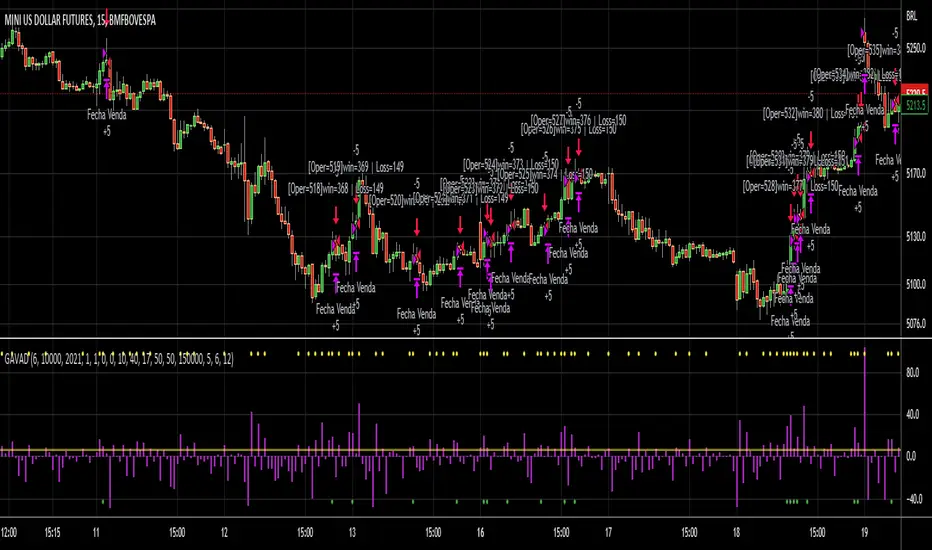
GAVAD - Selling after a Strong MovimentThis strategy search for a moment whe the market make two candles are consistently strong, and open a Sell, searching the imediactly correction, on the new candle. It`s easy to see the bars on the histogram graph. Purple Bars represent the candle variation. when on candle cross ove the Signal line the graph plot an Yellow ci, if the second bar crossover the signal a green circle is ploted and the operation start on start of the next candle.
This strategy can be used in a lot of Stocks and other graphs. many times we need a small time of graph, maybe 1 or 5 minutes because the gain shoud be planned to a midle of the second candle. You need look the stocks you will use.
Stocks > 100 dolars isnt great, markets extremly volatly not too. but, Stocks that have a consistently development are very interisting. Look to markets searching maybe 0.5% or 1%.
For this moment, I make the development of a Brasilian Real x American Dollar. In 15 Minutes.
if you use in small timeframe the results can be better.
On this time we make more than 500 trades with a small lot of contracts, without a big percent profitable, but a small profit in each operation, maybe you search more than. To present a real trading system I insert a spreed to present a correct view of the results.
Each stock, Index, or crypto there is a specific configuration?
my suggestion for new stocks
You need choice a stock and using the setup search set over than 70% gain (percent profitable), using a 1% of gain and loss between 1-2%
as the exemple (WDO)
default I prepare a Brazilian Index
6-signal (6% is variation of a candle of the last candle)
10000- multiplicator (its important to configure diferences betwen a stock and an Indice)
gain 3 (this proportion will be set looking you target, how I say, 1% can be good)
loss 8 (this proportion will be set with you bankroll management, how I say, maybe 2%, you need evaluate)
for maximize operations I use in the 1 or 5 minute graph. Timeframes more large make slowlly results,
(but not unable that you use in a 1 hour or a 1 day.)
I make this script by zero. Maybe the code doesnt so organized, but is very easy to understand. If you have any doubts . leave a comment.
I hope help you.
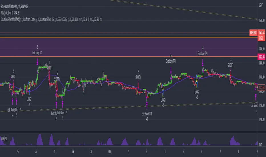
Gaussian Filter ModifiedAn effort to enhance auto-trading based on Gaussian Filter with Standard Deviation Filtering, Trading True Range and Smoothed SMA was added to remove noise contributing to ranging markets and unwanted entries against established trend.
Gaussian parameters need to be adjusted for different asset pair to find its own "signature", then filter out bad entry with TTR and SMA.
*Credits to Loxx for his work on Gaussian Filter
Quantitative mean reversion v4The code uses the concept of mean reversion. Mean reversion suggests that price over a period of time reverts back to its statistical mean. In simple terms, it means if a price has drifted apart from the statistical mean, after a certain amount of time, it will revert back to its statistical mean. This drift is measured via z-score. When the z-score value is high, the price is expected to revert. Besides, the higher the time frame you use, the lesser the drift is, so reduce the z-score in the tabs if you use higher time frames, else, vice-versa.
Based on the parameters, the code will provide a trade signal - both long and short, and entry and exit. You can use notifications for alerts. Please use the parameters in the options to find the best combinations for your stocks.
In the properties, you can use your own brokers commission, capital, to see if the strategy is profitable for your ticker in the long run or not. This code has been tested for profits for various assets in both crypto - Bitcoin futures , Ethereum futures -, and stocks - AMD , Apple , MSFT , etc.
This is not get rich quick scheme, and you have to be patient with it for the long run.
If you have any query, please feel free to ask in the comments sections.
If you want some new changes, please feel free to suggest
Currently, I am optimising the maximum time for holding a trade. Till that's completed, use this and please feel free to leave a feedback to make it better

STD-Filtered, Gaussian-Kernel-Weighted Moving Average BT [Loxx]STD-Filtered, Gaussian-Kernel-Weighted Moving Average BT is the backtest for the following indicator
Included:
This backtest uses a special implementation of ATR and ATR smoothing called "True Range Double" which is a range calculation that accounts for volatility skew.
You can set the backtest to 1-2 take profits with stop-loss
Signals can't exit on the same candle as the entry, this is coded in a way for 1-candle delay post entry
This should be coupled with the INDICATOR version linked above for the alerts and signals. Strategies won't paint the signal "L" or "S" until the entry actually happens, but indicators allow this, which is repainting on current candle, but this is an FYI if you want to get serious with Pinescript algorithmic botting
You can restrict the backtest by dates
It is advised that you understand what Heikin-Ashi candles do to strategies, the default settings for this backtest is NON Heikin-Ashi candles but you have the ability to change that in the source selection
This is a mathematically heavy, heavy-lifting strategy. Make sure you do your own research so you understand what is happening here.
STD-Filtered, Gaussian-Kernel-Weighted Moving Average is a moving average that weights price by using a Gaussian kernel function to calculate data points. This indicator also allows for filtering both source input price and output signal using a standard deviation filter.
Purpose
This purpose of this indicator is to take the concept of Kernel estimation and apply it in a way where instead of predicting past values, the weighted function predicts the current bar value at each bar to create a moving average that is suitable for trading. Normally this method is used to create an array of past estimators to model past data but this method is not useful for trading as the past values will repaint. This moving average does NOT repaint, however you much allow signals to close on the current bar before taking the signal. You can compare this to Nadaraya-Watson Estimator wherein they use Nadaraya-Watson estimator method with normalized kernel weighted function to model price.
What are Kernel Functions?
A kernel function is used as a weighing function to develop non-parametric regression model is discussed. In the beginning of the article, a brief discussion about properties of kernel functions and steps to build kernels around data points are presented.
Kernel Function
In non-parametric statistics, a kernel is a weighting function which satisfies the following properties.
A kernel function must be symmetrical. Mathematically this property can be expressed as K (-u) = K (+u). The symmetric property of kernel function enables its maximum value (max(K(u)) to lie in the middle of the curve.
The area under the curve of the function must be equal to one. Mathematically, this property is expressed as: integral −∞ + ∞ ∫ K(u)d(u) = 1
Value of kernel function can not be negative i.e. K(u) ≥ 0 for all −∞ < u < ∞.
Kernel Estimation
In this article, Gaussian kernel function is used to calculate kernels for the data points. The equation for Gaussian kernel is:
K(u) = (1 / sqrt(2pi)) * e^(-0.5 *(j / bw )^2)
Where xi is the observed data point. j is the value where kernel function is computed and bw is called the bandwidth. Bandwidth in kernel regression is called the smoothing parameter because it controls variance and bias in the output.
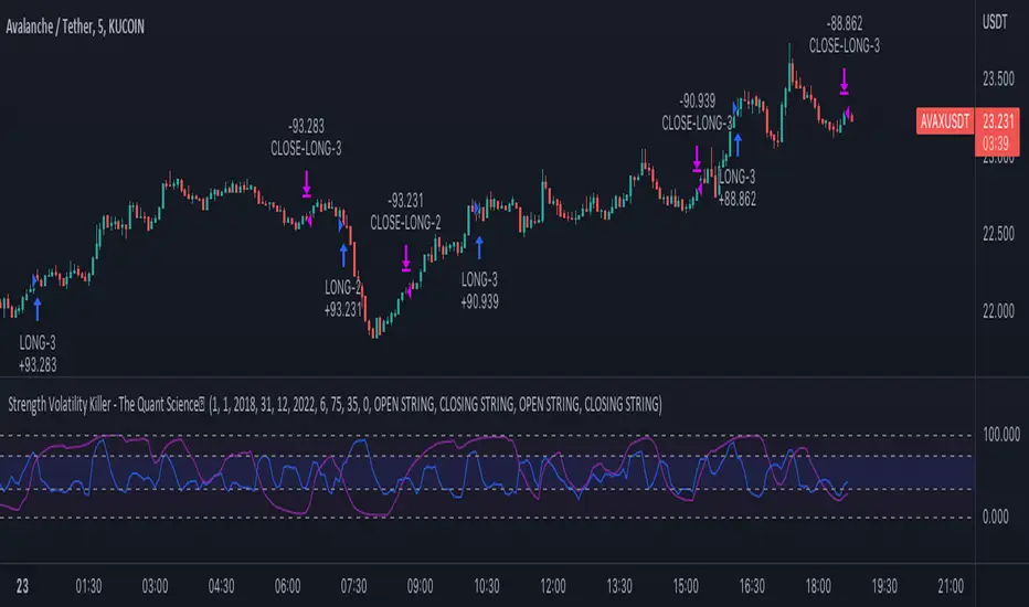
Strength Volatility Killer - The Quant ScienceStrength Volatility Killer - The Quant Science™ is based on a special version of RSI (Relative Strength Index), created with the simple average and standard deviation.
DESCRIPTION
The algorithm analyses the market and opens positions following three different volatility entry conditions. Each entry has a specific and personal exit condition. The user can setting trailing stop loss from user interface.
USER INTERFACE SETTING
Configures the algorithm from the user interface.
AUTO TRADING COMPLIANT
With the user interface, the trader can easily set up this algorithm for automatic trading.
BACKTESTING INCLUDED
The trader can adjust the backtesting period of the strategy before putting it live. Analyze large periods such as years or months or focus on short-term periods.
NO LIMIT TIMEFRAME
This algorithm can be used on all timeframes.
GENERAL FEATURES
Multi-strategy: the algorithm can apply long strategy or short strategy.
Built-in alerts: the algorithm contains alerts that can be customized from the user interface.
Integrated indicator: indicator is included.
Backtesting included: quickly automatic backtesting of the strategy.
Auto-trading compliant: functions for auto trading are included.
ABOUT BACKTESTING
Backtesting refers to the period 13 June 2022 - today, ticker: AVAX/USDT, timeframe 5 minutes.
Initial capital: $1000.00
Commission per trade: 0.03%
STD-Filterd, R-squared Adaptive T3 w/ Dynamic Zones BT [Loxx]STD-Filterd, R-squared Adaptive T3 w/ Dynamic Zones BT is the backtest strategy for "STD-Filterd, R-squared Adaptive T3 w/ Dynamic Zones " seen below:
Included:
This backtest uses a special implementation of ATR and ATR smoothing called "True Range Double" which is a range calculation that accounts for volatility skew.
You can set the backtest to 1-2 take profits with stop-loss
Signals can't exit on the same candle as the entry, this is coded in a way for 1-candle delay post entry
This should be coupled with the INDICATOR version linked above for the alerts and signals. Strategies won't paint the signal "L" or "S" until the entry actually happens, but indicators allow this, which is repainting on current candle, but this is an FYI if you want to get serious with Pinescript algorithmic botting
You can restrict the backtest by dates
It is advised that you understand what Heikin-Ashi candles do to strategies, the default settings for this backtest is NON Heikin-Ashi candles but you have the ability to change that in the source selection
This is a mathematically heavy, heavy-lifting strategy with multi-layered adaptivity. Make sure you do your own research so you understand what is happening here. This can be used as its own trading system without any other oscillators, moving average baselines, or volatility/momentum confirmation indicators.
What is the T3 moving average?
Better Moving Averages Tim Tillson
November 1, 1998
Tim Tillson is a software project manager at Hewlett-Packard, with degrees in Mathematics and Computer Science. He has privately traded options and equities for 15 years.
Introduction
"Digital filtering includes the process of smoothing, predicting, differentiating, integrating, separation of signals, and removal of noise from a signal. Thus many people who do such things are actually using digital filters without realizing that they are; being unacquainted with the theory, they neither understand what they have done nor the possibilities of what they might have done."
This quote from R. W. Hamming applies to the vast majority of indicators in technical analysis . Moving averages, be they simple, weighted, or exponential, are lowpass filters; low frequency components in the signal pass through with little attenuation, while high frequencies are severely reduced.
"Oscillator" type indicators (such as MACD , Momentum, Relative Strength Index ) are another type of digital filter called a differentiator.
Tushar Chande has observed that many popular oscillators are highly correlated, which is sensible because they are trying to measure the rate of change of the underlying time series, i.e., are trying to be the first and second derivatives we all learned about in Calculus.
We use moving averages (lowpass filters) in technical analysis to remove the random noise from a time series, to discern the underlying trend or to determine prices at which we will take action. A perfect moving average would have two attributes:
It would be smooth, not sensitive to random noise in the underlying time series. Another way of saying this is that its derivative would not spuriously alternate between positive and negative values.
It would not lag behind the time series it is computed from. Lag, of course, produces late buy or sell signals that kill profits.
The only way one can compute a perfect moving average is to have knowledge of the future, and if we had that, we would buy one lottery ticket a week rather than trade!
Having said this, we can still improve on the conventional simple, weighted, or exponential moving averages. Here's how:
Two Interesting Moving Averages
We will examine two benchmark moving averages based on Linear Regression analysis.
In both cases, a Linear Regression line of length n is fitted to price data.
I call the first moving average ILRS, which stands for Integral of Linear Regression Slope. One simply integrates the slope of a linear regression line as it is successively fitted in a moving window of length n across the data, with the constant of integration being a simple moving average of the first n points. Put another way, the derivative of ILRS is the linear regression slope. Note that ILRS is not the same as a SMA ( simple moving average ) of length n, which is actually the midpoint of the linear regression line as it moves across the data.
We can measure the lag of moving averages with respect to a linear trend by computing how they behave when the input is a line with unit slope. Both SMA (n) and ILRS(n) have lag of n/2, but ILRS is much smoother than SMA .
Our second benchmark moving average is well known, called EPMA or End Point Moving Average. It is the endpoint of the linear regression line of length n as it is fitted across the data. EPMA hugs the data more closely than a simple or exponential moving average of the same length. The price we pay for this is that it is much noisier (less smooth) than ILRS, and it also has the annoying property that it overshoots the data when linear trends are present.
However, EPMA has a lag of 0 with respect to linear input! This makes sense because a linear regression line will fit linear input perfectly, and the endpoint of the LR line will be on the input line.
These two moving averages frame the tradeoffs that we are facing. On one extreme we have ILRS, which is very smooth and has considerable phase lag. EPMA has 0 phase lag, but is too noisy and overshoots. We would like to construct a better moving average which is as smooth as ILRS, but runs closer to where EPMA lies, without the overshoot.
A easy way to attempt this is to split the difference, i.e. use (ILRS(n)+EPMA(n))/2. This will give us a moving average (call it IE /2) which runs in between the two, has phase lag of n/4 but still inherits considerable noise from EPMA. IE /2 is inspirational, however. Can we build something that is comparable, but smoother? Figure 1 shows ILRS, EPMA, and IE /2.
Filter Techniques
Any thoughtful student of filter theory (or resolute experimenter) will have noticed that you can improve the smoothness of a filter by running it through itself multiple times, at the cost of increasing phase lag.
There is a complementary technique (called twicing by J.W. Tukey) which can be used to improve phase lag. If L stands for the operation of running data through a low pass filter, then twicing can be described by:
L' = L(time series) + L(time series - L(time series))
That is, we add a moving average of the difference between the input and the moving average to the moving average. This is algebraically equivalent to:
2L-L(L)
This is the Double Exponential Moving Average or DEMA , popularized by Patrick Mulloy in TASAC (January/February 1994).
In our taxonomy, DEMA has some phase lag (although it exponentially approaches 0) and is somewhat noisy, comparable to IE /2 indicator.
We will use these two techniques to construct our better moving average, after we explore the first one a little more closely.
Fixing Overshoot
An n-day EMA has smoothing constant alpha=2/(n+1) and a lag of (n-1)/2.
Thus EMA (3) has lag 1, and EMA (11) has lag 5. Figure 2 shows that, if I am willing to incur 5 days of lag, I get a smoother moving average if I run EMA (3) through itself 5 times than if I just take EMA (11) once.
This suggests that if EPMA and DEMA have 0 or low lag, why not run fast versions (eg DEMA (3)) through themselves many times to achieve a smooth result? The problem is that multiple runs though these filters increase their tendency to overshoot the data, giving an unusable result. This is because the amplitude response of DEMA and EPMA is greater than 1 at certain frequencies, giving a gain of much greater than 1 at these frequencies when run though themselves multiple times. Figure 3 shows DEMA (7) and EPMA(7) run through themselves 3 times. DEMA^3 has serious overshoot, and EPMA^3 is terrible.
The solution to the overshoot problem is to recall what we are doing with twicing:
DEMA (n) = EMA (n) + EMA (time series - EMA (n))
The second term is adding, in effect, a smooth version of the derivative to the EMA to achieve DEMA . The derivative term determines how hot the moving average's response to linear trends will be. We need to simply turn down the volume to achieve our basic building block:
EMA (n) + EMA (time series - EMA (n))*.7;
This is algebraically the same as:
EMA (n)*1.7-EMA( EMA (n))*.7;
I have chosen .7 as my volume factor, but the general formula (which I call "Generalized Dema") is:
GD (n,v) = EMA (n)*(1+v)-EMA( EMA (n))*v,
Where v ranges between 0 and 1. When v=0, GD is just an EMA , and when v=1, GD is DEMA . In between, GD is a cooler DEMA . By using a value for v less than 1 (I like .7), we cure the multiple DEMA overshoot problem, at the cost of accepting some additional phase delay. Now we can run GD through itself multiple times to define a new, smoother moving average T3 that does not overshoot the data:
T3(n) = GD ( GD ( GD (n)))
In filter theory parlance, T3 is a six-pole non-linear Kalman filter. Kalman filters are ones which use the error (in this case (time series - EMA (n)) to correct themselves. In Technical Analysis , these are called Adaptive Moving Averages; they track the time series more aggressively when it is making large moves.
What is R-squared Adaptive?
One tool available in forecasting the trendiness of the breakout is the coefficient of determination ( R-squared ), a statistical measurement.
The R-squared indicates linear strength between the security's price (the Y - axis) and time (the X - axis). The R-squared is the percentage of squared error that the linear regression can eliminate if it were used as the predictor instead of the mean value. If the R-squared were 0.99, then the linear regression would eliminate 99% of the error for prediction versus predicting closing prices using a simple moving average .
R-squared is used here to derive a T3 factor used to modify price before passing price through a six-pole non-linear Kalman filter.
What are Dynamic Zones?
As explained in "Stocks & Commodities V15:7 (306-310): Dynamic Zones by Leo Zamansky, Ph .D., and David Stendahl"
Most indicators use a fixed zone for buy and sell signals. Here’ s a concept based on zones that are responsive to past levels of the indicator.
One approach to active investing employs the use of oscillators to exploit tradable market trends. This investing style follows a very simple form of logic: Enter the market only when an oscillator has moved far above or below traditional trading lev- els. However, these oscillator- driven systems lack the ability to evolve with the market because they use fixed buy and sell zones. Traders typically use one set of buy and sell zones for a bull market and substantially different zones for a bear market. And therein lies the problem.
Once traders begin introducing their market opinions into trading equations, by changing the zones, they negate the system’s mechanical nature. The objective is to have a system automatically define its own buy and sell zones and thereby profitably trade in any market — bull or bear. Dynamic zones offer a solution to the problem of fixed buy and sell zones for any oscillator-driven system.
An indicator’s extreme levels can be quantified using statistical methods. These extreme levels are calculated for a certain period and serve as the buy and sell zones for a trading system. The repetition of this statistical process for every value of the indicator creates values that become the dynamic zones. The zones are calculated in such a way that the probability of the indicator value rising above, or falling below, the dynamic zones is equal to a given probability input set by the trader.
To better understand dynamic zones, let's first describe them mathematically and then explain their use. The dynamic zones definition:
Find V such that:
For dynamic zone buy: P{X <= V}=P1
For dynamic zone sell: P{X >= V}=P2
where P1 and P2 are the probabilities set by the trader, X is the value of the indicator for the selected period and V represents the value of the dynamic zone.
The probability input P1 and P2 can be adjusted by the trader to encompass as much or as little data as the trader would like. The smaller the probability, the fewer data values above and below the dynamic zones. This translates into a wider range between the buy and sell zones. If a 10% probability is used for P1 and P2, only those data values that make up the top 10% and bottom 10% for an indicator are used in the construction of the zones. Of the values, 80% will fall between the two extreme levels. Because dynamic zone levels are penetrated so infrequently, when this happens, traders know that the market has truly moved into overbought or oversold territory.
Calculating the Dynamic Zones
The algorithm for the dynamic zones is a series of steps. First, decide the value of the lookback period t. Next, decide the value of the probability Pbuy for buy zone and value of the probability Psell for the sell zone.
For i=1, to the last lookback period, build the distribution f(x) of the price during the lookback period i. Then find the value Vi1 such that the probability of the price less than or equal to Vi1 during the lookback period i is equal to Pbuy. Find the value Vi2 such that the probability of the price greater or equal to Vi2 during the lookback period i is equal to Psell. The sequence of Vi1 for all periods gives the buy zone. The sequence of Vi2 for all periods gives the sell zone.
In the algorithm description, we have: Build the distribution f(x) of the price during the lookback period i. The distribution here is empirical namely, how many times a given value of x appeared during the lookback period. The problem is to find such x that the probability of a price being greater or equal to x will be equal to a probability selected by the user. Probability is the area under the distribution curve. The task is to find such value of x that the area under the distribution curve to the right of x will be equal to the probability selected by the user. That x is the dynamic zone.
Included:
Bar coloring
Signals
Alerts
Loxx's Expanded Source Types
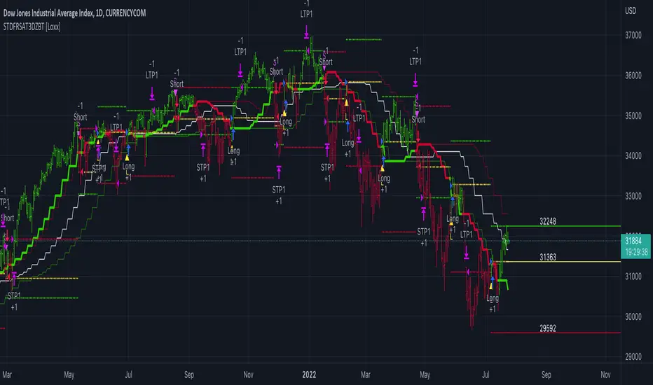
Cyatophilum VWAP StrategyAn indicator to backtest and automate VWAP custom strategies.
Use the Trend Mode to create Swing Trading strategies or Rotation Mode for Intraday Trading.
Configure your strategy using the Entry Condition Builder and Risk Management features, such as Trailing Stop & Take Profits, Safety Orders, and VWAP Exit conditions.
═════════════════════════════════════════════════════════════════════════
█ HOW IT WORKS
VWAP stands for Volume Weighted Average Price.
It is like a simple moving average that takes volume into account.
It is used by a lot of traders since it has everything one needs to know: price and volume.
The cummulated volume calculation resets every session, which interval can be configured.
From that we can calculate the MVWAP and the Standard Deviation Bands and create strategies around that.
█ HOW TO USE
Trend Mode
Trend Mode is the name for strategies built upon VWAP and price/MVWAP cross, most often for Swing Trading on high timeframes trending markets.
The side traded is often long and trying to beat Buy & Hold.
The trade exit can be triggered by a reversal signal (top chart), or a trailing stop (bottom chart) and take profit.
Rotation Mode
This is the mode for Intraday on low timeframes. It will work best on ranging markets.
We use the Standard Deviation Bands to buy/sell the price at overbougth/oversold levels.
The indicator allows to create complex entry conditions such as "Break out of 3rd bands AND break back in 2nd bands" within a certain amount of time.
We will use either the exit options to close the trade when prices reach an opposite band, or the risk management features explained below.
█ FEATURES
• VWAP settings
Configure the VWAP.
• Entry settings
Choose to go long, short, and if the strategy should reverse or not.
• Trend Mode
Choose to create entries from VWAP cross with price or MVWAP.
• Rotation Mode
Configure the 3 bands and build a condition for entry. The multiple inputs allow to add up different events required to trigger an entry, using 3 logical gates that can be linked together using a AND or OR condition. The events being: "break out", "Break back in" or "Just touches" any of the 3 bands. The condition must be met within a certain period of time to be valid.
• Exit settings
Options to exit trades at the end of every session or when the price reaches an opposite band.
• Stop Loss & Take Profit
Configure your stop loss and take profit for long and short trades.
You can also make a trailing stoploss and a trailing take profit.
• Safety Orders (DCA)
Create a strategy with up to 100 safety orders.
Configure their placement and order size using the price deviation, step scale, take profit type (from base order or total volume), and volume scale settings.
Graphics
A Configuration panel with all the indicator settings, useful for sharing a strategy.
A Backtest Results panel with buy & Hold Comparator.
█ ALERTS
Configure your alert messages for all events in the indicator settings.
Then click "Add Alert". In the popup window, select the option "alert() function calls only", give the alert a name and you are good to go!
█ BACKTEST RESULTS
The backtest settings used in this snapshot are the following:
Initial Capital: 10 000€
Order size: 10% equity
Commission: 0.1€ per order
Slippage : 10 ticks
Please read the author instructions below for access.
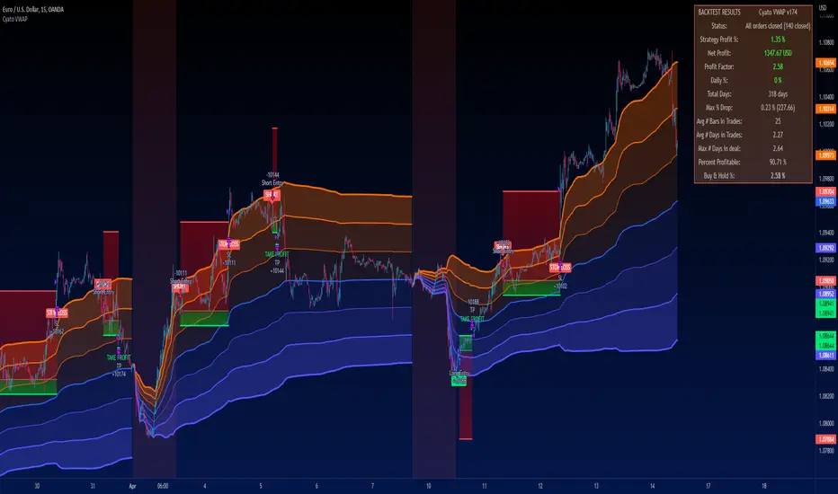
[KL] Double Bollinger Bands Strategy (for Crypto/FOREX)This strategy uses a setup consisting of two Bollinger Bands based on the 20 period 20-SMA +/-
(a) upper/lower bands of two standard deviations apart, and
(b) upper/lower bands of one standard deviation apart.
We consider price at +/- one standard deviation apart from 20-SMA as the "Neutral Zone".
If price closes above Neutral Zone after a period of consolidation, then it's an opportunity for entry. Strategy will long, anticipating for breakout.
The illustration below shows price closing above the Neutral Zone after a period of consolidation.
a.c-dn.net
Position is exited when prices closes at Neutral Zone (being lower than prior bars)
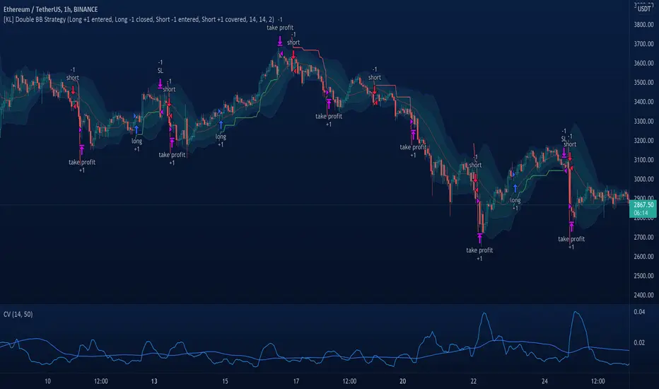
[KL] Bollinger Bands Consolidation StrategyThis strategy will enter into long position based on the volatility of prices implied by indicators of (a) Bollinger bands, and (b) ATR.
Application of Bollinger bands ("BOLL")
Using plain vanilla settings for BOLL (i.e. 20 period moving average, and 2 standard deviations of closing prices), we are interested to know about the shape of the area that is bounded by the upper and lower bands.
In theory, consolidation happens when volatility of price decreases. Visually speaking, this is represented by the narrowing of the upper/lower bands. This strategy considers the narrowing of BOLL bands as the primary indicator for long-entry.
Application of ATRs (as confirmations)
Firstly, to confirm that BOLL bands are narrowing (as mentioned above), the ATR at a potential point of entry is compared against the standard deviation of prices over BOLL's lookback periods. Once again, visualizing the shape of BOLL bands during consolidation, we assume the lines begin to squeeze when the distance between the center line and upper/lower band is less than two current ATRs.
Secondly, this strategy looks into the moving average of ATRs to assure that prices are not too choppy when entering into market. If the moving average of ATR decreases at a point in time such that all the above conditions are met, then we can assert that the volatility of price is decreasing.
Thirdly, ATR is used for determining the size of our trailing stop loss. We will keep the multiplier fixed at two.