KalmanfilterLibrary "Kalmanfilter"
A sophisticated Kalman Filter implementation for financial time series analysis
@author Rocky-Studio
@version 1.0
initialize(initial_value, process_noise, measurement_noise)
Initializes Kalman Filter parameters
Parameters:
initial_value (float) : (float) The initial state estimate
process_noise (float) : (float) The process noise coefficient (Q)
measurement_noise (float) : (float) The measurement noise coefficient (R)
Returns: A tuple containing
update(prev_state, prev_covariance, measurement, process_noise, measurement_noise)
Update Kalman Filter state
Parameters:
prev_state (float)
prev_covariance (float)
measurement (float)
process_noise (float)
measurement_noise (float)
calculate_measurement_noise(price_series, length)
Adaptive measurement noise calculation
Parameters:
price_series (array)
length (int)
calculate_measurement_noise_simple(price_series)
Parameters:
price_series (array)
update_trading(prev_state, prev_velocity, prev_covariance, measurement, volatility_window)
Enhanced trading update with velocity
Parameters:
prev_state (float)
prev_velocity (float)
prev_covariance (float)
measurement (float)
volatility_window (int)
model4_update(prev_mean, prev_speed, prev_covariance, price, process_noise, measurement_noise)
Kalman Filter Model 4 implementation (Benhamou 2018)
Parameters:
prev_mean (float)
prev_speed (float)
prev_covariance (array)
price (float)
process_noise (array)
measurement_noise (float)
model4_initialize(initial_price)
Initialize Model 4 parameters
Parameters:
initial_price (float)
model4_default_process_noise()
Create default process noise matrix for Model 4
model4_calculate_measurement_noise(price_series, length)
Adaptive measurement noise calculation for Model 4
Parameters:
price_series (array)
length (int)
Statistics

Request█ OVERVIEW
This library is a tool for Pine Script™ programmers that consolidates access to a wide range of lesser-known data feeds available on TradingView, including metrics from the FRED database, FINRA short sale volume, open interest, and COT data. The functions in this library simplify requests for these data feeds, making them easier to retrieve and use in custom scripts.
█ CONCEPTS
Federal Reserve Economic Data (FRED)
FRED (Federal Reserve Economic Data) is a comprehensive online database curated by the Federal Reserve Bank of St. Louis. It provides free access to extensive economic and financial data from U.S. and international sources. FRED includes numerous economic indicators such as GDP, inflation, employment, and interest rates. Additionally, it provides financial market data, regional statistics, and international metrics such as exchange rates and trade balances.
Sourced from reputable organizations, including U.S. government agencies, international institutions, and other public and private entities, FRED enables users to analyze over 825,000 time series, download their data in various formats, and integrate their information into analytical tools and programming workflows.
On TradingView, FRED data is available from ticker identifiers with the "FRED:" prefix. Users can search for FRED symbols in the "Symbol Search" window, and Pine scripts can retrieve data for these symbols via `request.*()` function calls.
FINRA Short Sale Volume
FINRA (the Financial Industry Regulatory Authority) is a non-governmental organization that supervises and regulates U.S. broker-dealers and securities professionals. Its primary aim is to protect investors and ensure integrity and transparency in financial markets.
FINRA's Short Sale Volume data provides detailed information about daily short-selling activity across U.S. equity markets. This data tracks the volume of short sales reported to FINRA's trade reporting facilities (TRFs), including shares sold on FINRA-regulated Alternative Trading Systems (ATSs) and over-the-counter (OTC) markets, offering transparent access to short-selling information not typically available from exchanges. This data helps market participants, researchers, and regulators monitor trends in short-selling and gain insights into bearish sentiment, hedging strategies, and potential market manipulation. Investors often use this data alongside other metrics to assess stock performance, liquidity, and overall trading activity.
It is important to note that FINRA's Short Sale Volume data does not consolidate short sale information from public exchanges and excludes trading activity that is not publicly disseminated.
TradingView provides ticker identifiers for requesting Short Sale Volume data with the format "FINRA:_SHORT_VOLUME", where "" is a supported U.S. equities symbol (e.g., "AAPL").
Open Interest (OI)
Open interest is a cornerstone indicator of market activity and sentiment in derivatives markets such as options or futures. In contrast to volume, which measures the number of contracts opened or closed within a period, OI measures the number of outstanding contracts that are not yet settled. This distinction makes OI a more robust indicator of how money flows through derivatives, offering meaningful insights into liquidity, market interest, and trends. Many traders and investors analyze OI alongside volume and price action to gain an enhanced perspective on market dynamics and reinforce trading decisions.
TradingView offers many ticker identifiers for requesting OI data with the format "_OI", where "" represents a derivative instrument's ticker ID (e.g., "COMEX:GC1!").
Commitment of Traders (COT)
Commitment of Traders data provides an informative weekly breakdown of the aggregate positions held by various market participants, including commercial hedgers, non-commercial speculators, and small traders, in the U.S. derivative markets. Tallied and managed by the Commodity Futures Trading Commission (CFTC) , these reports provide traders and analysts with detailed insight into an asset's open interest and help them assess the actions of various market players. COT data is valuable for gaining a deeper understanding of market dynamics, sentiment, trends, and liquidity, which helps traders develop informed trading strategies.
TradingView has numerous ticker identifiers that provide access to time series containing data for various COT metrics. To learn about COT ticker IDs and how they work, see our LibraryCOT publication.
█ USING THE LIBRARY
Common function characteristics
• This library's functions construct ticker IDs with valid formats based on their specified parameters, then use them as the `symbol` argument in request.security() to retrieve data from the specified context.
• Most of these functions automatically select the timeframe of a data request because the data feeds are not available for all timeframes.
• All the functions have two overloads. The first overload of each function uses values with the "simple" qualifier to define the requested context, meaning the context does not change after the first script execution. The second accepts "series" values, meaning it can request data from different contexts across executions.
• The `gaps` parameter in most of these functions specifies whether the returned data is `na` when a new value is unavailable for request. By default, its value is `false`, meaning the call returns the last retrieved data when no new data is available.
• The `repaint` parameter in applicable functions determines whether the request can fetch the latest unconfirmed values from a higher timeframe on realtime bars, which might repaint after the script restarts. If `false`, the function only returns confirmed higher-timeframe values to avoid repainting. The default value is `true`.
`fred()`
The `fred()` function retrieves the most recent value of a specified series from the Federal Reserve Economic Data (FRED) database. With this function, programmers can easily fetch macroeconomic indicators, such as GDP and unemployment rates, and use them directly in their scripts.
How it works
The function's `fredCode` parameter accepts a "string" representing the unique identifier of a specific FRED series. Examples include "GDP" for the "Gross Domestic Product" series and "UNRATE" for the "Unemployment Rate" series. Over 825,000 codes are available. To access codes for available series, search the FRED website .
The function adds the "FRED:" prefix to the specified `fredCode` to construct a valid FRED ticker ID (e.g., "FRED:GDP"), which it uses in request.security() to retrieve the series data.
Example Usage
This line of code requests the latest value from the Gross Domestic Product series and assigns the returned value to a `gdpValue` variable:
float gdpValue = fred("GDP")
`finraShortSaleVolume()`
The `finraShortSaleVolume()` function retrieves EOD data from a FINRA Short Sale Volume series. Programmers can call this function to retrieve short-selling information for equities listed on supported exchanges, namely NASDAQ, NYSE, and NYSE ARCA.
How it works
The `symbol` parameter determines which symbol's short sale volume information is retrieved by the function. If the value is na , the function requests short sale volume data for the chart's symbol. The argument can be the name of the symbol from a supported exchange (e.g., "AAPL") or a ticker ID with an exchange prefix ("NASDAQ:AAPL"). If the `symbol` contains an exchange prefix, it must be one of the following: "NASDAQ", "NYSE", "AMEX", or "BATS".
The function constructs a ticker ID in the format "FINRA:ticker_SHORT_VOLUME", where "ticker" is the symbol name without the exchange prefix (e.g., "AAPL"). It then uses the ticker ID in request.security() to retrieve the available data.
Example Usage
This line of code retrieves short sale volume for the chart's symbol and assigns the result to a `shortVolume` variable:
float shortVolume = finraShortSaleVolume(syminfo.tickerid)
This example requests short sale volume for the "NASDAQ:AAPL" symbol, irrespective of the current chart:
float shortVolume = finraShortSaleVolume("NASDAQ:AAPL")
`openInterestFutures()` and `openInterestCrypto()`
The `openInterestFutures()` function retrieves EOD open interest (OI) data for futures contracts. The `openInterestCrypto()` function provides more granular OI data for cryptocurrency contracts.
How they work
The `openInterestFutures()` function retrieves EOD closing OI information. Its design is focused primarily on retrieving OI data for futures, as only EOD OI data is available for these instruments. If the chart uses an intraday timeframe, the function requests data from the "1D" timeframe. Otherwise, it uses the chart's timeframe.
The `openInterestCrypto()` function retrieves opening, high, low, and closing OI data for a cryptocurrency contract on a specified timeframe. Unlike `openInterest()`, this function can also retrieve granular data from intraday timeframes.
Both functions contain a `symbol` parameter that determines the symbol for which the calls request OI data. The functions construct a valid OI ticker ID from the chosen symbol by appending "_OI" to the end (e.g., "CME:ES1!_OI").
The `openInterestFutures()` function requests and returns a two-element tuple containing the futures instrument's EOD closing OI and a "bool" condition indicating whether OI is rising.
The `openInterestCrypto()` function requests and returns a five-element tuple containing the cryptocurrency contract's opening, high, low, and closing OI, and a "bool" condition indicating whether OI is rising.
Example usage
This code line calls `openInterest()` to retrieve EOD OI and the OI rising condition for a futures symbol on the chart, assigning the values to two variables in a tuple:
= openInterestFutures(syminfo.tickerid)
This line retrieves the EOD OI data for "CME:ES1!", irrespective of the current chart's symbol:
= openInterestFutures("CME:ES1!")
This example uses `openInterestCrypto()` to retrieve OHLC OI data and the OI rising condition for a cryptocurrency contract on the chart, sampled at the chart's timeframe. It assigns the returned values to five variables in a tuple:
= openInterestCrypto(syminfo.tickerid, timeframe.period)
This call retrieves OI OHLC and rising information for "BINANCE:BTCUSDT.P" on the "1D" timeframe:
= openInterestCrypto("BINANCE:BTCUSDT.P", "1D")
`commitmentOfTraders()`
The `commitmentOfTraders()` function retrieves data from the Commitment of Traders (COT) reports published by the Commodity Futures Trading Commission (CFTC). This function significantly simplifies the COT request process, making it easier for programmers to access and utilize the available data.
How It Works
This function's parameters determine different parts of a valid ticker ID for retrieving COT data, offering a streamlined alternative to constructing complex COT ticker IDs manually. The `metricName`, `metricDirection`, and `includeOptions` parameters are required. They specify the name of the reported metric, the direction, and whether it includes information from options contracts.
The function also includes several optional parameters. The `CFTCCode` parameter allows programmers to request data for a specific report code. If unspecified, the function requests data based on the chart symbol's root prefix, base currency, or quoted currency, depending on the `mode` argument. The call can specify the report type ("Legacy", "Disaggregated", or "Financial") and metric type ("All", "Old", or "Other") with the `typeCOT` and `metricType` parameters.
Explore the CFTC website to find valid report codes for specific assets. To find detailed information about the metrics included in the reports and their meanings, see the CFTC's Explanatory Notes .
View the function's documentation below for detailed explanations of its parameters. For in-depth information about COT ticker IDs and more advanced functionality, refer to our previously published COT library .
Available metrics
Different COT report types provide different metrics . The tables below list all available metrics for each type and their applicable directions:
+------------------------------+------------------------+
| Legacy (COT) Metric Names | Directions |
+------------------------------+------------------------+
| Open Interest | No direction |
| Noncommercial Positions | Long, Short, Spreading |
| Commercial Positions | Long, Short |
| Total Reportable Positions | Long, Short |
| Nonreportable Positions | Long, Short |
| Traders Total | No direction |
| Traders Noncommercial | Long, Short, Spreading |
| Traders Commercial | Long, Short |
| Traders Total Reportable | Long, Short |
| Concentration Gross LT 4 TDR | Long, Short |
| Concentration Gross LT 8 TDR | Long, Short |
| Concentration Net LT 4 TDR | Long, Short |
| Concentration Net LT 8 TDR | Long, Short |
+------------------------------+------------------------+
+-----------------------------------+------------------------+
| Disaggregated (COT2) Metric Names | Directions |
+-----------------------------------+------------------------+
| Open Interest | No Direction |
| Producer Merchant Positions | Long, Short |
| Swap Positions | Long, Short, Spreading |
| Managed Money Positions | Long, Short, Spreading |
| Other Reportable Positions | Long, Short, Spreading |
| Total Reportable Positions | Long, Short |
| Nonreportable Positions | Long, Short |
| Traders Total | No Direction |
| Traders Producer Merchant | Long, Short |
| Traders Swap | Long, Short, Spreading |
| Traders Managed Money | Long, Short, Spreading |
| Traders Other Reportable | Long, Short, Spreading |
| Traders Total Reportable | Long, Short |
| Concentration Gross LE 4 TDR | Long, Short |
| Concentration Gross LE 8 TDR | Long, Short |
| Concentration Net LE 4 TDR | Long, Short |
| Concentration Net LE 8 TDR | Long, Short |
+-----------------------------------+------------------------+
+-------------------------------+------------------------+
| Financial (COT3) Metric Names | Directions |
+-------------------------------+------------------------+
| Open Interest | No Direction |
| Dealer Positions | Long, Short, Spreading |
| Asset Manager Positions | Long, Short, Spreading |
| Leveraged Funds Positions | Long, Short, Spreading |
| Other Reportable Positions | Long, Short, Spreading |
| Total Reportable Positions | Long, Short |
| Nonreportable Positions | Long, Short |
| Traders Total | No Direction |
| Traders Dealer | Long, Short, Spreading |
| Traders Asset Manager | Long, Short, Spreading |
| Traders Leveraged Funds | Long, Short, Spreading |
| Traders Other Reportable | Long, Short, Spreading |
| Traders Total Reportable | Long, Short |
| Concentration Gross LE 4 TDR | Long, Short |
| Concentration Gross LE 8 TDR | Long, Short |
| Concentration Net LE 4 TDR | Long, Short |
| Concentration Net LE 8 TDR | Long, Short |
+-------------------------------+------------------------+
Example usage
This code line retrieves "Noncommercial Positions (Long)" data, without options information, from the "Legacy" report for the chart symbol's root, base currency, or quote currency:
float nonCommercialLong = commitmentOfTraders("Noncommercial Positions", "Long", false)
This example retrieves "Managed Money Positions (Short)" data, with options included, from the "Disaggregated" report:
float disaggregatedData = commitmentOfTraders("Managed Money Positions", "Short", true, "", "Disaggregated")
█ NOTES
• This library uses dynamic requests , allowing dynamic ("series") arguments for the parameters defining the context (ticker ID, timeframe, etc.) of a `request.*()` function call. With this feature, a single `request.*()` call instance can flexibly retrieve data from different feeds across historical executions. Additionally, scripts can use such calls in the local scopes of loops, conditional structures, and even exported library functions, as demonstrated in this script. All scripts coded in Pine Script™ v6 have dynamic requests enabled by default. To learn more about the behaviors and limitations of this feature, see the Dynamic requests section of the Pine Script™ User Manual.
• The library's example code offers a simple demonstration of the exported functions. The script retrieves available data using the function specified by the "Series type" input. The code requests a FRED series or COT (Legacy), FINRA Short Sale Volume, or Open Interest series for the chart's symbol with specific parameters, then plots the retrieved data as a step-line with diamond markers.
Look first. Then leap.
█ EXPORTED FUNCTIONS
This library exports the following functions:
fred(fredCode, gaps)
Requests a value from a specified Federal Reserve Economic Data (FRED) series. FRED is a comprehensive source that hosts numerous U.S. economic datasets. To explore available FRED datasets and codes, search for specific categories or keywords at fred.stlouisfed.org Calls to this function count toward a script's `request.*()` call limit.
Parameters:
fredCode (series string) : The unique identifier of the FRED series. The function uses the value to create a valid ticker ID for retrieving FRED data in the format `"FRED:fredCode"`. For example, `"GDP"` refers to the "Gross Domestic Product" series ("FRED:GDP"), and `"GFDEBTN"` refers to the "Federal Debt: Total Public Debt" series ("FRED:GFDEBTN").
gaps (simple bool) : Optional. If `true`, the function returns a non-na value only when a new value is available from the requested context. If `false`, the function returns the latest retrieved value when new data is unavailable. The default is `false`.
Returns: (float) The value from the requested FRED series.
finraShortSaleVolume(symbol, gaps, repaint)
Requests FINRA daily short sale volume data for a specified symbol from one of the following exchanges: NASDAQ, NYSE, NYSE ARCA. If the chart uses an intraday timeframe, the function requests data from the "1D" timeframe. Otherwise, it uses the chart's timeframe. Calls to this function count toward a script's `request.*()` call limit.
Parameters:
symbol (series string) : The symbol for which to request short sale volume data. If the specified value contains an exchange prefix, it must be one of the following: "NASDAQ", "NYSE", "AMEX", "BATS".
gaps (simple bool) : Optional. If `true`, the function returns a non-na value only when a new value is available from the requested context. If `false`, the function returns the latest retrieved value when new data is unavailable. The default is `false`.
repaint (simple bool) : Optional. If `true` and the chart's timeframe is intraday, the value requested on realtime bars may change its time offset after the script restarts its executions. If `false`, the function returns the last confirmed period's values to avoid repainting. The default is `true`.
Returns: (float) The short sale volume for the specified symbol or the chart's symbol.
openInterestFutures(symbol, gaps, repaint)
Requests EOD open interest (OI) and OI rising information for a valid futures symbol. If the chart uses an intraday timeframe, the function requests data from the "1D" timeframe. Otherwise, it uses the chart's timeframe. Calls to this function count toward a script's `request.*()` call limit.
Parameters:
symbol (series string) : The symbol for which to request open interest data.
gaps (simple bool) : Optional. If `true`, the function returns non-na values only when new values are available from the requested context. If `false`, the function returns the latest retrieved values when new data is unavailable. The default is `false`.
repaint (simple bool) : Optional. If `true` and the chart's timeframe is intraday, the value requested on realtime bars may change its time offset after the script restarts its executions. If `false`, the function returns the last confirmed period's values to avoid repainting. The default is `true`.
Returns: ( ) A tuple containing the following values:
- The closing OI value for the symbol.
- `true` if the closing OI is above the previous period's value, `false` otherwise.
openInterestCrypto(symbol, timeframe, gaps, repaint)
Requests opening, high, low, and closing open interest (OI) data and OI rising information for a valid cryptocurrency contract on a specified timeframe. Calls to this function count toward a script's `request.*()` call limit.
Parameters:
symbol (series string) : The symbol for which to request open interest data.
timeframe (series string) : The timeframe of the data request. If the timeframe is lower than the chart's timeframe, it causes a runtime error.
gaps (simple bool) : Optional. If `true`, the function returns non-na values only when new values are available from the requested context. If `false`, the function returns the latest retrieved values when new data is unavailable. The default is `false`.
repaint (simple bool) : Optional. If `true` and the `timeframe` represents a higher timeframe, the function returns unconfirmed values from the timeframe on realtime bars, which repaint when the script restarts its executions. If `false`, it returns only confirmed higher-timeframe values to avoid repainting. The default is `true`.
Returns: ( ) A tuple containing the following values:
- The opening, high, low, and closing OI values for the symbol, respectively.
- `true` if the closing OI is above the previous period's value, `false` otherwise.
commitmentOfTraders(metricName, metricDirection, includeOptions, CFTCCode, typeCOT, mode, metricType)
Requests Commitment of Traders (COT) data with specified parameters. This function provides a simplified way to access CFTC COT data available on TradingView. Calls to this function count toward a script's `request.*()` call limit. For more advanced tools and detailed information about COT data, see TradingView's LibraryCOT library.
Parameters:
metricName (series string) : One of the valid metric names listed in the library's documentation and source code.
metricDirection (series string) : Metric direction. Possible values are: "Long", "Short", "Spreading", and "No direction". Consult the library's documentation or code to see which direction values apply to the specified metric.
includeOptions (series bool) : If `true`, the COT symbol includes options information. Otherwise, it does not.
CFTCCode (series string) : Optional. The CFTC code for the asset. For example, wheat futures (root "ZW") have the code "001602". If one is not specified, the function will attempt to get a valid code for the chart symbol's root, base currency, or main currency.
typeCOT (series string) : Optional. The type of report to request. Possible values are: "Legacy", "Disaggregated", "Financial". The default is "Legacy".
mode (series string) : Optional. Specifies the information the function extracts from a symbol. Possible modes are:
- "Root": The function extracts the futures symbol's root prefix information (e.g., "ES" for "ESH2020").
- "Base currency": The function extracts the first currency from a currency pair (e.g., "EUR" for "EURUSD").
- "Currency": The function extracts the currency of the symbol's quoted values (e.g., "JPY" for "TSE:9984" or "USDJPY").
- "Auto": The function tries the first three modes (Root -> Base currency -> Currency) until it finds a match.
The default is "Auto". If the specified mode is not available for the symbol, it causes a runtime error.
metricType (series string) : Optional. The metric type. Possible values are: "All", "Old", "Other". The default is "All".
Returns: (float) The specified Commitment of Traders data series. If no data is available, it causes a runtime error.

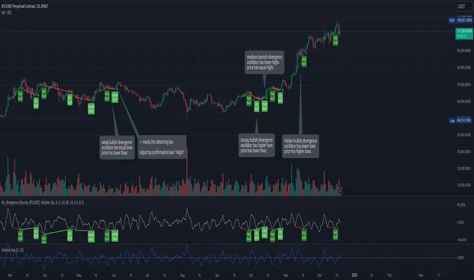
lib_divergenceLibrary "lib_divergence"
offers a commonly usable function to detect divergences. This will take the default RSI or other symbols / indicators / oscillators as source data.
divergence(osc, pivot_left_bars, pivot_right_bars, div_min_range, div_max_range, ref_low, ref_high, min_divergence_offset_fraction, min_divergence_offset_dev_len, min_divergence_offset_atr_mul)
Detects Divergences between Price and Oscillator action. For bullish divergences, look at trend lines between lows. For bearish divergences, look at trend lines between highs. (strong) oscillator trending, price opposing it | (medium) oscillator trending, price trend flat | (weak) price opposite trending, oscillator trend flat | (hidden) price trending, oscillator opposing it. Pivot detection is only properly done in oscillator data, reference price data is only compared at the oscillator pivot (speed optimization)
Parameters:
osc (float) : (series float) oscillator data (can be anything, even another instrument price)
pivot_left_bars (simple int) : (simple int) optional number of bars left of a confirmed pivot point, confirming it is the highest/lowest in the range before and up to the pivot (default: 5)
pivot_right_bars (simple int) : (simple int) optional number of bars right of a confirmed pivot point, confirming it is the highest/lowest in the range from and after the pivot (default: 5)
div_min_range (simple int) : (simple int) optional minimum distance to the pivot point creating a divergence (default: 5)
div_max_range (simple int) : (simple int) optional maximum amount of bars in a divergence (default: 50)
ref_low (float) : (series float) optional reference range to compare the oscillator pivot points to. (default: low)
ref_high (float) : (series float) optional reference range to compare the oscillator pivot points to. (default: high)
min_divergence_offset_fraction (simple float) : (simple float) optional scaling factor for the offset zone (xDeviation) around the last oscillator H/L detecting following equal H/Ls (default: 0.01)
min_divergence_offset_dev_len (simple int) : (simple int) optional lookback distance for the deviation detection for the offset zone around the last oscillator H/L detecting following equal H/Ls. Used as well for the ATR that does the equal H/L detection for the reference price. (default: 14)
min_divergence_offset_atr_mul (simple float) : (simple float) optional scaling factor for the offset zone (xATR) around the last price H/L detecting following equal H/Ls (default: 1)
@return A tuple of deviation flags.
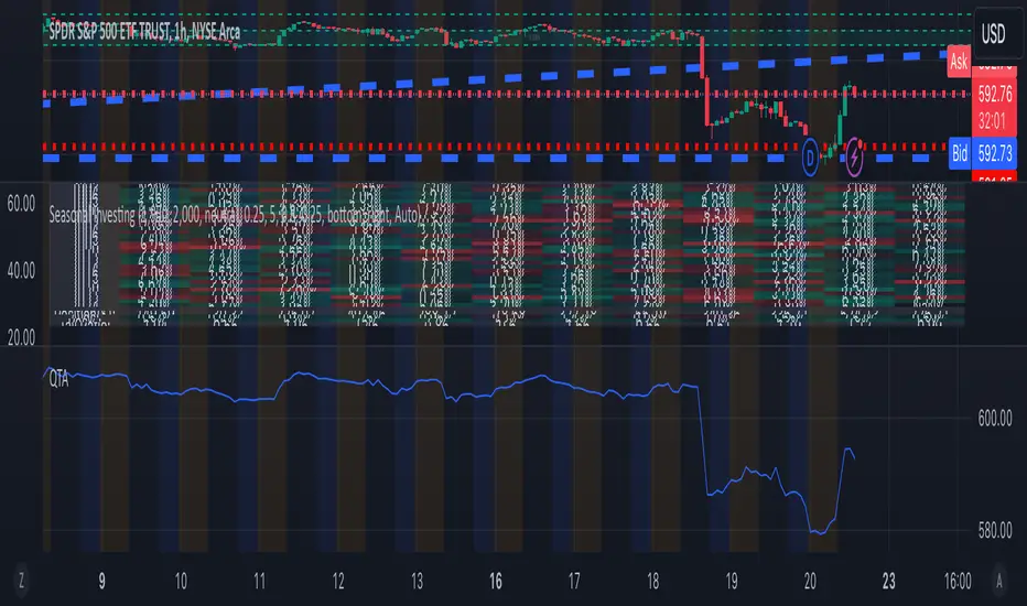
QTALibrary "QTA"
This is simple library for basic Quantitative Technical Analysis for retail investors. One example of it being used can be seen here ().
calculateKellyRatio(returns)
Parameters:
returns (array) : An array of floats representing the returns from bets.
Returns: The calculated Kelly Ratio, which indicates the optimal bet size based on winning and losing probabilities.
calculateAdjustedKellyFraction(kellyRatio, riskTolerance, fedStance)
Parameters:
kellyRatio (float) : The calculated Kelly Ratio.
riskTolerance (float) : A float representing the risk tolerance level.
fedStance (string) : A string indicating the Federal Reserve's stance ("dovish", "hawkish", or neutral).
Returns: The adjusted Kelly Fraction, constrained within the bounds of .
calculateStdDev(returns)
Parameters:
returns (array) : An array of floats representing the returns.
Returns: The standard deviation of the returns, or 0 if insufficient data.
calculateMaxDrawdown(returns)
Parameters:
returns (array) : An array of floats representing the returns.
Returns: The maximum drawdown as a percentage.
calculateEV(avgWinReturn, winProb, avgLossReturn)
Parameters:
avgWinReturn (float) : The average return from winning bets.
winProb (float) : The probability of winning a bet.
avgLossReturn (float) : The average return from losing bets.
Returns: The calculated Expected Value of the bet.
calculateTailRatio(returns)
Parameters:
returns (array) : An array of floats representing the returns.
Returns: The Tail Ratio, or na if the 5th percentile is zero to avoid division by zero.
calculateSharpeRatio(avgReturn, riskFreeRate, stdDev)
Parameters:
avgReturn (float) : The average return of the investment.
riskFreeRate (float) : The risk-free rate of return.
stdDev (float) : The standard deviation of the investment's returns.
Returns: The calculated Sharpe Ratio, or na if standard deviation is zero.
calculateDownsideDeviation(returns)
Parameters:
returns (array) : An array of floats representing the returns.
Returns: The standard deviation of the downside returns, or 0 if no downside returns exist.
calculateSortinoRatio(avgReturn, downsideDeviation)
Parameters:
avgReturn (float) : The average return of the investment.
downsideDeviation (float) : The standard deviation of the downside returns.
Returns: The calculated Sortino Ratio, or na if downside deviation is zero.
calculateVaR(returns, confidenceLevel)
Parameters:
returns (array) : An array of floats representing the returns.
confidenceLevel (float) : A float representing the confidence level (e.g., 0.95 for 95% confidence).
Returns: The Value at Risk at the specified confidence level.
calculateCVaR(returns, varValue)
Parameters:
returns (array) : An array of floats representing the returns.
varValue (float) : The Value at Risk threshold.
Returns: The average Conditional Value at Risk, or na if no returns are below the threshold.
calculateExpectedPriceRange(currentPrice, ev, stdDev, confidenceLevel)
Parameters:
currentPrice (float) : The current price of the asset.
ev (float) : The expected value (in percentage terms).
stdDev (float) : The standard deviation (in percentage terms).
confidenceLevel (float) : The confidence level for the price range (e.g., 1.96 for 95% confidence).
Returns: A tuple containing the minimum and maximum expected prices.
calculateRollingStdDev(returns, window)
Parameters:
returns (array) : An array of floats representing the returns.
window (int) : An integer representing the rolling window size.
Returns: An array of floats representing the rolling standard deviation of returns.
calculateRollingVariance(returns, window)
Parameters:
returns (array) : An array of floats representing the returns.
window (int) : An integer representing the rolling window size.
Returns: An array of floats representing the rolling variance of returns.
calculateRollingMean(returns, window)
Parameters:
returns (array) : An array of floats representing the returns.
window (int) : An integer representing the rolling window size.
Returns: An array of floats representing the rolling mean of returns.
calculateRollingCoefficientOfVariation(returns, window)
Parameters:
returns (array) : An array of floats representing the returns.
window (int) : An integer representing the rolling window size.
Returns: An array of floats representing the rolling coefficient of variation of returns.
calculateRollingSumOfPercentReturns(returns, window)
Parameters:
returns (array) : An array of floats representing the returns.
window (int) : An integer representing the rolling window size.
Returns: An array of floats representing the rolling sum of percent returns.
calculateRollingCumulativeProduct(returns, window)
Parameters:
returns (array) : An array of floats representing the returns.
window (int) : An integer representing the rolling window size.
Returns: An array of floats representing the rolling cumulative product of returns.
calculateRollingCorrelation(priceReturns, volumeReturns, window)
Parameters:
priceReturns (array) : An array of floats representing the price returns.
volumeReturns (array) : An array of floats representing the volume returns.
window (int) : An integer representing the rolling window size.
Returns: An array of floats representing the rolling correlation.
calculateRollingPercentile(returns, window, percentile)
Parameters:
returns (array) : An array of floats representing the returns.
window (int) : An integer representing the rolling window size.
percentile (int) : An integer representing the desired percentile (0-100).
Returns: An array of floats representing the rolling percentile of returns.
calculateRollingMaxMinPercentReturns(returns, window)
Parameters:
returns (array) : An array of floats representing the returns.
window (int) : An integer representing the rolling window size.
Returns: A tuple containing two arrays: rolling max and rolling min percent returns.
calculateRollingPriceToVolumeRatio(price, volData, window)
Parameters:
price (array) : An array of floats representing the price data.
volData (array) : An array of floats representing the volume data.
window (int) : An integer representing the rolling window size.
Returns: An array of floats representing the rolling price-to-volume ratio.
determineMarketRegime(priceChanges)
Parameters:
priceChanges (array) : An array of floats representing the price changes.
Returns: A string indicating the market regime ("Bull", "Bear", or "Neutral").
determineVolatilityRegime(price, window)
Parameters:
price (array) : An array of floats representing the price data.
window (int) : An integer representing the rolling window size.
Returns: An array of floats representing the calculated volatility.
classifyVolatilityRegime(volatility)
Parameters:
volatility (array) : An array of floats representing the calculated volatility.
Returns: A string indicating the volatility regime ("Low" or "High").
method percentPositive(thisArray)
Returns the percentage of positive non-na values in this array.
This method calculates the percentage of positive values in the provided array, ignoring NA values.
Namespace types: array
Parameters:
thisArray (array)
_candleRange()
_PreviousCandleRange(barsback)
Parameters:
barsback (int) : An integer representing how far back you want to get a range
redCandle()
greenCandle()
_WhiteBody()
_BlackBody()
HighOpenDiff()
OpenLowDiff()
_isCloseAbovePreviousOpen(length)
Parameters:
length (int)
_isCloseBelowPrevious()
_isOpenGreaterThanPrevious()
_isOpenLessThanPrevious()
BodyHigh()
BodyLow()
_candleBody()
_BodyAvg(length)
_BodyAvg function.
Parameters:
length (simple int) : Required (recommended is 6).
_SmallBody(length)
Parameters:
length (simple int) : Length of the slow EMA
Returns: a series of bools, after checking if the candle body was less than body average.
_LongBody(length)
Parameters:
length (simple int)
bearWick()
bearWick() function.
Returns: a SERIES of FLOATS, checks if it's a blackBody(open > close), if it is, than check the difference between the high and open, else checks the difference between high and close.
bullWick()
barlength()
sumbarlength()
sumbull()
sumbear()
bull_vol()
bear_vol()
volumeFightMA()
volumeFightDelta()
weightedAVG_BullVolume()
weightedAVG_BearVolume()
VolumeFightDiff()
VolumeFightFlatFilter()
avg_bull_vol(userMA)
avg_bull_vol(int) function.
Parameters:
userMA (int)
avg_bear_vol(userMA)
avg_bear_vol(int) function.
Parameters:
userMA (int)
diff_vol(userMA)
diff_vol(int) function.
Parameters:
userMA (int)
vol_flat(userMA)
vol_flat(int) function.
Parameters:
userMA (int)
_isEngulfingBullish()
_isEngulfingBearish()
dojiup()
dojidown()
EveningStar()
MorningStar()
ShootingStar()
Hammer()
InvertedHammer()
BearishHarami()
BullishHarami()
BullishBelt()
BullishKicker()
BearishKicker()
HangingMan()
DarkCloudCover()
CandleCandle: A Comprehensive Pine Script™ Library for Candlestick Analysis
Overview
The Candle library, developed in Pine Script™, provides traders and developers with a robust toolkit for analyzing candlestick data. By offering easy access to fundamental candlestick components like open, high, low, and close prices, along with advanced derived metrics such as body-to-wick ratios, percentage calculations, and volatility analysis, this library enables detailed insights into market behavior.
This library is ideal for creating custom indicators, trading strategies, and backtesting frameworks, making it a powerful resource for any Pine Script™ developer.
Key Features
1. Core Candlestick Data
• Open : Access the opening price of the current candle.
• High : Retrieve the highest price.
• Low : Retrieve the lowest price.
• Close : Access the closing price.
2. Candle Metrics
• Full Size : Calculates the total range of the candle (high - low).
• Body Size : Computes the size of the candle’s body (open - close).
• Wick Size : Provides the combined size of the upper and lower wicks.
3. Wick and Body Ratios
• Upper Wick Size and Lower Wick Size .
• Body-to-Wick Ratio and Wick-to-Body Ratio .
4. Percentage Calculations
• Upper Wick Percentage : The proportion of the upper wick size relative to the full candle size.
• Lower Wick Percentage : The proportion of the lower wick size relative to the full candle size.
• Body Percentage and Wick Percentage relative to the candle’s range.
5. Candle Direction Analysis
• Determines if a candle is "Bullish" or "Bearish" based on its closing and opening prices.
6. Price Metrics
• Average Price : The mean of the open, high, low, and close prices.
• Midpoint Price : The midpoint between the high and low prices.
7. Volatility Measurement
• Calculates the standard deviation of the OHLC prices, providing a volatility metric for the current candle.
Code Architecture
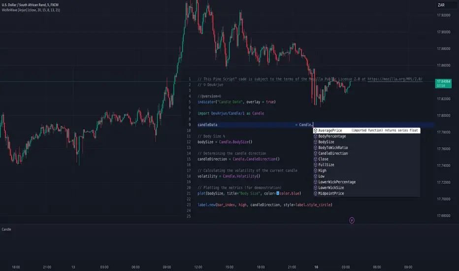
Example Functionality
The library employs a modular structure, exporting various functions that can be used independently or in combination. For instance:
// This Pine Script™ code is subject to the terms of the Mozilla Public License 2.0 at mozilla.org
// © DevArjun
//@version=6
indicator("Candle Data", overlay = true)
import DevArjun/Candle/1 as Candle
// Body Size %
bodySize = Candle.BodySize()
// Determining the candle direction
candleDirection = Candle.CandleDirection()
// Calculating the volatility of the current candle
volatility = Candle.Volatility()
// Plotting the metrics (for demonstration)
plot(bodySize, title="Body Size", color=color.blue)
label.new(bar_index, high, candleDirection, style=label.style_circle)
Scalability
The modularity of the Candle library allows seamless integration into more extensive trading systems. Functions can be mixed and matched to suit specific analytical or strategic needs.
Use Cases
Trading Strategies
Developers can use the library to create strategies based on candle properties such as:
• Identifying long-bodied candles (momentum signals).
• Detecting wicks as potential reversal zones.
• Filtering trades based on candle ratios.
Visualization
Plotting components like body size, wick size, and directional labels helps visualize market behavior and identify patterns.
Backtesting
By incorporating volatility and ratio metrics, traders can design and test strategies on historical data, ensuring robust performance before live trading.
Education
This library is a great tool for teaching candlestick analysis and how each component contributes to market behavior.
Portfolio Highlights
Project Objective
To create a Pine Script™ library that simplifies candlestick analysis by providing comprehensive metrics and insights, empowering traders and developers with advanced tools for market analysis.
Development Challenges and Solutions
• Challenge : Achieving high precision in calculating ratios and percentages.
• Solution : Implemented robust mathematical operations and safeguarded against division-by-zero errors.
• Challenge : Ensuring modularity and scalability.
• Solution : Designed functions as independent modules, allowing flexible integration.
Impact
• Efficiency : The library reduces the time required to calculate complex candlestick metrics.
• Versatility : Supports various trading styles, from scalping to swing trading.
• Clarity : Clean code and detailed documentation ensure usability for developers of all levels.
Conclusion
The Candle library exemplifies the power of Pine Script™ in simplifying and enhancing candlestick analysis. By including this project in your portfolio, you showcase your expertise in:
• Financial data analysis.
• Pine Script™ development.
• Creating tools that solve real-world trading challenges.
This project demonstrates both technical proficiency and a keen understanding of market analysis, making it an excellent addition to your professional portfolio.
Library "Candle"
A comprehensive library to access and analyze the basic components of a candlestick, including open, high, low, close prices, and various derived metrics such as full size, body size, wick sizes, ratios, percentages, and additional analysis metrics.
Open()
Open
@description Returns the opening price of the current candle.
Returns: float - The opening price of the current candle.
High()
High
@description Returns the highest price of the current candle.
Returns: float - The highest price of the current candle.
Low()
Low
@description Returns the lowest price of the current candle.
Returns: float - The lowest price of the current candle.
Close()
Close
@description Returns the closing price of the current candle.
Returns: float - The closing price of the current candle.
FullSize()
FullSize
@description Returns the full size (range) of the current candle (high - low).
Returns: float - The full size of the current candle.
BodySize()
BodySize
@description Returns the body size of the current candle (open - close).
Returns: float - The body size of the current candle.
WickSize()
WickSize
@description Returns the size of the wicks of the current candle (full size - body size).
Returns: float - The size of the wicks of the current candle.
UpperWickSize()
UpperWickSize
@description Returns the size of the upper wick of the current candle.
Returns: float - The size of the upper wick of the current candle.
LowerWickSize()
LowerWickSize
@description Returns the size of the lower wick of the current candle.
Returns: float - The size of the lower wick of the current candle.
BodyToWickRatio()
BodyToWickRatio
@description Returns the ratio of the body size to the wick size of the current candle.
Returns: float - The body to wick ratio of the current candle.
UpperWickPercentage()
UpperWickPercentage
@description Returns the percentage of the upper wick size relative to the full size of the current candle.
Returns: float - The percentage of the upper wick size relative to the full size of the current candle.
LowerWickPercentage()
LowerWickPercentage
@description Returns the percentage of the lower wick size relative to the full size of the current candle.
Returns: float - The percentage of the lower wick size relative to the full size of the current candle.
WickToBodyRatio()
WickToBodyRatio
@description Returns the ratio of the wick size to the body size of the current candle.
Returns: float - The wick to body ratio of the current candle.
BodyPercentage()
BodyPercentage
@description Returns the percentage of the body size relative to the full size of the current candle.
Returns: float - The percentage of the body size relative to the full size of the current candle.
WickPercentage()
WickPercentage
@description Returns the percentage of the wick size relative to the full size of the current candle.
Returns: float - The percentage of the wick size relative to the full size of the current candle.
CandleDirection()
CandleDirection
@description Returns the direction of the current candle.
Returns: string - "Bullish" if the candle is bullish, "Bearish" if the candle is bearish.
AveragePrice()
AveragePrice
@description Returns the average price of the current candle (mean of open, high, low, and close).
Returns: float - The average price of the current candle.
MidpointPrice()
MidpointPrice
@description Returns the midpoint price of the current candle (mean of high and low).
Returns: float - The midpoint price of the current candle.
Volatility()
Volatility
@description Returns the standard deviation of the OHLC prices of the current candle.
Returns: float - The volatility of the current candle.
DynamicPeriodPublicDynamic Period Calculation Library
This library provides tools for adaptive period determination, useful for creating indicators or strategies that automatically adjust to market conditions.
Overview
The Dynamic Period Library calculates adaptive periods based on pivot points, enabling the creation of responsive indicators and strategies that adjust to market volatility.
Key Features
Dynamic Periods: Computes periods using distances between pivot highs and lows.
Customizable Parameters: Users can adjust detection settings and period constraints.
Robust Handling: Includes fallback mechanisms for cases with insufficient pivot data.
Use Cases
Adaptive Indicators: Build tools that respond to market volatility by adjusting their periods dynamically.
Dynamic Strategies: Enhance trading strategies by integrating pivot-based period adjustments.
Function: `dynamic_period`
Description
Calculates a dynamic period based on the average distances between pivot highs and lows.
Parameters
`left` (default: 5): Number of left-hand bars for pivot detection.
`right` (default: 5): Number of right-hand bars for pivot detection.
`numPivots` (default: 5): Minimum pivots required for calculation.
`minPeriod` (default: 2): Minimum allowed period.
`maxPeriod` (default: 50): Maximum allowed period.
`defaultPeriod` (default: 14): Fallback period if no pivots are found.
Returns
A dynamic period calculated based on pivot distances, constrained by `minPeriod` and `maxPeriod`.
Example
//@version=6
import CrimsonVault/DynamicPeriodPublic/1
left = input.int(5, "Left bars", minval = 1)
right = input.int(5, "Right bars", minval = 1)
numPivots = input.int(5, "Number of Pivots", minval = 2)
period = DynamicPeriodPublic.dynamic_period(left, right, numPivots)
plot(period, title = "Dynamic Period", color = color.blue)
Implementation Notes
Pivot Detection: Requires sufficient historical data to identify pivots accurately.
Edge Cases: Ensures a default period is applied when pivots are insufficient.
Constraints: Limits period values to a user-defined range for stability.

lib_kernelLibrary "lib_kernel"
Library "lib_kernel"
This is a tool / library for developers, that contains several common and adapted kernel functions as well as a kernel regression function and enum to easily select and embed a list into the settings dialog.
How to Choose and Modify Kernels in Practice
Compact Support Kernels (e.g., Epanechnikov, Triangular): Use for localized smoothing and emphasizing nearby data.
Oscillatory Kernels (e.g., Wave, Cosine): Ideal for detecting periodic patterns or mean-reverting behavior.
Smooth Tapering Kernels (e.g., Gaussian, Logistic): Use for smoothing long-term trends or identifying global price behavior.
kernel_Epanechnikov(u)
Parameters:
u (float)
kernel_Epanechnikov_alt(u, sensitivity)
Parameters:
u (float)
sensitivity (float)
kernel_Triangular(u)
Parameters:
u (float)
kernel_Triangular_alt(u, sensitivity)
Parameters:
u (float)
sensitivity (float)
kernel_Rectangular(u)
Parameters:
u (float)
kernel_Uniform(u)
Parameters:
u (float)
kernel_Uniform_alt(u, sensitivity)
Parameters:
u (float)
sensitivity (float)
kernel_Logistic(u)
Parameters:
u (float)
kernel_Logistic_alt(u)
Parameters:
u (float)
kernel_Logistic_alt2(u, sigmoid_steepness)
Parameters:
u (float)
sigmoid_steepness (float)
kernel_Gaussian(u)
Parameters:
u (float)
kernel_Gaussian_alt(u, sensitivity)
Parameters:
u (float)
sensitivity (float)
kernel_Silverman(u)
Parameters:
u (float)
kernel_Quartic(u)
Parameters:
u (float)
kernel_Quartic_alt(u, sensitivity)
Parameters:
u (float)
sensitivity (float)
kernel_Biweight(u)
Parameters:
u (float)
kernel_Triweight(u)
Parameters:
u (float)
kernel_Sinc(u)
Parameters:
u (float)
kernel_Wave(u)
Parameters:
u (float)
kernel_Wave_alt(u)
Parameters:
u (float)
kernel_Cosine(u)
Parameters:
u (float)
kernel_Cosine_alt(u, sensitivity)
Parameters:
u (float)
sensitivity (float)
kernel(u, select, alt_modificator)
wrapper for all standard kernel functions, see enum Kernel comments and function descriptions for usage szenarios and parameters
Parameters:
u (float)
select (series Kernel)
alt_modificator (float)
kernel_regression(src, bandwidth, kernel, exponential_distance, alt_modificator)
wrapper for kernel regression with all standard kernel functions, see enum Kernel comments for usage szenarios. performance optimized version using fixed bandwidth and target
Parameters:
src (float) : input data series
bandwidth (simple int) : sample window of nearest neighbours for the kernel to process
kernel (simple Kernel) : type of Kernel to use for processing, see Kernel enum or respective functions for more details
exponential_distance (simple bool) : if true this puts more emphasis on local / more recent values
alt_modificator (float) : see kernel functions for parameter descriptions. Mostly used to pronounce emphasis on local values or introduce a decay/dampening to the kernel output

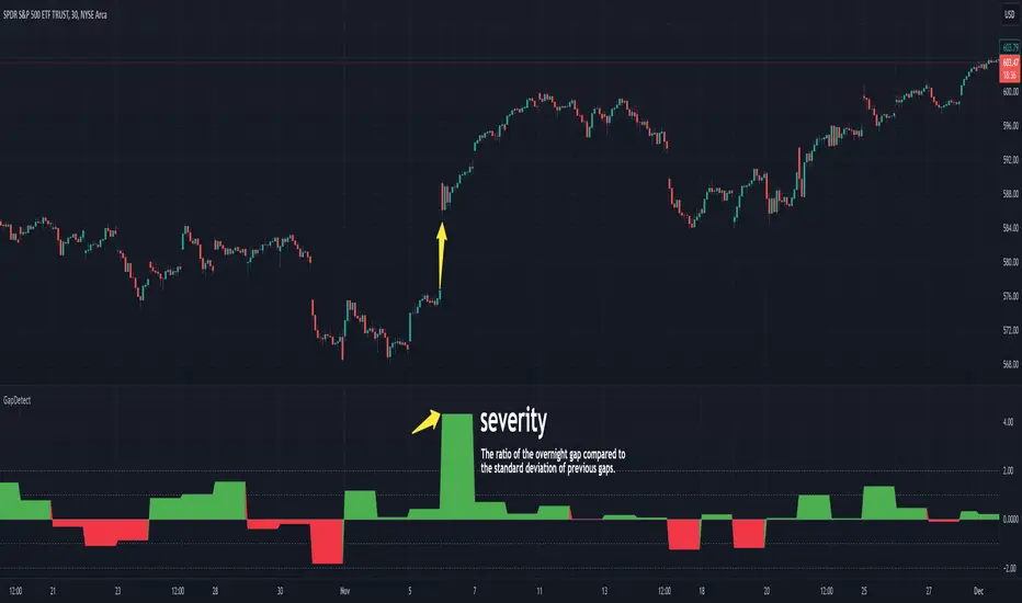
GapDetectGap Severity Analysis Library
This library, GapDetect , simplifies the identification and evaluation of overnight gaps by leveraging statistical metrics such as standard deviation and percentage moves. It is ideal for detecting large abnormal gaps which may be used to modify how strategies may decide to enter or exit.
Key Features:
Overnight Gap Detection
Provides two core functions:
today : Computes the value of today's overnight gap.
todayPercent : Computes the percentage change for today's overnight gap.
Volatility Analysis
Includes functions for statistical gap analysis:
normal : Calculates the normal daily standard deviation of the overnight gap, filtering outliers using customizable thresholds.
normalPercent : Similar to normal , but for percentage-based gap moves.
Gap Severity Metric
severity : a positive or negative value that represents the ratio of the current overnight move compared to the standard deviation of previous ones.
Customizable Parameters
Supports custom session specifications, resolutions, and outlier thresholds.
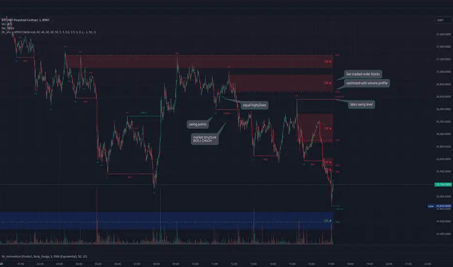
lib_smcLibrary "lib_smc"
This is an adaptation of LuxAlgo's Smart Money Concepts indicator with numerous changes. Main changes include integration of object based plotting, plenty of performance improvements, live tracking of Order Blocks, integration of volume profiles to refine Order Blocks, and many more.
This is a library for developers, if you want this converted into a working strategy, let me know.
buffer(item, len, force_rotate)
Parameters:
item (float)
len (int)
force_rotate (bool)
buffer(item, len, force_rotate)
Parameters:
item (int)
len (int)
force_rotate (bool)
buffer(item, len, force_rotate)
Parameters:
item (Profile type from robbatt/lib_profile/32)
len (int)
force_rotate (bool)
swings(len)
INTERNAL: detect swing points (HH and LL) in given range
Parameters:
len (simple int) : range to check for new swing points
Returns: values are the price level where and if a new HH or LL was detected, else na
method init(this)
Namespace types: OrderBlockConfig
Parameters:
this (OrderBlockConfig)
method delete(this)
Namespace types: OrderBlock
Parameters:
this (OrderBlock)
method clear_broken(this, broken_buffer)
INTERNAL: delete internal order blocks box coordinates if top/bottom is broken
Namespace types: map
Parameters:
this (map)
broken_buffer (map)
Returns: any_bull_ob_broken, any_bear_ob_broken, broken signals are true if an according order block was broken/mitigated, broken contains the broken block(s)
create_ob(id, mode, start_t, start_i, top, end_t, end_i, bottom, break_price, early_confirmation_price, config, init_plot, force_overlay)
INTERNAL: set internal order block coordinates
Parameters:
id (int)
mode (int) : 1: bullish, -1 bearish block
start_t (int)
start_i (int)
top (float)
end_t (int)
end_i (int)
bottom (float)
break_price (float)
early_confirmation_price (float)
config (OrderBlockConfig)
init_plot (bool)
force_overlay (bool)
Returns: signals are true if an according order block was broken/mitigated
method align_to_profile(block, align_edge, align_break_price)
Namespace types: OrderBlock
Parameters:
block (OrderBlock)
align_edge (bool)
align_break_price (bool)
method create_profile(block, opens, tops, bottoms, closes, values, resolution, vah_pc, val_pc, args, init_calculated, init_plot, force_overlay)
Namespace types: OrderBlock
Parameters:
block (OrderBlock)
opens (array)
tops (array)
bottoms (array)
closes (array)
values (array)
resolution (int)
vah_pc (float)
val_pc (float)
args (ProfileArgs type from robbatt/lib_profile/32)
init_calculated (bool)
init_plot (bool)
force_overlay (bool)
method create_profile(block, resolution, vah_pc, val_pc, args, init_calculated, init_plot, force_overlay)
Namespace types: OrderBlock
Parameters:
block (OrderBlock)
resolution (int)
vah_pc (float)
val_pc (float)
args (ProfileArgs type from robbatt/lib_profile/32)
init_calculated (bool)
init_plot (bool)
force_overlay (bool)
track_obs(swing_len, hh, ll, top, btm, bull_bos_alert, bull_choch_alert, bear_bos_alert, bear_choch_alert, min_block_size, max_block_size, config_bull, config_bear, init_plot, force_overlay, enabled, extend_blocks, clear_broken_buffer_before, align_edge_to_value_area, align_break_price_to_poc, profile_args_bull, profile_args_bear, use_soft_confirm, soft_confirm_offset, use_retracements_with_FVG_out)
Parameters:
swing_len (int)
hh (float)
ll (float)
top (float)
btm (float)
bull_bos_alert (bool)
bull_choch_alert (bool)
bear_bos_alert (bool)
bear_choch_alert (bool)
min_block_size (float)
max_block_size (float)
config_bull (OrderBlockConfig)
config_bear (OrderBlockConfig)
init_plot (bool)
force_overlay (bool)
enabled (bool)
extend_blocks (simple bool)
clear_broken_buffer_before (simple bool)
align_edge_to_value_area (simple bool)
align_break_price_to_poc (simple bool)
profile_args_bull (ProfileArgs type from robbatt/lib_profile/32)
profile_args_bear (ProfileArgs type from robbatt/lib_profile/32)
use_soft_confirm (simple bool)
soft_confirm_offset (float)
use_retracements_with_FVG_out (simple bool)
method draw(this, config, extend_only)
Namespace types: OrderBlock
Parameters:
this (OrderBlock)
config (OrderBlockConfig)
extend_only (bool)
method draw(blocks, config)
INTERNAL: plot order blocks
Namespace types: array
Parameters:
blocks (array)
config (OrderBlockConfig)
method draw(blocks, config)
INTERNAL: plot order blocks
Namespace types: map
Parameters:
blocks (map)
config (OrderBlockConfig)
method cleanup(this, ob_bull, ob_bear)
removes all Profiles that are older than the latest OrderBlock from this profile buffer
Namespace types: array
Parameters:
this (array type from robbatt/lib_profile/32)
ob_bull (OrderBlock)
ob_bear (OrderBlock)
_plot_swing_points(mode, x, y, show_swing_points, linecolor_swings, keep_history, show_latest_swings_levels, trail_x, trail_y, trend)
INTERNAL: plot swing points
Parameters:
mode (int) : 1: bullish, -1 bearish block
x (int) : x-coordingate of swing point to plot (bar_index)
y (float) : y-coordingate of swing point to plot (price)
show_swing_points (bool) : switch to enable/disable plotting of swing point labels
linecolor_swings (color) : color for swing point labels and lates level lines
keep_history (bool) : weater to remove older swing point labels and only keep the most recent
show_latest_swings_levels (bool)
trail_x (int) : x-coordinate for latest swing point (bar_index)
trail_y (float) : y-coordinate for latest swing point (price)
trend (int) : the current trend 1: bullish, -1: bearish, to determine Strong/Weak Low/Highs
_pivot_lvl(mode, trend, hhll_x, hhll, super_hhll, filter_insignificant_internal_breaks)
INTERNAL: detect whether a structural level has been broken and if it was in trend direction (BoS) or against trend direction (ChoCh), also track the latest high and low swing points
Parameters:
mode (simple int) : detect 1: bullish, -1 bearish pivot points
trend (int) : current trend direction
hhll_x (int) : x-coordinate of newly detected hh/ll (bar_index)
hhll (float) : y-coordinate of newly detected hh/ll (price)
super_hhll (float) : level/y-coordinate of superior hhll (if this is an internal structure pivot level)
filter_insignificant_internal_breaks (bool) : if true pivot points / internal structure will be ignored where the wick in trend direction is longer than the opposite (likely to push further in direction of main trend)
Returns: coordinates of internal structure that has been broken (x,y): start of structure, (trail_x, trail_y): tracking hh/ll after structure break, (bos_alert, choch_alert): signal whether a structural level has been broken
_plot_structure(x, y, is_bos, is_choch, line_color, line_style, label_style, label_size, keep_history)
INTERNAL: plot structural breaks (BoS/ChoCh)
Parameters:
x (int) : x-coordinate of newly broken structure (bar_index)
y (float) : y-coordinate of newly broken structure (price)
is_bos (bool) : whether this structural break was in trend direction
is_choch (bool) : whether this structural break was against trend direction
line_color (color) : color for the line connecting the structural level and the breaking candle
line_style (string) : style (line.style_dashed/solid) for the line connecting the structural level and the breaking candle
label_style (string) : style (label.style_label_down/up) for the label above/below the line connecting the structural level and the breaking candle
label_size (string) : size (size.small/tiny) for the label above/below the line connecting the structural level and the breaking candle
keep_history (bool) : weater to remove older swing point labels and only keep the most recent
structure_values(length, super_hh, super_ll, filter_insignificant_internal_breaks)
detect (and plot) structural breaks and the resulting new trend
Parameters:
length (simple int) : lookback period for swing point detection
super_hh (float) : level/y-coordinate of superior hh (for internal structure detection)
super_ll (float) : level/y-coordinate of superior ll (for internal structure detection)
filter_insignificant_internal_breaks (bool) : if true pivot points / internal structure will be ignored where the wick in trend direction is longer than the opposite (likely to push further in direction of main trend)
Returns: trend: direction 1:bullish -1:bearish, (bull_bos_alert, bull_choch_alert, top_x, top_y, trail_up_x, trail_up): whether and which level broke in a bullish direction, trailing high, (bbear_bos_alert, bear_choch_alert, tm_x, btm_y, trail_dn_x, trail_dn): same in bearish direction
structure_plot(trend, bull_bos_alert, bull_choch_alert, top_x, top_y, trail_up_x, trail_up, hh, bear_bos_alert, bear_choch_alert, btm_x, btm_y, trail_dn_x, trail_dn, ll, color_bull, color_bear, show_swing_points, show_latest_swings_levels, show_bos, show_choch, line_style, label_size, keep_history)
detect (and plot) structural breaks and the resulting new trend
Parameters:
trend (int) : crrent trend 1: bullish, -1: bearish
bull_bos_alert (bool) : if there was a bullish bos alert -> plot it
bull_choch_alert (bool) : if there was a bullish choch alert -> plot it
top_x (int) : latest shwing high x
top_y (float) : latest swing high y
trail_up_x (int) : trailing high x
trail_up (float) : trailing high y
hh (float) : if there was a higher high
bear_bos_alert (bool) : if there was a bearish bos alert -> plot it
bear_choch_alert (bool) : if there was a bearish chock alert -> plot it
btm_x (int) : latest swing low x
btm_y (float) : latest swing low y
trail_dn_x (int) : trailing low x
trail_dn (float) : trailing low y
ll (float) : if there was a lower low
color_bull (color) : color for bullish BoS/ChoCh levels
color_bear (color) : color for bearish BoS/ChoCh levels
show_swing_points (bool) : whether to plot swing point labels
show_latest_swings_levels (bool) : whether to track and plot latest swing point levels with lines
show_bos (bool) : whether to plot BoS levels
show_choch (bool) : whether to plot ChoCh levels
line_style (string) : whether to plot BoS levels
label_size (string) : label size of plotted BoS/ChoCh levels
keep_history (bool) : weater to remove older swing point labels and only keep the most recent
structure(length, color_bull, color_bear, super_hh, super_ll, filter_insignificant_internal_breaks, show_swing_points, show_latest_swings_levels, show_bos, show_choch, line_style, label_size, keep_history, enabled)
detect (and plot) structural breaks and the resulting new trend
Parameters:
length (simple int) : lookback period for swing point detection
color_bull (color) : color for bullish BoS/ChoCh levels
color_bear (color) : color for bearish BoS/ChoCh levels
super_hh (float) : level/y-coordinate of superior hh (for internal structure detection)
super_ll (float) : level/y-coordinate of superior ll (for internal structure detection)
filter_insignificant_internal_breaks (bool) : if true pivot points / internal structure will be ignored where the wick in trend direction is longer than the opposite (likely to push further in direction of main trend)
show_swing_points (bool) : whether to plot swing point labels
show_latest_swings_levels (bool) : whether to track and plot latest swing point levels with lines
show_bos (bool) : whether to plot BoS levels
show_choch (bool) : whether to plot ChoCh levels
line_style (string) : whether to plot BoS levels
label_size (string) : label size of plotted BoS/ChoCh levels
keep_history (bool) : weater to remove older swing point labels and only keep the most recent
enabled (bool)
_check_equal_level(mode, len, eq_threshold, enabled)
INTERNAL: detect equal levels (double top/bottom)
Parameters:
mode (int) : detect 1: bullish/high, -1 bearish/low pivot points
len (int) : lookback period for equal level (swing point) detection
eq_threshold (float) : maximum price offset for a level to be considered equal
enabled (bool)
Returns: eq_alert whether an equal level was detected and coordinates of the first and the second level/swing point
_plot_equal_level(show_eq, x1, y1, x2, y2, label_txt, label_style, label_size, line_color, line_style, keep_history)
INTERNAL: plot equal levels (double top/bottom)
Parameters:
show_eq (bool) : whether to plot the level or not
x1 (int) : x-coordinate of the first level / swing point
y1 (float) : y-coordinate of the first level / swing point
x2 (int) : x-coordinate of the second level / swing point
y2 (float) : y-coordinate of the second level / swing point
label_txt (string) : text for the label above/below the line connecting the equal levels
label_style (string) : style (label.style_label_down/up) for the label above/below the line connecting the equal levels
label_size (string) : size (size.tiny) for the label above/below the line connecting the equal levels
line_color (color) : color for the line connecting the equal levels (and it's label)
line_style (string) : style (line.style_dotted) for the line connecting the equal levels
keep_history (bool) : weater to remove older swing point labels and only keep the most recent
equal_levels_values(len, threshold, enabled)
detect (and plot) equal levels (double top/bottom), returns coordinates
Parameters:
len (int) : lookback period for equal level (swing point) detection
threshold (float) : maximum price offset for a level to be considered equal
enabled (bool) : whether detection is enabled
Returns: (eqh_alert, eqh_x1, eqh_y1, eqh_x2, eqh_y2) whether an equal high was detected and coordinates of the first and the second level/swing point, (eql_alert, eql_x1, eql_y1, eql_x2, eql_y2) same for equal lows
equal_levels_plot(eqh_x1, eqh_y1, eqh_x2, eqh_y2, eql_x1, eql_y1, eql_x2, eql_y2, color_eqh, color_eql, show, keep_history)
detect (and plot) equal levels (double top/bottom), returns coordinates
Parameters:
eqh_x1 (int) : coordinates of first point of equal high
eqh_y1 (float) : coordinates of first point of equal high
eqh_x2 (int) : coordinates of second point of equal high
eqh_y2 (float) : coordinates of second point of equal high
eql_x1 (int) : coordinates of first point of equal low
eql_y1 (float) : coordinates of first point of equal low
eql_x2 (int) : coordinates of second point of equal low
eql_y2 (float) : coordinates of second point of equal low
color_eqh (color) : color for the line connecting the equal highs (and it's label)
color_eql (color) : color for the line connecting the equal lows (and it's label)
show (bool) : whether plotting is enabled
keep_history (bool) : weater to remove older swing point labels and only keep the most recent
Returns: (eqh_alert, eqh_x1, eqh_y1, eqh_x2, eqh_y2) whether an equal high was detected and coordinates of the first and the second level/swing point, (eql_alert, eql_x1, eql_y1, eql_x2, eql_y2) same for equal lows
equal_levels(len, threshold, color_eqh, color_eql, enabled, show, keep_history)
detect (and plot) equal levels (double top/bottom)
Parameters:
len (int) : lookback period for equal level (swing point) detection
threshold (float) : maximum price offset for a level to be considered equal
color_eqh (color) : color for the line connecting the equal highs (and it's label)
color_eql (color) : color for the line connecting the equal lows (and it's label)
enabled (bool) : whether detection is enabled
show (bool) : whether plotting is enabled
keep_history (bool) : weater to remove older swing point labels and only keep the most recent
Returns: (eqh_alert) whether an equal high was detected, (eql_alert) same for equal lows
_detect_fvg(mode, enabled, o, h, l, c, filter_insignificant_fvgs, change_tf)
INTERNAL: detect FVG (fair value gap)
Parameters:
mode (int) : detect 1: bullish, -1 bearish gaps
enabled (bool) : whether detection is enabled
o (float) : reference source open
h (float) : reference source high
l (float) : reference source low
c (float) : reference source close
filter_insignificant_fvgs (bool) : whether to calculate and filter small/insignificant gaps
change_tf (bool) : signal when the previous reference timeframe closed, triggers new calculation
Returns: whether a new FVG was detected and its top/mid/bottom levels
_clear_broken_fvg(mode, upper_boxes, lower_boxes)
INTERNAL: clear mitigated FVGs (fair value gaps)
Parameters:
mode (int) : detect 1: bullish, -1 bearish gaps
upper_boxes (array) : array that stores the upper parts of the FVG boxes
lower_boxes (array) : array that stores the lower parts of the FVG boxes
_plot_fvg(mode, show, top, mid, btm, border_color, extend_box)
INTERNAL: plot (and clear broken) FVG (fair value gap)
Parameters:
mode (int) : plot 1: bullish, -1 bearish gap
show (bool) : whether plotting is enabled
top (float) : top level of fvg
mid (float) : center level of fvg
btm (float) : bottom level of fvg
border_color (color) : color for the FVG box
extend_box (int) : how many bars into the future the FVG box should be extended after detection
fvgs_values(o, h, l, c, filter_insignificant_fvgs, change_tf, enabled)
detect (and plot / clear broken) FVGs (fair value gaps), and return alerts and level values
Parameters:
o (float) : reference source open
h (float) : reference source high
l (float) : reference source low
c (float) : reference source close
filter_insignificant_fvgs (bool) : whether to calculate and filter small/insignificant gaps
change_tf (bool) : signal when the previous reference timeframe closed, triggers new calculation
enabled (bool) : whether detection is enabled
Returns: (bullish_fvg_alert, bull_top, bull_mid, bull_btm): whether a new bullish FVG was detected and its top/mid/bottom levels, (bearish_fvg_alert, bear_top, bear_mid, bear_btm): same for bearish FVGs
fvgs_plot(bullish_fvg_alert, bull_top, bull_mid, bull_btm, bearish_fvg_alert, bear_top, bear_mid, bear_btm, color_bull, color_bear, extend_box, show)
Parameters:
bullish_fvg_alert (bool)
bull_top (float)
bull_mid (float)
bull_btm (float)
bearish_fvg_alert (bool)
bear_top (float)
bear_mid (float)
bear_btm (float)
color_bull (color) : color for bullish FVG boxes
color_bear (color) : color for bearish FVG boxes
extend_box (int) : how many bars into the future the FVG box should be extended after detection
show (bool) : whether plotting is enabled
Returns: (bullish_fvg_alert, bull_top, bull_mid, bull_btm): whether a new bullish FVG was detected and its top/mid/bottom levels, (bearish_fvg_alert, bear_top, bear_mid, bear_btm): same for bearish FVGs
fvgs(o, h, l, c, filter_insignificant_fvgs, change_tf, color_bull, color_bear, extend_box, enabled, show)
detect (and plot / clear broken) FVGs (fair value gaps)
Parameters:
o (float) : reference source open
h (float) : reference source high
l (float) : reference source low
c (float) : reference source close
filter_insignificant_fvgs (bool) : whether to calculate and filter small/insignificant gaps
change_tf (bool) : signal when the previous reference timeframe closed, triggers new calculation
color_bull (color) : color for bullish FVG boxes
color_bear (color) : color for bearish FVG boxes
extend_box (int) : how many bars into the future the FVG box should be extended after detection
enabled (bool) : whether detection is enabled
show (bool) : whether plotting is enabled
Returns: (bullish_fvg_alert): whether a new bullish FVG was detected, (bearish_fvg_alert): same for bearish FVGs
OrderBlock
Fields:
id (series int)
dir (series int)
left_top (chart.point)
right_bottom (chart.point)
break_price (series float)
early_confirmation_price (series float)
ltf_high (array)
ltf_low (array)
ltf_volume (array)
plot (Box type from robbatt/lib_plot_objects/49)
profile (Profile type from robbatt/lib_profile/32)
trailing (series bool)
extending (series bool)
awaiting_confirmation (series bool)
touched_break_price_before_confirmation (series bool)
soft_confirmed (series bool)
has_fvg_out (series bool)
hidden (series bool)
broken (series bool)
OrderBlockConfig
Fields:
show (series bool)
show_last (series int)
show_id (series bool)
show_profile (series bool)
args (BoxArgs type from robbatt/lib_plot_objects/49)
txt (series string)
txt_args (BoxTextArgs type from robbatt/lib_plot_objects/49)
delete_when_broken (series bool)
broken_args (BoxArgs type from robbatt/lib_plot_objects/49)
broken_txt (series string)
broken_txt_args (BoxTextArgs type from robbatt/lib_plot_objects/49)
broken_profile_args (ProfileArgs type from robbatt/lib_profile/32)
use_profile (series bool)
profile_args (ProfileArgs type from robbatt/lib_profile/32)
BacktestLibraryLibrary "BacktestLibrary"
A library providing functions for equity calculation and performance metrics.
since(date, active)
: Calculates the number of candles since a specified date.
Parameters:
date (simple float) : (simple float): The starting date in timestamp format (e.g., input.time(timestamp()))
active (simple bool) : (simple bool): If true, counts the number of candles since the date; if false, returns 0.
Returns: (int): The number of candles since the specified date.
buy_and_hold(r, startDate)
: Calculates the Buy and Hold Equity from a specified date.
Parameters:
r (float) : (series float): Daily returns of the asset (e.g., 0.02 for 2% move).
startDate (simple float) : (simple float): Timestamp of the starting date for the equity calculation.
Returns: (float): Buy and Hold Equity of the asset from the specified date.
equity(sig, threshold, r, startDate, signals)
: Calculates the strategy's equity on a candle-by-candle basis.
Parameters:
sig (float) : (series float): Signal values; positive for long, negative for short.
threshold (simple float) : (simple float): Signal threshold for entering trades.
r (float) : (series float): Daily returns of the asset (e.g., 0.02 for 2% move).
startDate (simple float) : (simple float): Timestamp of the starting date for the equity calculation.
signals (simple string) : (simple string): Type of signals to backtest ("Long & Short", "Long Only", "Short Only").
Returns: (float): Strategy equity on a candle-by-candle basis.
PerformanceMetrics(base, Lookback, startDate)
: Calculates performance metrics of a strategy from a specified date.
Parameters:
base (float) : (series float): Equity values of the strategy or Buy and Hold equity.
Lookback (int) : (series int): Number of periods since the start date; recommended to use the 'since' function.
startDate (simple float) : (simple float): Timestamp of the starting date for the equity calculation.
Returns: (float ): Array of performance metrics.
PerfMetricTable(buy_and_hold, strategy)
: Plots a table comparing performance metrics of Buy and Hold and Strategy equity.
Parameters:
buy_and_hold (array) : (float ): Metrics from the PerformanceMetrics() function for Buy and Hold.
strategy (array) : (float ): Metrics from the PerformanceMetrics() function for the strategy.
Returns: : Table displaying the performance metrics comparison.

ArrayMovingAveragesLibrary "ArrayMovingAverages"
This library adds several moving average methods to arrays, so you can call, eg.:
myArray.ema(3)
method emaArray(id, length)
Calculate Exponential Moving Average (EMA) for Arrays
Namespace types: array
Parameters:
id (array) : (array) Input array
length (int) : (int) Length of the EMA
Returns: (array) Array of EMA values
method ema(id, length)
Get the last value of the EMA array
Namespace types: array
Parameters:
id (array) : (array) Input array
length (int) : (int) Length of the EMA
Returns: (float) Last EMA value or na if empty
method rmaArray(id, length)
Calculate Rolling Moving Average (RMA) for Arrays
Namespace types: array
Parameters:
id (array) : (array) Input array
length (int) : (int) Length of the RMA
Returns: (array) Array of RMA values
method rma(id, length)
Get the last value of the RMA array
Namespace types: array
Parameters:
id (array) : (array) Input array
length (int) : (int) Length of the RMA
Returns: (float) Last RMA value or na if empty
method smaArray(id, windowSize)
Calculate Simple Moving Average (SMA) for Arrays
Namespace types: array
Parameters:
id (array) : (array) Input array
windowSize (int) : (int) Window size for calculation, defaults to array size
Returns: (array) Array of SMA values
method sma(id, windowSize)
Get the last value of the SMA array
Namespace types: array
Parameters:
id (array) : (array) Input array
windowSize (int) : (int) Window size for calculation, defaults to array size
Returns: (float) Last SMA value or na if empty
method wmaArray(id, windowSize)
Calculate Weighted Moving Average (WMA) for Arrays
Namespace types: array
Parameters:
id (array) : (array) Input array
windowSize (int) : (int) Window size for calculation, defaults to array size
Returns: (array) Array of WMA values
method wma(id, windowSize)
Get the last value of the WMA array
Namespace types: array
Parameters:
id (array) : (array) Input array
windowSize (int) : (int) Window size for calculation, defaults to array size
Returns: (float) Last WMA value or na if empty

QuantifyPS - 1Library "QuantifyPS"
normdist(z)
Parameters:
z (float) : (float): The z-score for which the CDF is to be calculated.
Returns: (float): The cumulative probability corresponding to the input z-score.
Notes:
- Uses an approximation method for the normal distribution CDF, which is computationally efficient.
- The result is accurate for most practical purposes but may have minor deviations for extreme values of `z`.
Formula:
- Based on the approximation formula:
`Φ(z) ≈ 1 - f(z) * P(t)` if `z > 0`, otherwise `Φ(z) ≈ f(z) * P(t)`,
where:
`f(z) = 0.3989423 * exp(-z^2 / 2)` (PDF of standard normal distribution)
`P(t) = Σ [c * t^i]` with constants `c` and `t = 1 / (1 + 0.2316419 * |z|)`.
Implementation details:
- The approximation uses five coefficients for the polynomial part of the CDF.
- Handles both positive and negative values of `z` symmetrically.
Constants:
- The coefficients and scaling factors are chosen to minimize approximation errors.
gamma(x)
Parameters:
x (float) : (float): The input value for which the Gamma function is to be calculated.
Must be greater than 0. For x <= 0, the function returns `na` as it is undefined.
Returns: (float): Approximation of the Gamma function for the input `x`.
Notes:
- The Lanczos approximation provides a numerically stable and efficient method to compute the Gamma function.
- The function is not defined for `x <= 0` and will return `na` in such cases.
- Uses precomputed Lanczos coefficients for accuracy.
- Includes handling for small numerical inaccuracies.
Formula:
- The Gamma function is approximated as:
`Γ(x) ≈ sqrt(2π) * t^(x + 0.5) * e^(-t) * Σ(p / (x + k))`
where `t = x + g + 0.5` and `p` is the array of Lanczos coefficients.
Implementation details:
- Lanczos coefficients (`p`) are precomputed and stored in an array.
- The summation iterates over these coefficients to compute the final result.
- The constant `g` controls the precision of the approximation (commonly `g = 7`).
t_cdf(t, df)
Parameters:
t (float) : (float): The t-statistic for which the CDF value is to be calculated.
df (int) : (int): Degrees of freedom of the t-distribution.
Returns: (float): Approximate CDF value for the given t-statistic.
Notes:
- This function computes a one-tailed p-value.
- Relies on an approximation formula using gamma functions and standard t-distribution properties.
- May not be as accurate as specialized statistical libraries for extreme values or very high degrees of freedom.
Formula:
- Let `x = df / (t^2 + df)`.
- The approximation formula is derived using:
`CDF(t, df) ≈ 1 - * x^((df + 1) / 2) / 2`,
where Γ represents the gamma function.
Implementation details:
- Computes the gamma ratio for normalization.
- Applies the t-distribution formula for one-tailed probabilities.
tStatForPValue(p, df)
Parameters:
p (float) : (float): P-value for which the t-statistic needs to be calculated.
Must be in the interval (0, 1).
df (int) : (int): Degrees of freedom of the t-distribution.
Returns: (float): The t-statistic corresponding to the given p-value.
Notes:
- If `p` is outside the interval (0, 1), the function returns `na` as an error.
- The function uses binary search with a fixed number of iterations and a defined tolerance.
- The result is accurate to within the specified tolerance (default: 0.0001).
- Relies on the cumulative density function (CDF) `t_cdf` for the t-distribution.
Formula:
- Uses the cumulative density function (CDF) of the t-distribution to iteratively find the t-statistic.
Implementation details:
- `low` and `high` define the search interval for the t-statistic.
- The midpoint (`mid`) is iteratively refined until the difference between the cumulative probability
and the target p-value is smaller than the tolerance.
jarqueBera(n, s, k)
Parameters:
n (float) : (series float): Number of observations in the dataset.
s (float) : (series float): Skewness of the dataset.
k (float) : (series float): Kurtosis of the dataset.
Returns: (float): The Jarque-Bera test statistic.
Formula:
JB = n *
Notes:
- A higher JB value suggests that the data deviates more from a normal distribution.
- The test is asymptotically distributed as a chi-squared distribution with 2 degrees of freedom.
- Use this value to calculate a p-value to determine the significance of the result.
skewness(data)
Parameters:
data (float) : (series float): Input data series.
Returns: (float): The skewness value.
Notes:
- Handles missing values (`na`) by ignoring invalid points.
- Includes error handling for zero variance to avoid division-by-zero scenarios.
- Skewness is calculated as the normalized third central moment of the data.
kurtosis(data)
Parameters:
data (float) : (series float): Input data series.
Returns: (float): The kurtosis value.
Notes:
- Handles missing values (`na`) by ignoring invalid points.
- Includes error handling for zero variance to avoid division-by-zero scenarios.
- Kurtosis is calculated as the normalized fourth central moment of the data.
regression(y, x, lag)
Parameters:
y (float) : (series float): Dependent series (observed values).
x (float) : (series float): Independent series (explanatory variable).
lag (int) : (int): Number of lags applied to the independent series (x).
Returns: (tuple): Returns a tuple containing the following values:
- n: Number of valid observations.
- alpha: Intercept of the regression line.
- beta: Slope of the regression line.
- t_stat: T-statistic for the beta coefficient.
- p_value: Two-tailed p-value for the beta coefficient.
- r_squared: Coefficient of determination (R²) indicating goodness of fit.
- skew: Skewness of the residuals.
- kurt: Kurtosis of the residuals.
Notes:
- Handles missing data (`na`) by ignoring invalid points.
- Includes basic error handling for zero variance and division-by-zero scenarios.
- Computes residual-based statistics (skewness and kurtosis) for model diagnostics.
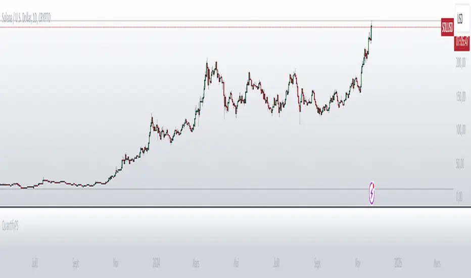
GaussianDistributionLibrary "GaussianDistribution"
This library defines a custom type `distr` representing a Gaussian (or other statistical) distribution.
It provides methods to calculate key statistical moments and scores, including mean, median, mode, standard deviation, variance, skewness, kurtosis, and Z-scores.
This library is useful for analyzing probability distributions in financial data.
Disclaimer:
I am not a mathematician, but I have implemented this library to the best of my understanding and capacity. Please be indulgent as I tried to translate statistical concepts into code as accurately as possible. Feedback, suggestions, and corrections are welcome to improve the reliability and robustness of this library.
mean(source, length)
Calculate the mean (average) of the distribution
Parameters:
source (float) : Distribution source (typically a price or indicator series)
length (int) : Window length for the distribution (must be >= 30 for meaningful statistics)
Returns: Mean (μ)
stdev(source, length)
Calculate the standard deviation (σ) of the distribution
Parameters:
source (float) : Distribution source (typically a price or indicator series)
length (int) : Window length for the distribution (must be >= 30 for meaningful statistics)
Returns: Standard deviation (σ)
skewness(source, length, mean, stdev)
Calculate the skewness (γ₁) of the distribution
Parameters:
source (float) : Distribution source (typically a price or indicator series)
length (int) : Window length for the distribution (must be >= 30 for meaningful statistics)
mean (float) : the mean (average) of the distribution
stdev (float) : the standard deviation (σ) of the distribution
@return Skewness (γ₁)
skewness(source, length)
Overloaded skewness to calculate from source and length
Parameters:
source (float) : Distribution source (typically a price or indicator series)
length (int) : Window length for the distribution (must be >= 30 for meaningful statistics)
@return Skewness (γ₁)
mode(mean, stdev, skewness)
Estimate mode - Most frequent value in the distribution (approximation based on skewness)
Parameters:
mean (float) : the mean (average) of the distribution
stdev (float) : the standard deviation (σ) of the distribution
skewness (float) : the skewness (γ₁) of the distribution
@return Mode
mode(source, length)
Overloaded mode to calculate from source and length
Parameters:
source (float) : Distribution source (typically a price or indicator series)
length (int) : Window length for the distribution (must be >= 30 for meaningful statistics)
@return Mode
median(mean, stdev, skewness)
Estimate median - Middle value of the distribution (approximation)
Parameters:
mean (float) : the mean (average) of the distribution
stdev (float) : the standard deviation (σ) of the distribution
skewness (float) : the skewness (γ₁) of the distribution
@return Median
median(source, length)
Overloaded median to calculate from source and length
Parameters:
source (float) : Distribution source (typically a price or indicator series)
length (int) : Window length for the distribution (must be >= 30 for meaningful statistics)
@return Median
variance(stdev)
Calculate variance (σ²) - Square of the standard deviation
Parameters:
stdev (float) : the standard deviation (σ) of the distribution
@return Variance (σ²)
variance(source, length)
Overloaded variance to calculate from source and length
Parameters:
source (float) : Distribution source (typically a price or indicator series)
length (int) : Window length for the distribution (must be >= 30 for meaningful statistics)
@return Variance (σ²)
kurtosis(source, length, mean, stdev)
Calculate kurtosis (γ₂) - Degree of "tailedness" in the distribution
Parameters:
source (float) : Distribution source (typically a price or indicator series)
length (int) : Window length for the distribution (must be >= 30 for meaningful statistics)
mean (float) : the mean (average) of the distribution
stdev (float) : the standard deviation (σ) of the distribution
@return Kurtosis (γ₂)
kurtosis(source, length)
Overloaded kurtosis to calculate from source and length
Parameters:
source (float) : Distribution source (typically a price or indicator series)
length (int) : Window length for the distribution (must be >= 30 for meaningful statistics)
@return Kurtosis (γ₂)
normal_score(source, mean, stdev)
Calculate Z-score (standard score) assuming a normal distribution
Parameters:
source (float) : Distribution source (typically a price or indicator series)
mean (float) : the mean (average) of the distribution
stdev (float) : the standard deviation (σ) of the distribution
@return Z-Score
normal_score(source, length)
Overloaded normal_score to calculate from source and length
Parameters:
source (float) : Distribution source (typically a price or indicator series)
length (int) : Window length for the distribution (must be >= 30 for meaningful statistics)
@return Z-Score
non_normal_score(source, mean, stdev, skewness, kurtosis)
Calculate adjusted Z-score considering skewness and kurtosis
Parameters:
source (float) : Distribution source (typically a price or indicator series)
mean (float) : the mean (average) of the distribution
stdev (float) : the standard deviation (σ) of the distribution
skewness (float) : the skewness (γ₁) of the distribution
kurtosis (float) : the "tailedness" in the distribution
@return Z-Score
non_normal_score(source, length)
Overloaded non_normal_score to calculate from source and length
Parameters:
source (float) : Distribution source (typically a price or indicator series)
length (int) : Window length for the distribution (must be >= 30 for meaningful statistics)
@return Z-Score
method init(this)
Initialize all statistical fields of the `distr` type
Namespace types: distr
Parameters:
this (distr)
method init(this, source, length)
Overloaded initializer to set source and length
Namespace types: distr
Parameters:
this (distr)
source (float)
length (int)
distr
Custom type to represent a Gaussian distribution
Fields:
source (series float) : Distribution source (typically a price or indicator series)
length (series int) : Window length for the distribution (must be >= 30 for meaningful statistics)
mode (series float) : Most frequent value in the distribution
median (series float) : Middle value separating the greater and lesser halves of the distribution
mean (series float) : μ (1st central moment) - Average of the distribution
stdev (series float) : σ or standard deviation (square root of the variance) - Measure of dispersion
variance (series float) : σ² (2nd central moment) - Squared standard deviation
skewness (series float) : γ₁ (3rd central moment) - Asymmetry of the distribution
kurtosis (series float) : γ₂ (4th central moment) - Degree of "tailedness" relative to a normal distribution
normal_score (series float) : Z-score assuming normal distribution
non_normal_score (series float) : Adjusted Z-score considering skewness and kurtosis
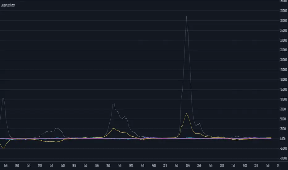
MathHelpersLibrary "MathHelpers"
Overview
A collection of helper functions for designing indicators and strategies.
calculateATR(length, log)
Calculates the Average True Range (ATR) or Log ATR based on the 'log' parameter. Sans Wilder's Smoothing
Parameters:
length (simple int)
log (simple bool)
Returns: float The calculated ATR value. Returns Log ATR if `log` is true, otherwise returns standard ATR.
CDF(z)
Computes the Cumulative Distribution Function (CDF) for a given value 'z', mimicking the CDF function in "Statistically Sound Indicators" by Timothy Masters.
Parameters:
z (simple float)
Returns: float The CDF value corresponding to the input `z`, ranging between 0 and 1.
logReturns(lookback)
Calculates the logarithmic returns over a specified lookback period.
Parameters:
lookback (simple int)
Returns: float The calculated logarithmic return. Returns `na` if insufficient data is available.
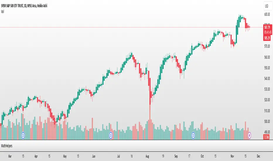
RHR_CANDLELibrary "RHR_CANDLE"
Library for Expansion Contraction Indicator, a zero-lag dual perspective indicator based on Jake Bernstein’s principles of Moving Average Channel system.
calc(shortLookback, longLookback)
Calculates Expansion Contraction values.
Parameters:
shortLookback (int) : Integer for the short lookback calculation, defaults to 8
longLookback (int) : Integer for the long lookback calculation, defaults to 32
@return Returns array of Expansion Contraction values
stdevCalc(positiveShort, negativeShort, positiveLong, negativeLong, stdevLookback)
Calculates standard deviation lines based on Expansion Contraction Long and Short values.
Parameters:
positiveShort (float) : Float for the positive short XC value from calculation
negativeShort (float) : Float for the negative short XC value from calculation
positiveLong (float) : Float for the positive long XC value from calculation
negativeLong (float) : Float for the negative long XC value from calculation
stdevLookback (int) : Integer for the standard deviation lookback, defaults to 500
@return Returns array of standard deviation values
trend(positiveShort, negativeShort, positiveLong, negativeLong)
Determines if trend is strong or weak based on Expansion Contraction values.
Parameters:
positiveShort (float) : Float for the positive short XC value from calculation
negativeShort (float) : Float for the negative short XC value from calculation
positiveLong (float) : Float for the positive long XC value from calculation
negativeLong (float) : Float for the negative long XC value from calculation
@return Returns array of boolean values indicating strength or weakness of trend

lib_momentumLibrary "lib_momentum"
This library calculates the momentum, derived from a sample range of prior candles. Depending on set MomentumType it either deduces the momentum from the price, volume, or a product of both. If price/product are selected, you can choose from SampleType if only candle body, full range from high to low or a combination of both (body counts full, wicks half for each direction) should be used. Optional: You can choose to normalize the results, dividing each value by its average (normalization_ma_length, normalization_ma). This will allow comparison between different instruments. For the normalization Moving Average you can choose any currently supported in my lib_no_delay.
get_momentum(momentum_type, sample_type, sample_length, normalization_ma_length, normalization_ma)
Parameters:
momentum_type (series MomentumType) : select one of MomentumType. to sample the price, volume or a product of both
sample_type (series SampleType) : select one of SampleType. to sample the body, total range from high to low or a combination of both (body count full, wicks half for each direction)
sample_length (simple int) : how many candles should be sampled (including the current)
normalization_ma_length (simple int) : if you want to normalize results (momentum / momentum average) this sets the period for the average. (default = 0 => no normalization)
normalization_ma (simple MovingAverage enum from robbatt/lib_no_delay/9) : is the type of moving average to normalize / compare with
Returns: returns the current momentum where the total line is not just (up - down) but also sampled over the sample_length and can therefore be used as trend indicator. If up/down fail to reach total's level it's a sign of decreasing momentum, if up/down exceed total the trend it's a sign of increasing momentum.
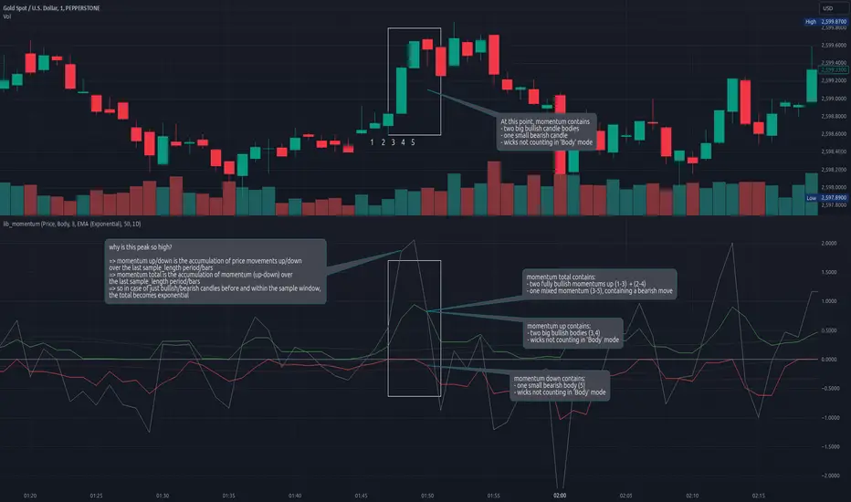
PRINT_DROVINGLibrary "PRINT_DROVING"
method print_droving(foot_bar, sup)
printing all footprint objects
Namespace types: footprint_type.Footprint_bar
Parameters:
foot_bar (Footprint_bar type from Alesetup/PRINT_TYPE/1) : instance of Footprint_bar type
sup (Support_objects type from Alesetup/PRINT_TYPE/1) : instance of Support_objects type
Returns: Void.

PRINT_LOGICLibrary "PRINT_LOGIC"
method fill_imba_line(imba_line, foot_bar, sup)
fill imbalance line
Namespace types: footprint_type.Imbalance_line
Parameters:
imba_line (Imbalance_line type from Alesetup/PRINT_TYPE/1) : instance of Imbalance_line type
foot_bar (Footprint_bar type from Alesetup/PRINT_TYPE/1) : instance of Footprint_bar type
sup (Support_objects type from Alesetup/PRINT_TYPE/1) : instance of Support_objects type
Returns: Void
method fill_footprint_type(foot_bar, sup)
Namespace types: footprint_type.Footprint_bar
Parameters:
foot_bar (Footprint_bar type from Alesetup/PRINT_TYPE/1) : instance of Footprint_bar type
sup (Support_objects type from Alesetup/PRINT_TYPE/1) : instance of Support_objects type
Returns: Void
method fill_footprint_object(foot_bar, sup)
fill all footprint objects
Namespace types: footprint_type.Footprint_bar
Parameters:
foot_bar (Footprint_bar type from Alesetup/PRINT_TYPE/1) : instance of Footprint_bar type
sup (Support_objects type from Alesetup/PRINT_TYPE/1) : instance of Support_objects type
Returns: Void
PRINT_TYPELibrary "PRINT_TYPE"
Inputs
Inputs objects
Fields:
inbalance_percent (series int) : percentage coefficient to determine the Imbalance of price levels
stacked_input (series int) : minimum number of consecutive Imbalance levels required to draw extended lines
show_summary_footprint (series bool)
procent_volume_area (series int) : definition size Value area
new_imbalance_cond (series bool) : bool input for setup alert on new imbalance buy and sell
new_imbalance_line_cond (series bool) : bool input for setup alert on new imbalance line buy and sell
stop_past_imbalance_line_cond (series bool) : bool input for setup alert on stop past imbalance line buy and sell
Constants
Constants all Constants objects
Fields:
imbalance_high_char (series string) : char for printing buy imbalance
imbalance_low_char (series string) : char for printing sell imbalance
color_title_sell (series color) : color for footprint sell
color_title_buy (series color) : color for footprint buy
color_line_sell (series color) : color for sell line
color_line_buy (series color) : color for buy line
color_title_none (series color) : color None
Calculation_data
Calculation_data data for calculating
Fields:
detail_open (array) : array open from calculation timeframe
detail_high (array) : array high from calculation timeframe
detail_low (array) : array low from calculation timeframe
detail_close (array) : array close from calculation timeframe
detail_vol (array) : array volume from calculation timeframe
previos_detail_close (array) : array close from calculation timeframe
isBuyVolume (series bool) : attribute previosly bar buy or sell
Footprint_row
Footprint_row objects one footprint row
Fields:
price (series float) : row price
buy_vol (series float) : buy volume
sell_vol (series float) : sell volume
imbalance_buy (series bool) : attribute buy inbalance
imbalance_sell (series bool) : attribute sell imbalance
buy_vol_box (series box) : for ptinting buy volume
sell_vol_box (series box) : for printing sell volume
buy_vp_box (series box) : for ptinting volume profile buy
sell_vp_box (series box) : for ptinting volume profile sell
row_line (series label) : for ptinting row price
empty (series bool) : = true attribute row with zero volume buy and zero volume sell
Imbalance_line_var_object
Imbalance_line_var_object var objects printing and calculation imbalance line
Fields:
cum_buy_line (array) : line array for saving all history buy imbalance line
cum_sell_line (array) : line array for saving all history sell imbalance line
Imbalance_line
Imbalance_line objects printing and calculation imbalance line
Fields:
buy_price_line (array) : float array for saving buy imbalance price level
sell_price_line (array) : float array for saving sell imbalance price level
var_imba_line (Imbalance_line_var_object) : var objects this type
Footprint_bar
Footprint_bar all objects one bar with footprint
Fields:
foot_rows (array) : objects one row footprint
imba_line (Imbalance_line) : objects imbalance line
row_size (series float) : size rows
total_vol (series float) : total volume one footprint bar
foot_buy_vol (series float) : buy volume one footprint bar
foot_sell_vol (series float) : sell volume one footprint bar
foot_max_price_vol (map) : map with one value - price row with max volume buy + sell
calc_data (Calculation_data) : objects with detail data from calculation resolution
Support_objects
Support_objects support object for footprint calculation
Fields:
consts (Constants) : all consts objects
inp (Inputs) : all input objects
bar_index_show_condition (series bool) : calculation bool value for show all objects footprint
row_line_color (series color) : calculation value - color for row price
dop_info (series string)
show_table_cond (series bool)
analytics_tablesLibrary "analytics_tables"
📝 Description
This library provides the implementation of several performance-related statistics and metrics, presented in the form of tables.
The metrics shown in the afforementioned tables where developed during the past years of my in-depth analalysis of various strategies in an atempt to reason about the performance of each strategy.
The visualization and some statistics where inspired by the existing implementations of the "Seasonality" script, and the performance matrix implementations of @QuantNomad and @ZenAndTheArtOfTrading scripts.
While this library is meant to be used by my strategy framework "Template Trailing Strategy (Backtester)" script, I wrapped it in a library hoping this can be usefull for other community strategy scripts that will be released in the future.
🤔 How to Guide
To use the functionality this library provides in your script you have to import it first!
Copy the import statement of the latest release by pressing the copy button below and then paste it into your script. Give a short name to this library so you can refer to it later on. The import statement should look like this:
import jason5480/analytics_tables/1 as ant
There are three types of tables provided by this library in the initial release. The stats table the metrics table and the seasonality table.
Each one shows different kinds of performance statistics.
The table UDT shall be initialized once using the `init()` method.
They can be updated using the `update()` method where the updated data UDT object shall be passed.
The data UDT can also initialized and get updated on demend depending on the use case
A code example for the StatsTable is the following:
var ant.StatsData statsData = ant.StatsData.new()
statsData.update(SideStats.new(), SideStats.new(), 0)
if (barstate.islastconfirmedhistory or (barstate.isrealtime and barstate.isconfirmed))
var statsTable = ant.StatsTable.new().init(ant.getTablePos('TOP', 'RIGHT'))
statsTable.update(statsData)
A code example for the MetricsTable is the following:
var ant.StatsData statsData = ant.StatsData.new()
statsData.update(ant.SideStats.new(), ant.SideStats.new(), 0)
if (barstate.islastconfirmedhistory or (barstate.isrealtime and barstate.isconfirmed))
var metricsTable = ant.MetricsTable.new().init(ant.getTablePos('BOTTOM', 'RIGHT'))
metricsTable.update(statsData, 10)
A code example for the SeasonalityTable is the following:
var ant.SeasonalData seasonalData = ant.SeasonalData.new().init(Seasonality.monthOfYear)
seasonalData.update()
if (barstate.islastconfirmedhistory or (barstate.isrealtime and barstate.isconfirmed))
var seasonalTable = ant.SeasonalTable.new().init(seasonalData, ant.getTablePos('BOTTOM', 'LEFT'))
seasonalTable.update(seasonalData)
🏋️♂️ Please refer to the "EXAMPLE" regions of the script for more advanced and up to date code examples!
Special thanks to @Mrcrbw for the proposal to develop this library and @DCNeu for the constructive feedback 🏆.
getTablePos(ypos, xpos)
Get table position compatible string
Parameters:
ypos (simple string) : The position on y axise
xpos (simple string) : The position on x axise
Returns: The position to be passed to the table
method init(this, pos, height, width, positiveTxtColor, negativeTxtColor, neutralTxtColor, positiveBgColor, negativeBgColor, neutralBgColor)
Initialize the stats table object with the given colors in the given position
Namespace types: StatsTable
Parameters:
this (StatsTable) : The stats table object
pos (simple string) : The table position string
height (simple float) : The height of the table as a percentage of the charts height. By default, 0 auto-adjusts the height based on the text inside the cells
width (simple float) : The width of the table as a percentage of the charts height. By default, 0 auto-adjusts the width based on the text inside the cells
positiveTxtColor (simple color) : The text color when positive
negativeTxtColor (simple color) : The text color when negative
neutralTxtColor (simple color) : The text color when neutral
positiveBgColor (simple color) : The background color with transparency when positive
negativeBgColor (simple color) : The background color with transparency when negative
neutralBgColor (simple color) : The background color with transparency when neutral
method init(this, pos, height, width, neutralBgColor)
Initialize the metrics table object with the given colors in the given position
Namespace types: MetricsTable
Parameters:
this (MetricsTable) : The metrics table object
pos (simple string) : The table position string
height (simple float) : The height of the table as a percentage of the charts height. By default, 0 auto-adjusts the height based on the text inside the cells
width (simple float) : The width of the table as a percentage of the charts width. By default, 0 auto-adjusts the width based on the text inside the cells
neutralBgColor (simple color) : The background color with transparency when neutral
method init(this, seas)
Initialize the seasonal data
Namespace types: SeasonalData
Parameters:
this (SeasonalData) : The seasonal data object
seas (simple Seasonality) : The seasonality of the matrix data
method init(this, data, pos, maxNumOfYears, height, width, extended, neutralTxtColor, neutralBgColor)
Initialize the seasonal table object with the given colors in the given position
Namespace types: SeasonalTable
Parameters:
this (SeasonalTable) : The seasonal table object
data (SeasonalData) : The seasonality data of the table
pos (simple string) : The table position string
maxNumOfYears (simple int) : The maximum number of years that fit into the table
height (simple float) : The height of the table as a percentage of the charts height. By default, 0 auto-adjusts the height based on the text inside the cells
width (simple float) : The width of the table as a percentage of the charts width. By default, 0 auto-adjusts the width based on the text inside the cells
extended (simple bool) : The seasonal table with extended columns for performance
neutralTxtColor (simple color) : The text color when neutral
neutralBgColor (simple color) : The background color with transparency when neutral
method update(this, wins, losses, numOfInconclusiveExits)
Update the strategy info data of the strategy
Namespace types: StatsData
Parameters:
this (StatsData) : The strategy statistics object
wins (SideStats)
losses (SideStats)
numOfInconclusiveExits (int) : The number of inconclusive trades
method update(this, stats, positiveTxtColor, negativeTxtColor, negativeBgColor, neutralBgColor)
Update the stats table object with the given data
Namespace types: StatsTable
Parameters:
this (StatsTable) : The stats table object
stats (StatsData) : The stats data to update the table
positiveTxtColor (simple color) : The text color when positive
negativeTxtColor (simple color) : The text color when negative
negativeBgColor (simple color) : The background color with transparency when negative
neutralBgColor (simple color) : The background color with transparency when neutral
method update(this, stats, buyAndHoldPerc, positiveTxtColor, negativeTxtColor, positiveBgColor, negativeBgColor)
Update the metrics table object with the given data
Namespace types: MetricsTable
Parameters:
this (MetricsTable) : The metrics table object
stats (StatsData) : The stats data to update the table
buyAndHoldPerc (float) : The buy and hold percetage
positiveTxtColor (simple color) : The text color when positive
negativeTxtColor (simple color) : The text color when negative
positiveBgColor (simple color) : The background color with transparency when positive
negativeBgColor (simple color) : The background color with transparency when negative
method update(this)
Update the seasonal data based on the season and eon timeframe
Namespace types: SeasonalData
Parameters:
this (SeasonalData) : The seasonal data object
method update(this, data, positiveTxtColor, negativeTxtColor, neutralTxtColor, positiveBgColor, negativeBgColor, neutralBgColor, timeBgColor)
Update the seasonal table object with the given data
Namespace types: SeasonalTable
Parameters:
this (SeasonalTable) : The seasonal table object
data (SeasonalData) : The seasonal cell data to update the table
positiveTxtColor (simple color) : The text color when positive
negativeTxtColor (simple color) : The text color when negative
neutralTxtColor (simple color) : The text color when neutral
positiveBgColor (simple color) : The background color with transparency when positive
negativeBgColor (simple color) : The background color with transparency when negative
neutralBgColor (simple color) : The background color with transparency when neutral
timeBgColor (simple color) : The background color of the time gradient
SideStats
Object that represents the strategy statistics data of one side win or lose
Fields:
numOf (series int)
sumFreeProfit (series float)
freeProfitStDev (series float)
sumProfit (series float)
profitStDev (series float)
sumGain (series float)
gainStDev (series float)
avgQuantityPerc (series float)
avgCapitalRiskPerc (series float)
avgTPExecutedCount (series float)
avgRiskRewardRatio (series float)
maxStreak (series int)
StatsTable
Object that represents the stats table
Fields:
table (series table) : The actual table
rows (series int) : The number of rows of the table
columns (series int) : The number of columns of the table
StatsData
Object that represents the statistics data of the strategy
Fields:
wins (SideStats)
losses (SideStats)
numOfInconclusiveExits (series int)
avgFreeProfitStr (series string)
freeProfitStDevStr (series string)
lossFreeProfitStDevStr (series string)
avgProfitStr (series string)
profitStDevStr (series string)
lossProfitStDevStr (series string)
avgQuantityStr (series string)
MetricsTable
Object that represents the metrics table
Fields:
table (series table) : The actual table
rows (series int) : The number of rows of the table
columns (series int) : The number of columns of the table
SeasonalData
Object that represents the seasonal table dynamic data
Fields:
seasonality (series Seasonality)
eonToMatrixRow (map)
numOfEons (series int)
mostRecentMatrixRow (series int)
balances (matrix)
returnPercs (matrix)
maxDDs (matrix)
eonReturnPercs (array)
eonCAGRs (array)
eonMaxDDs (array)
SeasonalTable
Object that represents the seasonal table
Fields:
table (series table) : The actual table
headRows (series int) : The number of head rows of the table
headColumns (series int) : The number of head columns of the table
eonRows (series int) : The number of eon rows of the table
seasonColumns (series int) : The number of season columns of the table
statsRows (series int)
statsColumns (series int) : The number of stats columns of the table
rows (series int) : The number of rows of the table
columns (series int) : The number of columns of the table
extended (series bool) : Whether the table has additional performance statistics

[ALGOA+] Markov Chains Library by @metacamaleoLibrary "MarkovChains"
Markov Chains library by @metacamaleo. Created in 09/08/2024.
This library provides tools to calculate and visualize Markov Chain-based transition matrices and probabilities. This library supports two primary algorithms: a rolling window Markov Chain and a conditional Markov Chain (which operates based on specified conditions). The key concepts used include Markov Chain states, transition matrices, and future state probabilities based on past market conditions or indicators.
Key functions:
- `mc_rw()`: Builds a transition matrix using a rolling window Markov Chain, calculating probabilities based on a fixed length of historical data.
- `mc_cond()`: Builds a conditional Markov Chain transition matrix, calculating probabilities based on the current market condition or indicator state.
Basically, you will just need to use the above functions on your script to default outputs and displays.
Exported UDTs include:
- s_map: An UDT variable used to store a map with dummy states, i.e., if possible states are bullish, bearish, and neutral, and current is bullish, it will be stored
in a map with following keys and values: "bullish", 1; "bearish", 0; and "neutral", 0. You will only use it to customize your own script, otherwise, it´s only for internal use.
- mc_states: This UDT variable stores user inputs, calculations and MC outputs. As the above, you don´t need to use it, but you may get features to customize your own script.
For example, you may use mc.tm to get the transition matrix, or the prob map to customize the display. As you see, functions are all based on mc_states UDT. The s_map UDT is used within mc_states´s s array.
Optional exported functions include:
- `mc_table()`: Displays the transition matrix in a table format on the chart for easy visualization of the probabilities.
- `display_list()`: Displays a map (or array) of string and float/int values in a table format, used for showing transition counts or probabilities.
- `mc_prob()`: Calculates and displays probabilities for a given number of future bars based on the current state in the Markov Chain.
- `mc_all_states_prob()`: Calculates probabilities for all states for future bars, considering all possible transitions.
The above functions may be used to customize your outputs. Use the returned variable mc_states from mc_rw() and mc_cond() to display each of its matrix, maps or arrays using mc_table() (for matrices) and display_list() (for maps and arrays) if you desire to debug or track the calculation process.
See the examples in the end of this script.
Have good trading days!
Best regards,
@metacamaleo
-----------------------------
KEY FUNCTIONS
mc_rw(state, length, states, pred_length, show_table, show_prob, table_position, prob_position, font_size)
Builds the transition matrix for a rolling window Markov Chain.
Parameters:
state (string) : The current state of the market or system.
length (int) : The rolling window size.
states (array) : Array of strings representing the possible states in the Markov Chain.
pred_length (int) : The number of bars to predict into the future.
show_table (bool) : Boolean to show or hide the transition matrix table.
show_prob (bool) : Boolean to show or hide the probability table.
table_position (string) : Position of the transition matrix table on the chart.
prob_position (string) : Position of the probability list on the chart.
font_size (string) : Size of the table font.
Returns: The transition matrix and probabilities for future states.
mc_cond(state, condition, states, pred_length, show_table, show_prob, table_position, prob_position, font_size)
Builds the transition matrix for conditional Markov Chains.
Parameters:
state (string) : The current state of the market or system.
condition (string) : A string representing the condition.
states (array) : Array of strings representing the possible states in the Markov Chain.
pred_length (int) : The number of bars to predict into the future.
show_table (bool) : Boolean to show or hide the transition matrix table.
show_prob (bool) : Boolean to show or hide the probability table.
table_position (string) : Position of the transition matrix table on the chart.
prob_position (string) : Position of the probability list on the chart.
font_size (string) : Size of the table font.
Returns: The transition matrix and probabilities for future states based on the HMM.
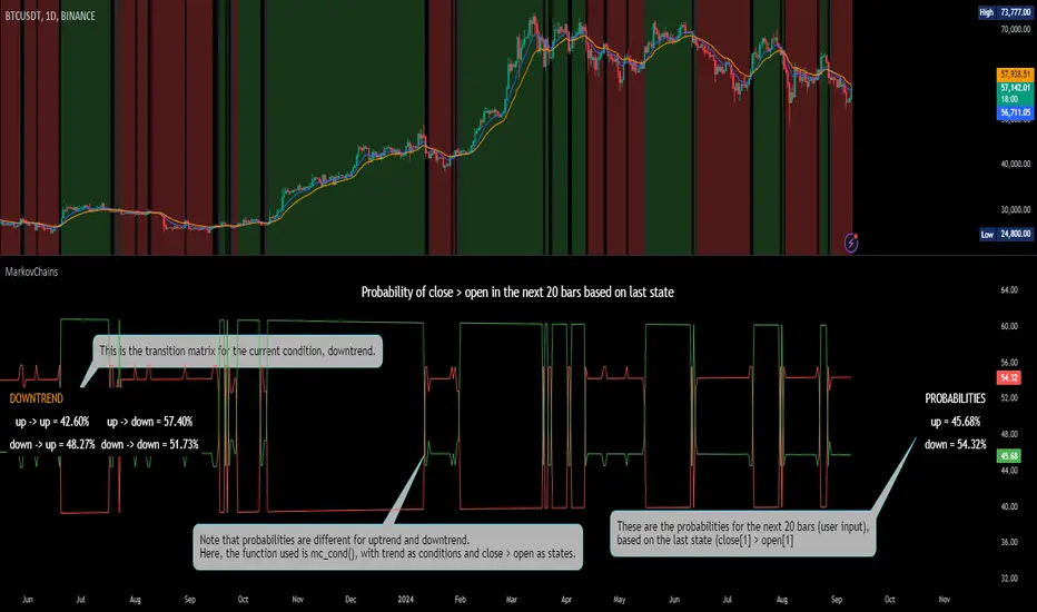
lib_no_delayLibrary "lib_no_delay"
This library contains modifications to standard functions that return na before reaching the bar of their 'length' parameter.
That is because they do not compromise speed at current time for correct results in the past. This is good for live trading in short timeframes but killing applications on Monthly / Weekly timeframes if instruments, like in crypto, do not have extensive history (why would you even trade the monthly on a meme coin ... not my decision).
Also, some functions rely on source (value at previous bar), which is not available on bar 1 and therefore cascading to a na value up to the last bar ... which in turn leads to a non displaying indicator and waste of time debugging this)
Anyway ... there you go, let me know if I should add more functions.
sma(source, length)
Parameters:
source (float) : Series of values to process.
length (simple int) : Number of bars (length).
Returns: Simple moving average of source for length bars back.
ema(source, length)
Parameters:
source (float) : Series of values to process.
length (simple int) : Number of bars (length).
Returns: (float) The exponentially weighted moving average of the source.
rma(source, length)
Parameters:
source (float) : Series of values to process.
length (simple int) : Number of bars (length).
Returns: Exponential moving average of source with alpha = 1 / length.
atr(length)
Function atr (average true range) returns the RMA of true range. True range is max(high - low, abs(high - close ), abs(low - close )). This adapted version extends ta.atr to start without delay at first bar and deliver usable data instead of na by averaging ta.tr(true) via manual SMA.
Parameters:
length (simple int) : Number of bars back (length).
Returns: Average true range.
rsi(source, length)
Relative strength index. It is calculated using the ta.rma() of upward and downward changes of source over the last length bars. This adapted version extends ta.rsi to start without delay at first bar and deliver usable data instead of na.
Parameters:
source (float) : Series of values to process.
length (simple int) : Number of bars back (length).
Returns: Relative Strength Index.

GraphLibrary "Graph"
Library to collect data and draw scatterplot and heatmap as graph
method init(this)
Initialise Quadrant Data
Namespace types: Quadrant
Parameters:
this (Quadrant) : Quadrant object that needs to be initialised
Returns: current Quadrant object
method init(this)
Initialise Graph Data
Namespace types: Graph
Parameters:
this (Graph) : Graph object that needs to be initialised with 4 Quadrants
Returns: current Graph object
method add(this, data)
Add coordinates to graph
Namespace types: Graph
Parameters:
this (Graph) : Graph object
data (Coordinate) : Coordinates containing x, y data
Returns: current Graph object
method calculate(this)
Calculation required for plotting the graph
Namespace types: Graph
Parameters:
this (Graph) : Graph object
Returns: current Graph object
method paint(this)
Draw graph
Namespace types: Graph
Parameters:
this (Graph) : Graph object
Returns: current Graph object
Coordinate
Coordinates of sample data
Fields:
xValue (series float) : x value of the sample data
yValue (series float) : y value of the sample data
Quadrant
Data belonging to particular quadrant
Fields:
coordinates (array) : Coordinates present in given quadrant
GraphProperties
Properties of Graph that needs to be drawn
Fields:
rows (series int) : Number of rows (y values) in each quadrant
columns (series int) : number of columns (x values) in each quadrant
graphtype (series GraphType) : Type of graph - scatterplot or heatmap
plotColor (series color) : color of plots or heatmap
plotSize (series string) : size of cells in the table
plotchar (series string) : Character to be printed for display of scatterplot
outliers (series int) : Excude the outlier percent of data from calculating the min and max
position (series string) : Table position
bgColor (series color) : graph background color
PlotRange
Range of a plot in terms of x and y values and the number of data points that fall within the Range
Fields:
minX (series float) : min range of X value
maxX (series float) : max range of X value
minY (series float) : min range of Y value
maxY (series float) : max range of Y value
count (series int) : number of samples in the range
Graph
Graph data and properties
Fields:
properties (GraphProperties) : Graph Properties object associated
quadrants (array) : Array containing 4 quadrant data
plotRanges (matrix) : range and count for each cell
xArray (array) : array of x values
yArray (array) : arrray of y values
