regressions

Library "regressions"
This library computes least square regression models for polynomials of any form for a given data set of x and y values.

fit(X, y, reg_type, degrees)
  Takes a list of X and y values and the degrees of the polynomial and returns a least square regression for the given polynomial on the dataset.
  Parameters:
    X (array<float>): (float) X inputs for regression fit.
    y (array<float>): (float) y outputs for regression fit.
    reg_type (string): (string) The type of regression. If passing value for degrees use reg.type_custom
    degrees (array<float>): (int) The degrees of the polynomial which will be fit to the data. ex: passing array.from(0, 3) would be a polynomial of form c1x^0 + c2x^3 where c2 and c1 will be coefficients of the best fitting polynomial.
  Returns: (regression) returns a regression with the best fitting coefficients for the selecected polynomial

regress(reg, x)
  Regress one x input.
  Parameters:
    reg (regression): (regression) The fitted regression which the y_pred will be calulated with.
    x (float): (float) The input value cooresponding to the y_pred.
  Returns: (float) The best fit y value for the given x input and regression.

predict(reg, X)
  Predict a new set of X values with a fitted regression. -1 is one bar ahead of the realtime
  Parameters:
    reg (regression): (regression) The fitted regression which the y_pred will be calulated with.
    X (array<float>)
  Returns: (float) The best fit y values for the given x input and regression.

generate_points(reg, x, y, left_index, right_index)
  Takes a regression object and creates chart points which can be used for plotting visuals like lines and labels.
  Parameters:
    reg (regression): (regression) Regression which has been fitted to a data set.
    x (array<float>): (float) x values which coorispond to passed y values
    y (array<float>): (float) y values which coorispond to passed x values
    left_index (int): (int) The offset of the bar farthest to the realtime bar should be larger than left_index value.
    right_index (int): (int) The offset of the bar closest to the realtime bar should be less than right_index value.
  Returns: (chart.point) Returns an array of chart points

plot_reg(reg, x, y, left_index, right_index, curved, close, line_color, line_width)
  Simple plotting function for regression for more custom plotting use generate_points() to create points then create your own plotting function.
  Parameters:
    reg (regression): (regression) Regression which has been fitted to a data set.
    x (array<float>)
    y (array<float>)
    left_index (int): (int) The offset of the bar farthest to the realtime bar should be larger than left_index value.
    right_index (int): (int) The offset of the bar closest to the realtime bar should be less than right_index value.
    curved (bool): (bool) If the polyline is curved or not.
    close (bool): (bool) If true the polyline will be closed.
    line_color (color): (color) The color of the line.
    line_width (int): (int) The width of the line.
  Returns: (polyline) The polyline for the regression.

series_to_list(src, left_index, right_index)
  Convert a series to a list. Creates a list of all the cooresponding source values
from left_index to right_index. This should be called at the highest scope for consistency.
  Parameters:
    src (float): (float) The source the list will be comprised of.
    left_index (int): (float) The left most bar (farthest back historical bar) which the cooresponding source value will be taken for.
    right_index (int): (float) The right most bar closest to the realtime bar which the cooresponding source value will be taken for.
  Returns: (float) An array of size left_index-right_index

range_list(start, stop, step)
  Creates an from the start value to the stop value.
  Parameters:
    start (int): (float) The true y values.
    stop (int): (float) The predicted y values.
    step (int): (int) Positive integer. The spacing between the values. ex: start=1, stop=6, step=2:
  Returns: (float) An array of size stop-start

regression
  Fields:
    coeffs (array__float)
    degrees (array__float)
    type_linear (series__string)
    type_quadratic (series__string)
    type_cubic (series__string)
    type_custom (series__string)
    _squared_error (series__float)
    X (array__float)

Nota Keluaran:

v2

Quick Start

1) Create a regression object.

 reg = regression.new()

2) Create x and y float arrays.
The y values should be what your trying to predict and X values are the bar index offset for each y value.

y = array.from(close[2], close[15])
X = array.from(2, 15)

Our regression will be from the the close on the 15th bar to the close on the 2nd bar.

3) Fit a regression model
Select a regression type. If using a custom regression type pass a degrees array.

close_regression = regs.fit(X, y, reg.type_quadratic)

4) Plot the regression
In the first plot plots the regression at its source values so in this case the 15th bar to the 2nd bar. The second plot plots from the 20th bar to 20 bars in the future.

regs.plot_reg(close_regression)
regs.plot_reg(close_regression, left_index = 20, right_index = -20)

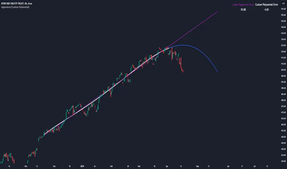
Regressing a Custom Polynomial
This library allows for fitting a custom polynomial of any form to the passed data set.
Background
The polynomial most are familiar with is where a, b and c are constants:
ax^2 + bx + c
or in a more generalizable notation where c3, c2 and c1 are constants.
c2x^2 + c1x^1 + cx^0
Polynomials are any equation of form where c1 to cn are constants:
cx^0 + c1x^1 + c2x^2 + ... + cnx^n
Note an equation like c3x^3 is still of this form because c0-c2 = 0
The library allows you fit any polynomial of this general form to a data set.

Regression with a Custom Polynomial
Steps 1, 2 and 4 from the quick start remain the same step 3 fitting the regression is where changes are made.
Pass a custom regression type and a degrees array into the fit function.

degrees = array.from(0, 3)
close_regression = regs.fit(X, y, reg.type_custom, degrees)

The degrees array corresponds to the power of each x value in the polynomial.
For example:

degrees = array.from(0, 1, 2)

This array would be the classic polynomial:
cx^0 + c1x^1 + cx^2 = ax^2 + bx + c
see each value in the array corresponds to the power of the exponent in the polynomial.

Example 2:

degrees = array.from(0, 3)

This would be a regression for a polynomial of form cx^0+ c3x*3 or ax^3 + c where a, c and c1 are constants.
Example 3:

degrees = array.from(0, 3, 7, 10)

This will regress a polynomial of form cx^0 + c3x^3 + c7x^7 + c10x^10 where c, c3, c7 and c10 are constants.

Limitations
Currently matrices cant store more than 100,000. This means the maximum length of the length of the X array multiplied by the length of the degrees array must be less than 100,000

The increasing the length of the degree array will increase computation time.

The Math Behind It
This section will quickly explain the math behind the regression. Reading this section is not needed to use the library.

This library calculates the best fitting polynomials using a least square regression. A normal equation is used to minimize the difference between the solutions vector and the x values.

A matrix is made with each column being the x array raised to the power of each exponent in the degrees array. Consider this an 'image'. The image represents all the possible solutions of multiplying the matrix by vector of real numbers. This is useful because the image is a subspace of all possible solutions to our polynomial.

This is where our y vector comes in. Our y vector will almost certainly not exist in this subspace
so we can not solve for it. So we need to find the closest vector in the solution subspace to our y vector. We do this by projecting our y vector onto the image of our solution subspace. This results in the closest vector within our solution subspace to our y vector. Now we simply need to find the coefficient vector which when multiplied by our image equals our projected vector. This coefficient vector will be the coefficients of the best fitting polynomial.

Note: Typically in linear algebra the image is denoted as A, the y vector as b and the coefficient vector as x*

Nota Keluaran:

v3

Updated:
generate_points(reg, x, y, left_index, right_index, absolute)
  Takes a regression object and creates chart points which can be used for plotting visuals like lines and labels.
  Parameters:
    reg (regression): (regression) Regression which has been fitted to a data set.
    x (array): (float) x values which coorispond to passed y values
    y (array): (float) y values which coorispond to passed x values
    left_index (int): (int) The offset of the bar farthest to the realtime bar should be larger than left_index value.
    right_index (int): (int) The offset of the bar closest to the realtime bar should be less than right_index value.
    absolute (bool)
  Returns: (chart.point) Returns an array of chart points

plot_reg(reg, x, y, left_index, right_index, absolute, curved, is_closed, line_style, line_color, line_width)
  Simple plotting function for regression for more custom plotting use generate_points() to create points then create your own plotting function.
  Parameters:
    reg (regression): (regression) Regression which has been fitted to a data set.
    x (array)
    y (array)
    left_index (int): (int) The offset of the bar farthest to the realtime bar should be larger than left_index value.
    right_index (int): (int) The offset of the bar closest to the realtime bar should be less than right_index value.
    absolute (bool)
    curved (bool): (bool) If the polyline is curved or not.
    is_closed (bool): (bool) If true the polyline will be closed.
    line_style (string)
    line_color (color): (color) The color of the line.
    line_width (int): (int) The width of the line.
  Returns: (polyline) The polyline for the regression.