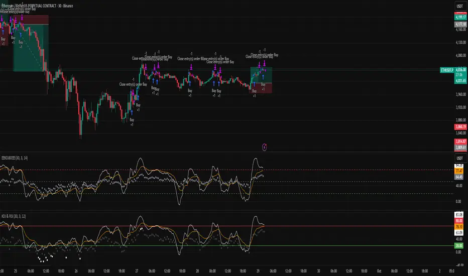
[Aegis]DCA grid Strategy for Crypto### **Crypto Market Long-Only Strategy (DCA with Risk Mitigation)**
This strategy is a Long-only approach, often using a Dollar-Cost Averaging (DCA) method for staggered entries. It is designed to mitigate the risk of being unable to exit a position for a prolonged period, which typically occurs when a series of initial DCA entries result in a losing trade.
The strategy has the following characteristics:
#### **1. Markets**
* Trade in highly liquid Perpetual Futures markets for cryptocurrencies.
#### **2. Position Sizing**
The initial entry quantity is determined by setting the **Initial Entry Ratio** in the input values.
* If the **Subsequent Entry Multiplier** is 1, the maximum position size upon final entry is determined by:
$$\text{Initial Entry Quantity} \times \text{Number of Entries}$$
* If the **Subsequent Entry Multiplier** is $x$, the maximum position size is determined by the following cumulative sum:
$$\text{1st Entry Quantity} + (\text{1st Entry Quantity} \times x) + (\text{2nd Entry Quantity} \times x) + \dots + ((\text{n-1)th Entry Quantity} \times x)$$
#### **3. Entries**
* The **1st Entry** is determined by the **Entry Sensitivity**. The first entry is automatically calculated based on an oversold condition; setting a higher sensitivity value will trigger the 1st entry in a more significant oversold situation.
* Entries from the **2nd Entry onwards** are made sequentially based on the generated **Grid Spacing**.
* The **Grid Spacing** is calculated as an equal interval:
$$\text{Grid Spacing} = \frac{\text{Final Entry Distance}}{(\text{Number of Entries} - 1)}$$
#### **4. Exits**
This strategy **does not distinguish between Stop-Loss and Take-Profit**. All entered quantities are liquidated simultaneously upon mean reversion. This transaction may result in either a loss or a profit. Generally:
* If the price recovery is rapid, the trade finishes with a profit.
* If the price recovery is slow, the trade finishes with a loss.
Therefore, the **'resilience' or 'recovery speed'** of the underlying asset significantly influences the long-term performance of the strategy.
크립토 시장에 특화된 Long only전략입니다. DCA 방식의 분할 매수 전략이 대체로 이익 거래가 아닌 경우, 장기간 탈출하지 못할 리스크를 보완한 전략입니다.
이 전략은 다음과 같은 특징을 가지고 있습니다.
##### 1. 시장 (Markets)
• 유동성이 풍부한 코인 무기한 선물 시장에서 거래한다.
##### 2. 포지션 크기 (Position Sizing)
인풋 값에 최초진입비율을 설정함으로써 1차 진입의 수량이 결정됩니다.
- 추가 진입배수가 1일 때, 최대 진입 시 포지션 크기는 "1차 진입수량 * 진입횟수"에 의해 결정됩니다.
- 추가 진입배수가 x일때,
1차진입물량 + (1차진입 물량 * x) + (2차진입 물량 * x) ..... + (n-1)차 진입물량 * x 의 방식으로 최대 진입 시 포지션 크기가 결정 됩니다
##### 3. 진입 (Entries)
- 1차 진입은 진입 둔감도에 의해 결정됩니다. 1차 진입은 과매도 상황을 자동적으로 계산하여 결정되며, 둔감도를 높은 값으로 설정하면 더 큰 과매도 상황에서 1차 진입이 결정됩니다.
- 2차 이후의 진입은 생성된 그리드 간격에 의해 순차적으로 진입하게 됩니다.
- 그리드 간격은 최종 진입 간격 / (진입 횟수 - 1) 으로 등간격으로 이루어집니다.
##### 4. 청산 (Exits)
이 전략은 손절과 익절을 구분하지 않습니다. 평균 회귀를 하는 경우 진입한 모든 물량을 일시에 청산하며, 이 거래는 손실 거래일 수도, 이익 거래일 수도 있습니다. 일반적으로, 가격 회복이 빠르게 되는 경우 이익 거래로 마무리되고, 가격 회복이 느린 경우 손실 거래로 마무리되기 때문에, 장기적으로 종목의 '회복탄력성'이 전략의 성과에 영향을 줄 수 있습니다.
Ketidakstabilan

[Aegis]Original Turtle System for CryptoAs Richard Dennis once said, "Even if I published all the Turtle rules in the newspaper right now, no one would be able to 'execute' them," and 40 years later, even in modern financial markets (like the crypto market) where all the conditions have been disclosed, this strategy continues to deliver amazing performance. The following outlines the original Turtle rules as disclosed by Curtis Faith in his book *Way of the Turtle*, and a TradingView algorithm that translates these rules for application in the crypto market.
---
### **The Original Turtle Trading Rules**
#### **1. Markets**
* Trade in liquid futures markets.
#### **2. Position Sizing**
The volatility measure, **N**, is used as the basis for all calculations.
**True Range (TR) Calculation:** Select the largest of the following three values:
* Current High - Current Low
* $|\text{Current High} - \text{Previous Close}|$ (Absolute Value)
* $|\text{Current Low} - \text{Previous Close}|$ (Absolute Value)
**N (Average True Range, ATR) Calculation:**
$$N = \frac{(19 \times \text{PDN} + \text{TR})}{20}$$
* **PDN:** Previous Day's N value
* **TR:** Current True Range
This is similar to a 20-day Exponential Moving Average, and is sometimes calculated using a Simple Moving Average.
**Unit Size Calculation:**
$$\text{Unit Size (Number of Contracts)} = \frac{1\% \text{ of Account Equity}}{(\text{N} \times \text{Dollars per Point})}$$
* **Dollars per Point (Tick Value):** The value of a 1-point change in price.
#### **3. Entries**
* **Entry:** Buy when the 55-day high is broken to the upside, and sell when the 55-day low is broken to the downside.
#### **5. Stops**
* The stop-loss for every unit is set at a price **2N** unfavorable from the entry price.
* For each additional unit added, the stop price for the **entire position** is adjusted favorably by **1/2 N**.
* In other words, the stop price of the last unit entered becomes the stop price for the entire position.
#### **6. Exits**
The exit rule for profitable positions (before a stop is hit) is as follows:
* **Long Positions:** Exit when the 20-day low is broken to the downside.
* **Short Positions:** Exit when the 20-day high is broken to the upside.
*Note: This exit rule is followed only if the price has moved up by a value greater than or equal to the N value multiplied by the criterion for changing the take-profit line (the original Korean text mentions a condition based on N, which is commonly interpreted as requiring a profit before applying the channel exit).*
리처드 데니스가 앞서 "내가 지금 당장 터틀의 모든 규칙을 신문에 공표한다고 해도 아무도 '실행'하지 못할 것"라고 말했듯 40년이 흘러 모든 조건이 공개된 현대 금융시장(크립토 시장)에서도 여전히 이 전략은 놀라운 퍼포먼스를 기록하고 있습니다. 아래는 커티스 페이스가 자신의 저서 '터틀의 방식'에 공개한 오리지널 터틀 규칙과 이를 알고리즘으로 변환하여 크립토마켓에 적용한 트레이딩뷰 알고리즘 입니다.
##### 1. 시장 (Markets)
• 유동성이 풍부한 선물 시장에서 거래한다.
##### 2. 포지션 크기 (Position Sizing)
변동성 측정 단위인 N을 모든 계산의 기초로 사용한다.
**True Range (TR) 계산:** 다음 세 가지 값 중 가장 큰 값을 선택한다.
- • 현재 고가 - 현재 저가
- • |현재 고가 - 전일 종가| (절대값)
- • |현재 저가 - 전일 종가| (절대값)
**N (Average True Range, ATR) 계산:**
N = (19 × PDN + TR) / 20
- • PDN: 이전 날의 N 값
- • TR: 현재 True Range
이는 20일 지수이동평균과 유사하며, 단순이동평균으로 계산하기도 한다.
**1 유닛(Unit)의 크기 계산:**
유닛 크기 (계약 수) = 계좌 자산의 1% / (N × 틱 가치)
• 틱 가치(Dollars per Point): 1포인트 변동 시의 가치
##### 3. 진입 (Entries)
- • 진입: 55일 고가를 상향 돌파하면 매수, 55일 저가를 하향 돌파하면 매도한다.
##### 5. 손절 (Stops)
- • 모든 유닛에 대한 손절 기준은 진입 가격으로부터 2N 만큼 불리한 가격에 설정한다.
- • 유닛이 추가될 때마다 전체 포지션의 손절 가격을 1/2 N 만큼 유리한 방향으로 상향 조정한다.
- • 즉, 마지막으로 진입한 유닛의 손절 가격이 전체 포지션의 손절 가격이 된다.
##### 6. 청산 (Exits)
손절에 도달하기 전 수익 중인 포지션의 청산 규칙은 다음과 같다.
- • 매수 포지션: 20일 저가를 하향 돌파할 때 청산한다.
- • 매도 포지션: 20일 고가를 상향 돌파할 때 청산한다.
단, N값에 익절선 변경 기준을 곱한 값 이상으로 가격이 상승할 경우, 위 규칙을 따른다.

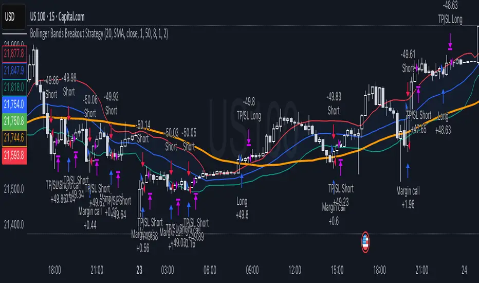
Bollinger Bands Breakout StrategyHey guys check out this strategy script.
Chart plotting:
I use a classic plot of Bollinger Bands to define a consolidation zone, I also use a separate Trend Filter (SMA).
Logic:
When the price is above the SMA and above the Bollinger Upper Band the strategy goes Long. When the price is below the SMA and below the Bollinger Lower Band the strategy goes Short. Simple.
Exits:
TP and SL are a percentage of the price.
Notes: This simple strategy can be used at any timeframe (I prefer the 15min for day trading). It avoids consolidation, when the price is inside the Bollinger Bands, and has a good success rate. Adjust the Length of the BB to suit your style of trading (Lower numbers=more volatile, Higher numbers=more restrictive). Also you can adjust the Trend Filter SMA, I presonally chose the 50 SMA. Finally the SL/TP can be also adjusted from the input menu.
Test it for yourself!
Have great trades!
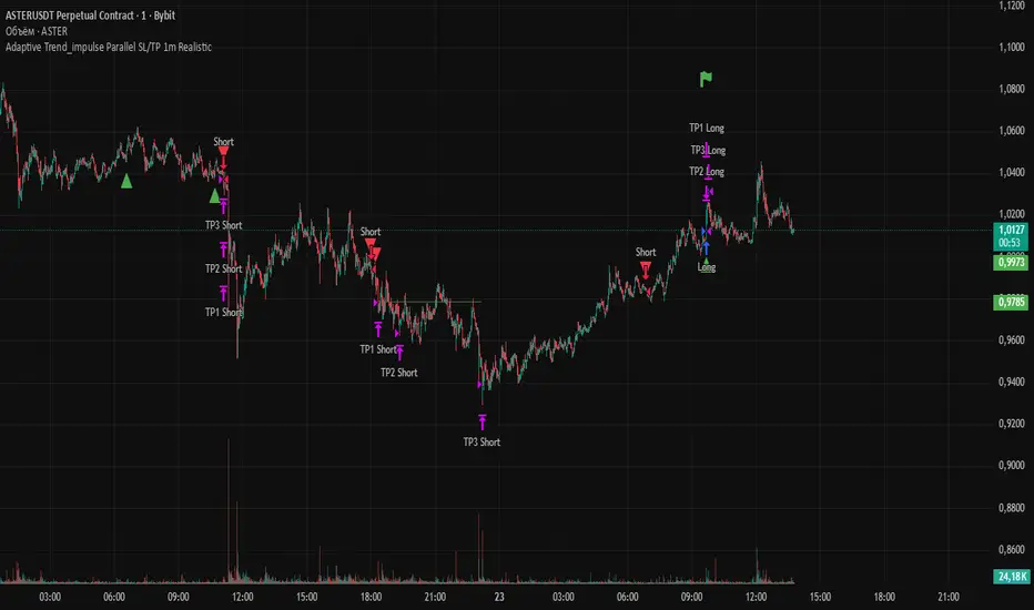
Adaptive Trend 1m ### Overview
The "Adaptive Trend Impulse Parallel SL/TP 1m Realistic" strategy is a sophisticated trading system designed specifically for high-volatility markets like cryptocurrencies on 1-minute timeframes. It combines trend-following with momentum filters and adaptive parameters to dynamically adjust to market conditions, ensuring more reliable entries and risk management. This strategy uses SuperTrend for primary trend detection, enhanced by MACD, RSI, Bollinger Bands, and optional volume spikes. It incorporates parallel stop-loss (SL) and multiple take-profit (TP) levels based on ATR, with options for breakeven and trailing stops after the first TP. Optimized for realistic backtesting on short timeframes, it avoids over-optimization by adapting indicators to market speed and efficiency.
### Principles of Operation
The strategy operates on the principle of adaptive impulse trading, where entry signals are generated only when multiple conditions align to confirm a strong trend reversal or continuation:
1. **Trend Detection (SuperTrend)**: The core signal comes from an adaptive SuperTrend indicator. It calculates upper and lower bands using ATR (Average True Range) with dynamic periods and multipliers. A buy signal occurs when the price crosses above the lower band (from a downtrend), and a sell signal when it crosses below the upper band (from an uptrend). Adaptation is based on Rate of Change (ROC) to measure market speed, shortening periods in fast markets for quicker responses.
2. **Momentum and Trend Filters**:
- **MACD**: Uses adaptive fast and slow lengths. In "Trend Filter" mode (default when "Use MACD Cross" is false), it checks if the MACD line is above/below the signal for long/short. In cross mode, it requires a crossover/crossunder.
- **RSI**: Adaptive period RSI must be above 50 for longs and below 50 for shorts, confirming overbought/oversold conditions dynamically.
- **Bollinger Bands (BB)**: Depending on the mode ("Midline" by default), it requires the price to be above/below the BB midline for longs/shorts, or a breakout in "Breakout" mode. Deviation adapts to market efficiency.
- **Volume Spike Filter** (optional): Entries require volume to exceed an adaptive multiple of its SMA, signaling strong impulse.
3. **Volatility Filter**: Entries are only allowed if current ATR percentage exceeds a historical minimum (adaptive), preventing trades in low-volatility ranges.
4. **Risk Management (Parallel SL/TP)**:
- **Stop-Loss**: Set at an adaptive ATR multiple below/above entry for long/short.
- **Take-Profits**: Three levels at adaptive ATR multiples, with partial position closures (e.g., 51% at TP1, 25% at TP2, remainder at TP3).
- **Post-TP1 Features**: Optional breakeven moves SL to entry after TP1. Trailing SL uses BB midline as a dynamic trail.
- All levels are calculated per trade using the ATR at entry, making them "realistic" for 1m charts by widening SL and tightening initial TPs.
The strategy enters long on buy signals with all filters met, and short on sell signals. It uses pyramid margin (100% long/short) for full position sizing.
Adaptation is driven by:
- **Market Speed (normSpeed)**: Based on ROC, tightens multipliers in volatile periods.
- **Efficiency Ratio (ER)**: Measures trend strength, adjusting periods for trending vs. ranging markets.
This ensures the strategy "adapts" without manual tweaks, reducing false signals in varying conditions.
### Main Advantages
- **Adaptability**: Unlike static strategies, parameters dynamically adjust to market volatility and trend strength, improving performance across ranging and trending phases without over-optimization.
- **Realistic Risk Management for 1m**: Wider SL and tiered TPs prevent premature stops in noisy short-term charts, while partial profits lock in gains early. Breakeven/trailing options protect profits in extended moves.
- **Multi-Filter Confirmation**: Combines trend, momentum, and volume for high-probability entries, reducing whipsaws. The volatility filter avoids flat markets.
- **Debug Visualization**: Built-in plots for signals, levels, and component checks (when "Show Debug" is enabled) help users verify logic on charts.
- **Efficiency**: Low computational load, suitable for real-time trading on TradingView with alerts.
Backtesting shows robust results on volatile assets, with a focus on sustainable risk (e.g., SL at 3x ATR avoids excessive drawdowns).
### Uniqueness
What sets this strategy apart is its **fully adaptive framework** integrating multiple indicators with real-time market metrics (ROC for speed, ER for efficiency). Most trend strategies use fixed parameters, leading to poor adaptation; here, every key input (periods, multipliers, deviations) scales dynamically within bounds, creating a "self-tuning" system. The "parallel SL/TP with 1m realism" adds custom handling for micro-timeframes: tightened initial TPs for quick wins and adaptive min-ATR filter to skip low-vol bars. Unlike generic mashups, it justifies the combination—SuperTrend for trend, MACD/RSI/BB for impulse confirmation, volume for conviction—working synergistically to capture "trend impulses" while filtering noise. The post-TP1 breakeven/trailing tied to BB adds a unique profit-locking mechanism not common in open-source scripts.
### Recommended Settings
These settings are optimized and recommended for trading ASTER/USDT on Bybit, with 1-minute chart, x10 leverage, and cross margin mode. They provide a balanced risk-reward for this volatile pair:
- **Base Inputs**:
- Base ATR Period: 10
- Base SuperTrend ATR Multiplier: 2.5
- Base MACD Fast: 8
- Base MACD Slow: 17
- Base MACD Signal: 6
- Base RSI Period: 9
- Base Bollinger Period: 12
- Bollinger Deviation: 1.8
- Base Volume SMA Period: 19
- Base Volume Spike Multiplier: 1.8
- Adaptation Window: 54
- ROC Length: 10
- **TP/SL Settings**:
- Use Stop Loss: True
- Base SL Multiplier (ATR): 3
- Use Take Profits: True
- Base TP1 Multiplier (ATR): 5.5
- Base TP2 Multiplier (ATR): 10.5
- Base TP3 Multiplier (ATR): 19
- TP1 % Position: 51
- TP2 % Position: 25
- Breakeven after TP1: False
- Trailing SL after TP1: False
- Base Min ATR Filter: 0.001
- Use Volume Spike Filter: True
- BB Condition: Midline
- Use MACD Cross (false=Trend Filter): True
- Show Debug: True
For backtesting, use initial capital of 30 USD, base currency USDT, order size 100 USDT, pyramiding 1, commission 0.1%, slippage 0 ticks, long/short margin 0%.
Always backtest on your platform and use risk management—risk no more than 1-2% per trade. This is not financial advice; trade at your own risk.
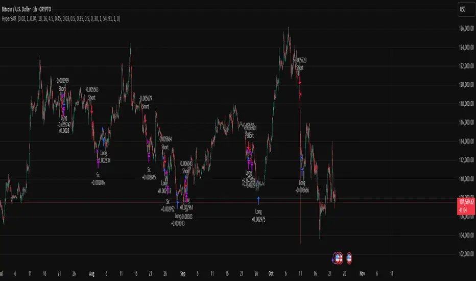
Hyper SAR Reactor Trend StrategyHyperSAR Reactor Adaptive PSAR Strategy
Summary
Adaptive Parabolic SAR strategy for liquid stocks, ETFs, futures, and crypto across intraday to daily timeframes. It acts only when an adaptive trail flips and confirmation gates agree. Originality comes from a logistic boost of the SAR acceleration using drift versus ATR, plus ATR hysteresis, inertia on the trail, and a bear-only gate for shorts. Add to a clean chart and run on bar close for conservative alerts.
Scope and intent
• Markets: large cap equities and ETFs, index futures, major FX, liquid crypto
• Timeframes: one minute to daily
• Default demo: BTC on 60 minute
• Purpose: faster yet calmer PSAR that resists chop and improves short discipline
• Limits: this is a strategy that places simulated orders on standard candles
Originality and usefulness
• Novel fusion: PSAR AF is boosted by a logistic function of normalized drift, trail is monotone with inertia, entries use ATR buffers and optional cooldown, shorts are allowed only in a bear bias
• Addresses false flips in low volatility and weak downtrends
• All controls are exposed in Inputs for testability
• Yardstick: ATR normalizes drift so settings port across symbols
• Open source. No links. No solicitation
Method overview
Components
• Adaptive AF: base step plus boost factor times logistic strength
• Trail inertia: one sided blend that keeps the SAR monotone
• Flip hysteresis: price must clear SAR by a buffer times ATR
• Volatility gate: ATR over its mean must exceed a ratio
• Bear bias for shorts: price below EMA of length 91 with negative slope window 54
• Cooldown bars optional after any entry
• Visual SAR smoothing is cosmetic and does not drive orders
Fusion rule
Entry requires the internal flip plus all enabled gates. No weighted scores.
Signal rule
• Long when trend flips up and close is above SAR plus buffer times ATR and gates pass
• Short when trend flips down and close is below SAR minus buffer times ATR and gates pass
• Exit uses SAR as stop and optional ATR take profit per side
Inputs with guidance
Reactor Engine
• Start AF 0.02. Lower slows new trends. Higher reacts quicker
• Max AF 1. Typical 0.2 to 1. Caps acceleration
• Base step 0.04. Typical 0.01 to 0.08. Raises speed in trends
• Strength window 18. Typical 10 to 40. Drift estimation window
• ATR length 16. Typical 10 to 30. Volatility unit
• Strength gain 4.5. Typical 2 to 6. Steepness of logistic
• Strength center 0.45. Typical 0.3 to 0.8. Midpoint of logistic
• Boost factor 0.03. Typical 0.01 to 0.08. Adds to step when strength rises
• AF smoothing 0.50. Typical 0.2 to 0.7. Adds inertia to AF growth
• Trail smoothing 0.35. Typical 0.15 to 0.45. Adds inertia to the trail
• Allow Long, Allow Short toggles
Trade Filters
• Flip confirm buffer ATR 0.50. Typical 0.2 to 0.8. Raise to cut flips
• Cooldown bars after entry 0. Typical 0 to 8. Blocks re entry for N bars
• Vol gate length 30 and Vol gate ratio 1. Raise ratio to trade only in active regimes
• Gate shorts by bear regime ON. Bear bias window 54 and Bias MA length 91 tune strictness
Risk
• TP long ATR 1.0. Set to zero to disable
• TP short ATR 0.0. Set to 0.8 to 1.2 for quicker shorts
Usage recipes
Intraday trend focus
Confirm buffer 0.35 to 0.5. Cooldown 2 to 4. Vol gate ratio 1.1. Shorts gated by bear regime.
Intraday mean reversion focus
Confirm buffer 0.6 to 0.8. Cooldown 4 to 6. Lower boost factor. Leave shorts gated.
Swing continuation
Strength window 24 to 34. ATR length 20 to 30. Confirm buffer 0.4 to 0.6. Use daily or four hour charts.
Properties visible in this publication
Initial capital 10000. Base currency USD. Order size Percent of equity 3. Pyramiding 0. Commission 0.05 percent. Slippage 5 ticks. Process orders on close OFF. Bar magnifier OFF. Recalculate after order filled OFF. Calc on every tick OFF. No security calls.
Realism and responsible publication
No performance claims. Past results never guarantee future outcomes. Shapes can move while a bar forms and settle on close. Strategies execute only on standard candles.
Honest limitations and failure modes
High impact events and thin books can void assumptions. Gap heavy symbols may prefer longer ATR. Very quiet regimes can reduce contrast and invite false flips.
Open source reuse and credits
Public domain building blocks used: PSAR concept and ATR. Implementation and fusion are original. No borrowed code from other authors.
Strategy notice
Orders are simulated on standard candles. No lookahead.
Entries and exits
Long: flip up plus ATR buffer and all gates true
Short: flip down plus ATR buffer and gates true with bear bias when enabled
Exit: SAR stop per side, optional ATR take profit, optional cooldown after entry
Tie handling: stop first if both stop and target could fill in one bar
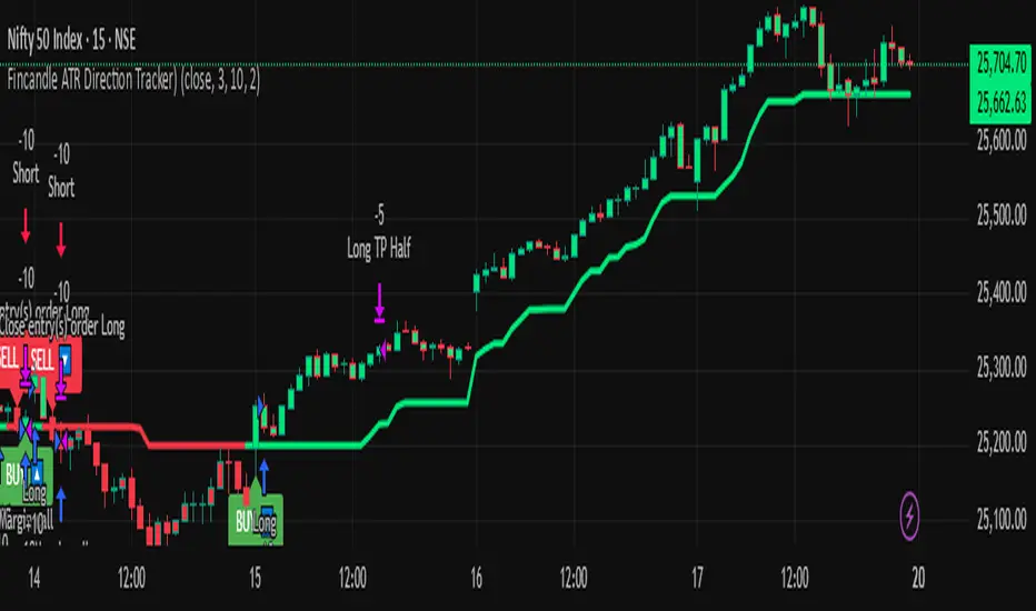
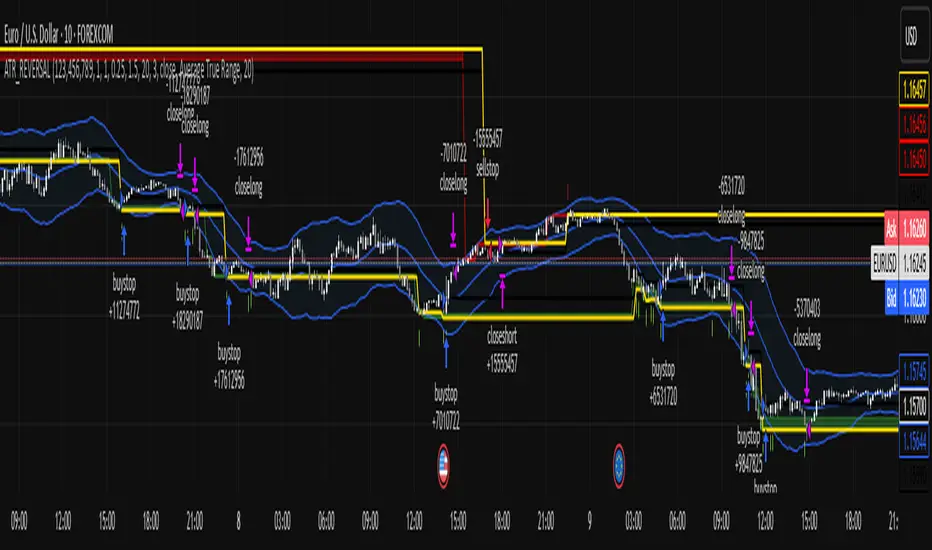
Fincandle ATR Direction TrackerOverview
The Fincandle ATR Direction Tracker is a strategy designed to capture momentum moves in the market using a dynamic ATR-based trailing stop. It identifies strong momentum candles and filters signals using trend alignment with moving averages.
Partial exits allow users to take a portion of profit at a predefined ATR multiple while keeping the remaining position open until the opposite signal occurs.
How It Works
Momentum Detection:
Measures candle body size relative to the Average True Range (ATR).
A candle is considered momentum if its body size exceeds ATR × Multiplier.
Trend Filter:
Uses two moving averages (Fast MA and Slow MA) to determine the market trend.
Bullish trend: Fast MA > Slow MA → long trades allowed
Bearish trend: Fast MA < Slow MA → short trades allowed
Trend filter can be toggled on or off.
ATR Trailing Stop:
A dynamic trailing stop adapts to price volatility.
Crossing above the trail triggers a buy signal, crossing below triggers a sell signal.
Partial Exit / Take Profit:
Step 1: Exit 50% of the position when price moves a configurable multiple of ATR in your favor.
Step 2: Close the remaining position when the opposite signal occurs (e.g., price crosses below/above the ATR trail).
How to Use
Add the strategy to any chart (stocks, indices, forex, crypto).
Configure ATR period, sensitivity, take profit multiple, and moving average lengths to suit the timeframe and asset.
Monitor buy/sell markers and dynamic ATR trail on the chart.
Optional: Set alerts for real-time notifications when signals trigger.
Adjust partial exit multiplier to control risk/reward.
Example Settings
ATR Period: 10
ATR Sensitivity: 3 × ATR
Take Profit: 2 × ATR
Fast MA: 50
Slow MA: 200
Partial Exit: 50% of position at take profit, remaining exits on opposite signal
Key Features
Adaptive ATR trailing stop for volatility-based entries/exits.
Trend alignment filter with Fast/Slow MA.
Partial exit logic for better risk management.
Visual BUY/SELL markers and alerts.
Fully Pine Script v6 compatible.
Disclaimer
This strategy is for educational and analytical purposes only.
It does not guarantee profits. Traders should always use proper risk management.
5min ORB with FVG God Modethis is 15 min Order Block strategy who works verry well on 3 min chart just must to close some
trading hours

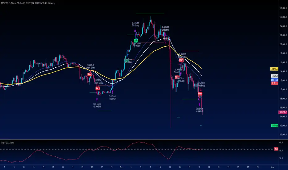
Turtle Strategy - Triple EMA Trend with ADX and ATRDescription
The Triple EMA Trend strategy is a directional momentum system built on the alignment of three exponential moving averages and a strong ADX confirmation filter. It is designed to capture established trends while maintaining disciplined risk management through ATR-based stops and targets.
Core Logic
The system activates only under high-trend conditions, defined by the Average Directional Index (ADX) exceeding a configurable threshold (default: 43).
A bullish setup occurs when the short-term EMA is above the mid-term EMA, which in turn is above the long-term EMA, and price trades above the fastest EMA.
A bearish setup is the mirror condition.
Execution Rules
Entry:
• Long when ADX confirms trend strength and EMA alignment is bullish.
• Short when ADX confirms trend strength and EMA alignment is bearish.
Exit:
• Stop Loss: 1.8 × ATR below (for longs) or above (for shorts) the entry price.
• Take Profit: 3.3 × ATR in the direction of the trade.
Both parameters are configurable.
Additional Features
• Start/end date inputs for controlled backtesting.
• Selective activation of long or short trades.
• Built-in commission and position sizing (percent of equity).
• Full visual representation of EMAs, ADX, stop-loss, and target levels.
This strategy emphasizes clean trend participation, strict entry qualification, and consistent reward-to-risk structure. Ideal for swing or medium-term testing across trending assets.
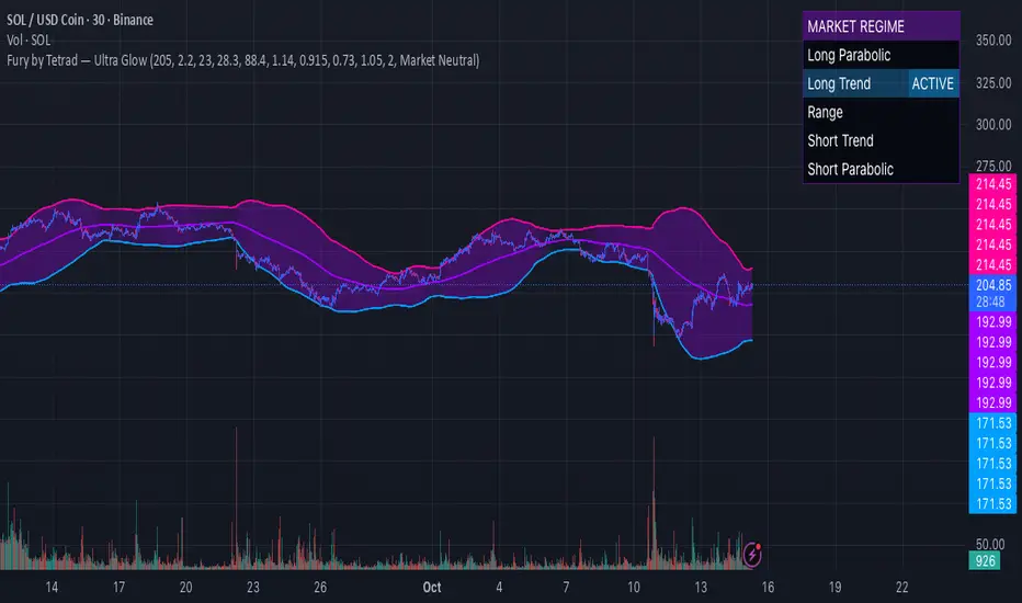
Fury by Tetrad Fury by Tetrad
What it is:
A rules-based Bollinger+RSI strategy that fades extremes: it looks for price stretching beyond Bollinger Bands while RSI confirms exhaustion, enters countertrend, then exits at predefined profit multipliers or optional stoploss. “Ultra Glow” visuals are purely cosmetic.
How it works — logic at a glance
Framework: Classic Bollinger Bands (SMA basis; configurable length & multiplier) + RSI (configurable length).
Long entries:
Price closes below the lower band and RSI < Long RSI threshold (default 28.3) → open LONG (subject to your “Market Direction” setting).
Short entries:
Price closes above the upper band and RSI > Short RSI threshold (default 88.4) → open SHORT.
Profit exits (price targets):
Uses simple multipliers of the strategy’s average entry price:
Long exit = `entry × Long Exit Multiplier` (default 1.14).
Short exit = `entry × Short Exit Multiplier` (default 0.915).
Risk controls:
Optional pricebased stoploss (disabled by default) via:
Long stop = `entry × Long Stop Factor` (default 0.73).
Short stop = `entry × Short Stop Factor` (default 1.05).
Directional filter:
“Market Direction” input lets you constrain entries to Market Neutral, Long Only, or Short Only.
Visuals:
“Ultra Glow” draws thin layered bands around upper/basis/lower; these do not affect signals.
> Note: Inputs exist for a timebased stop tracker in code, but this version exits via targets and (optional) price stop only.
Why it’s different / original
Explicit extreme + momentum pairing: Entries require simultaneous band breach and RSI exhaustion, aiming to avoid entries on gardenvariety volatility pokes.
Deterministic exits: Multiplier-based targets keep results auditable and reproducible across datasets and assets.
Minimal, unobtrusive visuals: Thin, layered glow preserves chart readability while communicating regime around the Bollinger structure.
Inputs you can tune
Bollinger: Length (default 205), Multiplier (default 2.2).
RSI: Length (default 23), Long/Short thresholds (28.3 / 88.4).
Targets: Long Exit Mult (1.14), Short Exit Mult (0.915).
Stops (optional): Enable/disable; Long/Short Stop Factors (0.73 / 1.05).
Market Direction: Market Neutral / Long Only / Short Only.
Visuals: Ultra Glow on/off, light bar tint, trade labels on/off.
How to use it
1. Timeframe & assets: Works on any symbol/timeframe; start with liquid majors and 60m–1D to establish baseline behavior, then adapt.
2. Calibrate thresholds:
Narrow/meanreverting markets often tolerate tighter RSI thresholds.
Fast/volatile markets may need wider RSI thresholds and stronger stop factors.
3. Pick realistic targets: The default multipliers are illustrative; tune them to reflect typical mean reversion distance for your instrument/timeframe (e.g., ATRinformed profiling).
4. Risk: If enabling stops, size positions so risk per trade ≤ 1–2% of equity (max 5–10% is a commonly cited upper bound).
5. Mode: Use Long Only or Short Only when your discretionary bias or higher timeframe model favors one side; otherwise Market Neutral.
Recommended publication properties (for backtests that don’t mislead)
When you publish, set your strategy’s Properties to realistic values and keep them consistent with this description:
Initial capital: 10,000 (typical retail baseline).
Commission: ≥ 0.05% (adjust for your venue).
Slippage: ≥ 2–3 ticks (or a conservative pertrade value).
Position sizing: Avoid risking > 5–10% equity per trade; fixedfractional sizing ≤ 10% or fixedcash sizing is recommended.
Dataset / sample size: Prefer symbols/timeframes yielding 100+ trades over the tested period for statistical relevance. If you deviate, say why.
> If you choose different defaults (e.g., capital, commission, slippage, sizing), explain and justify them here, and use the same settings in your publication.
Interpreting results & limitations
This is a countertrend approach; it can struggle in strong trends where band breaches compound.
Parameter sensitivity is real: thresholds and multipliers materially change trade frequency and expectancy.
No predictive claims: Past performance is not indicative of future results. The future is unknowable; treat outputs as decision support, not guarantees.
Suggested validation workflow
Try different assets. (TSLA, AAPL, BTC, SOL, XRP)
Run a walkforward across multiple years and market regimes.
Test several timeframes and multiple instruments. (30m Suggested)
Compare different commission/slippage assumptions.
Inspect distribution of returns, max drawdown, win/loss expectancy, and exposure.
Confirm behavior during trend vs. range segments.
Alerts & automation
This release focuses on chart execution and visualization. If you plan to automate, create alerts at your entry/exit conditions and ensure your broker/venue fills reflect your slippage/fees assumptions.
Disclaimer
This script is provided for educational and research purposes. It is not investment advice. Trading involves risk, including the possible loss of principal. © Tetrad Protocol.
SabinaCounter-trend strategy working only in long.
Principle of Operation
The strategy is based on market extremes, which serve as both the signals for opening a position and for closing it. These extremes possess data such as Open, High, Low, Close, and others. The length and the shift (positive or negative) of the extremes are also configurable.
The extreme Ext is used for closing the position, and the extreme Ent is used for opening the position.
Base Order
A dedicated percentage of the deposit is specified. If the price crosses the Ent extreme, a long position is opened.
Take Profit and Stop Loss
The Take Profit level is calculated from the average price. A trailing stop order is present by default, which is set by the Ext extreme. When the price crosses this extreme, the position will be closed if the Take Profit has not yet been reached.
Grid of Orders (Averaging)
This section allows for enabling or disabling the grid of orders.
In the order grid, you can specify the percentage below the base order at which the grid's limit orders should be placed. The grid step is also configurable. The leverage for all orders, including the base order, is set here.
The order grid consists of 10 orders, and each order can be assigned its own percentage of the deposit. This gives the strategy greater flexibility compared to a standard DCA (Dollar-Cost Averaging) grid.
Information Panel
A table displays the historical price drop at a given moment, providing some insight into the potential liquidation level based on the selected leverage. The table also shows the deposit utilization (how much of the deposit is currently tied up).

Squeeze Backtest by Shaqi v2.0Script to backtest price squeeze's. Works on long and short directions

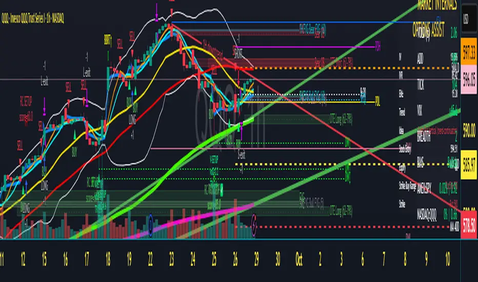
Trend-Following & Breakout — Index Quant Strategy (NASDAQ)📈 Trend-Following & Breakout — Index Quant Strategy (NASDAQ & S&P 500)
Type: Invite-only strategy
Markets: NASDAQ 100 (NAS100 / US100 / NQ), S&P 500 (US500 / SPX), and other major equity indices.
🧠 Concept: Continuous trend model combining EWMAC (trend-following) and Donchian (breakout) signals, scaled by forecast strength and portfolio risk.
⚙️ Execution: Rebalances only on decision-bar closes, using hysteresis and a no-trade band to reduce churn.
📊 Default bias: Long-only — aligned with equity index drift.
🧩 How it works
• EWMAC Trend: Difference between fast and slow EMAs, normalized by an EWMA of absolute returns.
• Donchian Breakout: Distance beyond a 200-bar channel (Strict mode) or relative z-score position within it.
• Forecast combination: Weighted sum of trend and breakout points, clamped to ± capPoints.
• Hysteresis: Prevents quick sign flips near zero forecast.
• Risk scaling: Maps forecast strength to position size using equity × risk budget × ATR-based stop distance.
• Rebalance: Executes only if the required quantity change exceeds the Δqty threshold; can optionally block increases on Sundays (for CFDs).
⚙️ Default parameters
Deployed on NQ / US100 / NAS100 on Daily Timeframe
• Decision timeframe = 360 min (other options from 1 min to 1 week).
• Trend (EWMAC): Fast = 64, Slow = 256, Vol Norm = 32, Weight = 0.8.
• Breakout (Donchian): Length = 200, Mode = Strict, Weight = 0.2.
• Forecast scaling: ptsPerSigma = 1.0, capPoints = 10.
• Risk % per rebalance = 4 % of equity.
• ATR stop: ATR(14) × 1.0.
• No-trade band (Δqty) = 4 units.
• Hysteresis = 2 forecast points.
• Bias = Long-only (Neutral / Long-bias 50 % optional).
• Skip Sunday increases = false (default).
📋 Backtest properties (documented)
• Initial capital = 100 000 USD.
• Commission = 0.20 % per trade.
• Pyramiding = 10.
• Calc on every tick = false.
• Point value = 1 (for NAS100 CFD).
• No financing or slippage modeled.
• If using CFDs, account for overnight funding.
• On futures (NQ / ES), carry is implicit.
📊 Typical behaviour
• Many small scratches, a few large winners.
• Performs best during multi-week / multi-month trends.
• Underperforms in tight or volatile ranges.
• Average hold ≈ 30 – 90 days in historical tests.
💡 Risk and performance guide (illustrative)
Sharpe ≈ 1.25
Sortino ≈ 1.10 – 1.30
Max drawdown ≈ –18 % to –25 %
Annual volatility ≈ 24 – 28 %
CAGR ≈ 50 – 60 % (at 4 % risk)
Edge ratio ≈ 5 (MFE / MAE)
Historical backtests only — past performance does not guarantee future results.
🌍 Intended markets and timeframes
Optimized for NASDAQ 100 and S&P 500; also effective on similar indices (DAX, Dow Jones, FTSE).
Best on Daily or higher timeframes.
Aligns with long-term index drift — suitable for long-bias systematic trend portfolios.
⚠️ Limitations
• Backtests exclude CFD funding costs.
• Trend models will have losing streaks in range-bound markets.
• Designed for experienced traders seeking systematic exposure.
🔑 Requesting access
Send a private TradingView message to with the text:
“Request access to Trend-Following & Breakout — Index Quant Strategy.”
Access is granted only on explicit request.
For further information, see my TradingView Signature.
🆕 Release notes (v1.0)
• Initial release (360 min TF): EWMAC 64/256 + Donchian 200 Strict.
• Risk 4 %, ATR × 1.0, Long-only bias, hysteresis 2 pts, Δqty ≥ 4.
• Developed for NASDAQ 100 and S&P 500 indices.
• Implements continuous risk-scaled positioning and no-trade band logic.
🧾 Originality statement
This strategy is original work built entirely from TradingView built-ins (EMA, ATR, Highest, Lowest).
It does not reuse open-source invite-only code.
Any future reuse of open scripts will be done with explicit permission and credit.

Universal Breakout Strategy [KedArc Quant]Description:
A flexible breakout framework where you can test different logics (Prev Day, Bollinger, Volume, ATR, EMA Trend, RSI Confirm, Candle Confirm, Time Filter) under one system.
Choose your breakout mode, and the strategy will handle entries, exits, and optional risk management (ATR stops, take-profits, daily loss guard, cooldowns).
An on-chart info table shows live mode values (like Prev High/Low, Bollinger levels, RSI, etc.) plus P&L stats for quick analysis.
Use it to compare which breakout style works best on your instrument and timeframe, whether intraday, swing, or positional trading
🔑 Why it’s useful
* Flexibility: Switch between breakout strategies without loading different indicators.
* Clarity: On-chart info table displays current mode, relevant indicator levels, and live strategy P&L stats.
* Testing efficiency: Quickly A/B test different breakout styles under the same backtest environment.
* Transparency: Every trade is rule-based and displayed with entry/exit markers.
🚀 How it helps traders
* Lets you experiment with breakout strategies quickly without loading multiple scripts.
* Helps identify which breakout method fits your instrument & timeframe.
* Gives clear on-chart visual + statistical feedback for confident decision-making.
⚙️ Input Configuration
* Breakout Mode → choose which strategy to test:
* *Prev Day* → breakouts of yesterday’s High/Low.
* *Bollinger* → Upper/Lower BB pierce.
* *Volume* → Breakout confirmed with volume above average.
* *ATR Stop* → Wide range breakout using ATR filter.
* *Time Filter* → Breakouts inside defined session hours.
* *EMA Trend* → Breakouts only in EMA fast > slow alignment.
* *RSI Confirm* → Breakouts with RSI confirmation (e.g. >55 for longs).
* *Candle Confirm* → Breakouts validated by bullish/bearish candle.
* Lookback / ATR / Bollinger inputs → adjust sensitivity.
* Intrabar mode → option to evaluate breakouts using bar highs/lows instead of closes.
* Table options → show/hide info table, show/hide P&L stats, choose corner placement.
📈 Entry & Exit Logic
* Entry → occurs when breakout condition of chosen mode is met.
* Exit → default exits via opposite signals or optional stop/target if enabled.
* Session filter → optional auto-flat at session end.
* P&L management → optional daily loss guard, cooldown between trades, and ATR-based stop/take profit.
❓ FAQ — Choosing the best setup
Q: Which strategy should I use for which chart?
* *Prev Day Breakouts*: Best on indices, FX, and liquid futures with strong daily levels.
* *Bollinger*: Works well in range-bound environments, or crypto pairs with volatility compression.
* *Volume*: Good on equities where breakout strength is tied to volume spikes.
* *ATR Stop*: Suits volatile instruments (commodities, crypto).
* *EMA Trend*: Useful in trending markets (stocks, indices).
* *RSI Confirm*: Adds momentum filter, better for swing trades.
* *Candle Confirm*: Ideal for scalpers needing visual confirmation.
* *Time Filter*: For intraday traders who want signals only in high-liquidity sessions.
Q: What timeframe should I use?
* Intraday traders → 5m to 15m (Time Filter, Candle Confirm).
* Swing traders → 1H to 4H (EMA Trend, RSI Confirm, ATR Stop).
* Position traders → Daily (Prev Day, Bollinger).
* Breakout
A trade entry condition triggered when price crosses above a resistance level (for longs) or below a support level (for shorts).
* Prev Day High/Low
Formula:
Prev High = High of (Day )
Prev Low = Low of (Day )
* Bollinger Bands
Formula:
Basis = SMA(Close, Length)
Upper Band = Basis + (Multiplier × StdDev(Close, Length))
Lower Band = Basis – (Multiplier × StdDev(Close, Length))
* Volume Confirmation
A breakout is only valid if:
Volume > SMA(Volume, Length)
* ATR (Average True Range)
Measures volatility.
Formula:
ATR = SMA(True Range, Length)
where True Range = max(High–Low, |High–Close |, |Low–Close |)
* EMA (Exponential Moving Average)
Weighted moving average giving more weight to recent prices.
Formula:
EMA = (Price × α) + (EMA × (1–α))
with α = 2 / (Length + 1)
* RSI (Relative Strength Index)
Momentum oscillator scaled 0–100.
Formula:
RSI = 100 – (100 / (1 + RS))
where RS = Avg(Gain, Length) ÷ Avg(Loss, Length)
* Candle Confirmation
Bullish candle: Close > Open AND Close > Close
Bearish candle: Close < Open AND Close < Close
Win Rate (%)
Formula:
Win Rate = (Winning Trades ÷ Total Trades) × 100
* Average Trade P&L
Formula:
Avg Trade = Net Profit ÷ Total Trades
📊 Performance Notes
The Universal Breakout Strategy is designed as a framework rather than a single-asset optimized system. Results will vary depending on the chart, timeframe, and asset chosen.
On the current defaults (15-minute, INR-denominated example), the backtest produced 132 trades over the selected period. This provides a statistically sufficient sample size.
Win rate (~35%) is relatively low, but this is balanced by a positive reward-to-risk ratio (~1.8). In practice, a lower win rate with larger wins versus smaller losses is sustainable.
The average P&L per trade is close to breakeven under default settings. This is expected, as the strategy is not tuned for a single symbol but offered as a universal breakout framework.
Commissions (0.1%) and slippage (1 tick) are included in the simulation, ensuring realistic conditions.
Risk management is conservative, with order sizing set at 1 unit per trade. This avoids over-leveraging and keeps exposure well under the 5-10% equity risk guideline.
👉 Traders are encouraged to:
Experiment with inputs such as ATR period, breakout length, or Bollinger parameters.
Test across different timeframes and instruments (equities, futures, forex, crypto) to find optimal setups.
Combine with filters (trend direction, volatility regimes, or volume conditions) for further refinement.
⚠️ Disclaimer This script is provided for educational purposes only.
Past performance does not guarantee future results.
Trading involves risk, and users should exercise caution and use proper risk management when applying this strategy.

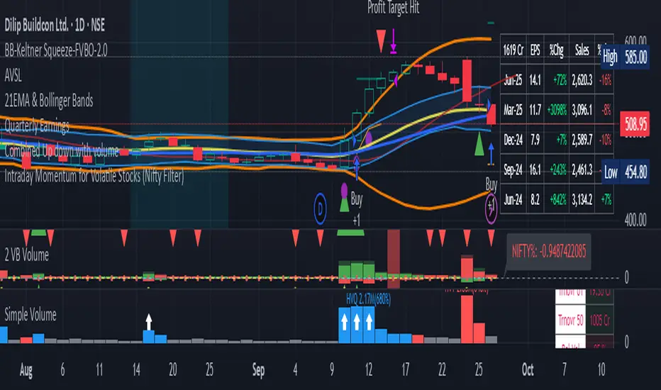
Intraday Momentum for Volatile Stocks 29.09The strategy targets intraday momentum breakouts in volatile stocks when the broader market (Nifty) is in an uptrend. It enters long positions when stocks move significantly above their daily opening price with sufficient volume confirmation, then manages the trade using dynamic ATR-based stops and profit targets.
Entry Conditions
Price Momentum Filter: The stock must move at least 2.5% above its daily opening price, indicating strong bullish momentum. This percentage threshold is customizable and targets gap-up scenarios or strong intraday breakouts.
Volume Confirmation: Daily cumulative volume must exceed the 20-day average volume, ensuring institutional participation and genuine momentum. This prevents false breakouts on low volume.
Market Regime Filter: The Nifty index must be trading above its 50-day SMA, indicating a favorable market environment for momentum trades. This macro filter helps avoid trades during bearish market conditions.
Money Flow Index: MFI must be above 50, confirming buying pressure and positive money flow into the stock. This adds another layer of momentum confirmation.
Time Restriction: Trades are only initiated before 3:00 PM to ensure sufficient time for position management and avoid end-of-day volatility.
Exit Management
ATR Trailing Stop Loss: Uses a 3x ATR multiplier for dynamic stop-loss placement that trails higher highs, protecting profits while giving trades room to breathe. The trailing mechanism locks in gains as the stock moves favorably.
Profit Target: Set at 4x ATR above the entry price, providing a favorable risk-reward ratio based on the stock's volatility characteristics. This adaptive approach adjusts targets based on individual stock behavior.
Position Reset: Both stops and targets reset when not in a position, ensuring fresh calculations for each new trade.
Key Strengths
Volatility Adaptation: The ATR-based approach automatically adjusts risk parameters to match current market volatility levels. Higher volatility stocks get wider stops, while calmer stocks get tighter management.
Multi-Timeframe Filtering: Combines intraday price action with daily volume patterns and market regime analysis for robust signal generation.
Risk Management Focus: The strategy prioritizes capital preservation through systematic stop-loss placement and position sizing considerations.
Considerations for NSE Trading
This strategy appears well-suited for NSE intraday momentum trading, particularly for mid-cap and small-cap stocks that exhibit high volatility. The Nifty filter helps align trades with broader market sentiment, which is crucial in the Indian market context where sectoral and index movements strongly influence individual stocks.
The 2.5% threshold above open price is appropriate for volatile NSE stocks, though traders might consider adjusting this parameter based on the specific stocks being traded. The strategy's emphasis on volume confirmation is particularly valuable in the NSE environment where retail participation can create misleading price movements without institutional backin
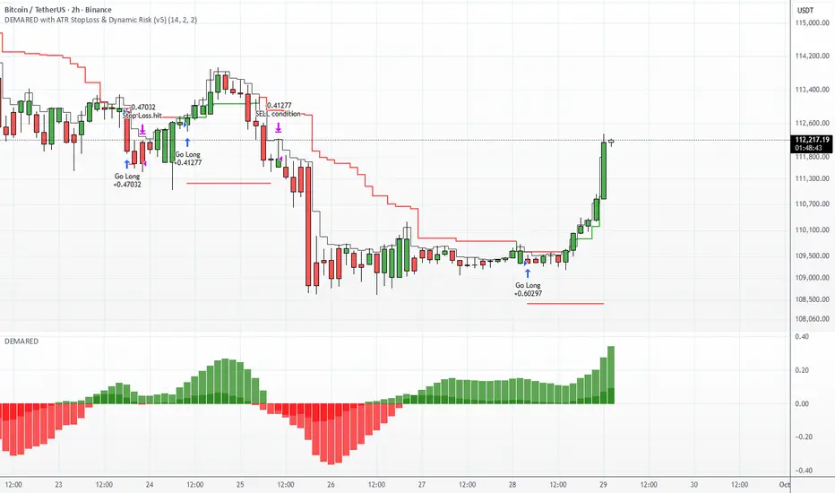
DEMARED with ATR StopLoss & Dynamic Risk (v5)DEMARED with ATR StopLoss & Dynamic Risk
This strategy combines Double Exponential Moving Averages (DEMA) with EMA and Donchian midline filters to capture trend-following signals. A long entry is triggered when both DEMA pairs are aligned bullishly, price is above EMA, and above the Donchian midpoint. Exits occur on opposite signals or when the ATR-based stop loss is hit.
Key features:
ATR Stop Loss: dynamic stop based on ATR with user-defined multiplier.
Dynamic Risk Management: position size is automatically calculated based on account equity and risk percentage.
Visualization: plots stop loss, EMA, Donchian midline, and optional bar coloring.
Flexible Display: toggle all indicator visuals on/off with a single input.
The goal is to provide a trend-following system with controlled risk and adaptability across different markets and timeframes.
Scalper's Dream by Chino,CHINO’S ICT MES/MNQ Strategy — FVG/BOS/OTE/PD + VWAP + SMA + BB Squeeze/Failure
Summary
Intraday ICT-inspired toolkit tuned for MES/MNQ (also effective on equities/ETFs and crypto). It blends Fair Value Gaps (FVG) — including multi-timeframe FVG (MTF FVG) with first-touch and min-gap filters — Break of Structure (BOS), Optimal Trade Entry (OTE), and Prior-Day levels with VWAP, SMA gates, 9:30 Open, Session Equilibrium (EQ), custom ORB, and Key Rejection Levels (KRL). It also includes Accumulation/Distribution phase reads and Manipulation cues (e.g., liquidity sweeps/stop-runs) to contextualize trend transitions. On top, it adds Bollinger Band squeeze breakouts & failure reversals, V/A shape reversal detectors, Volume-boosted buy/sell signals with Reversal Candle Assist, Asia/London/New York sessions, an Options Assist HUD, and a Market Internals HUD.
Disclaimer: This tool is for education and research purposes only and is not financial advice. Test thoroughly in replay/paper before live trading.
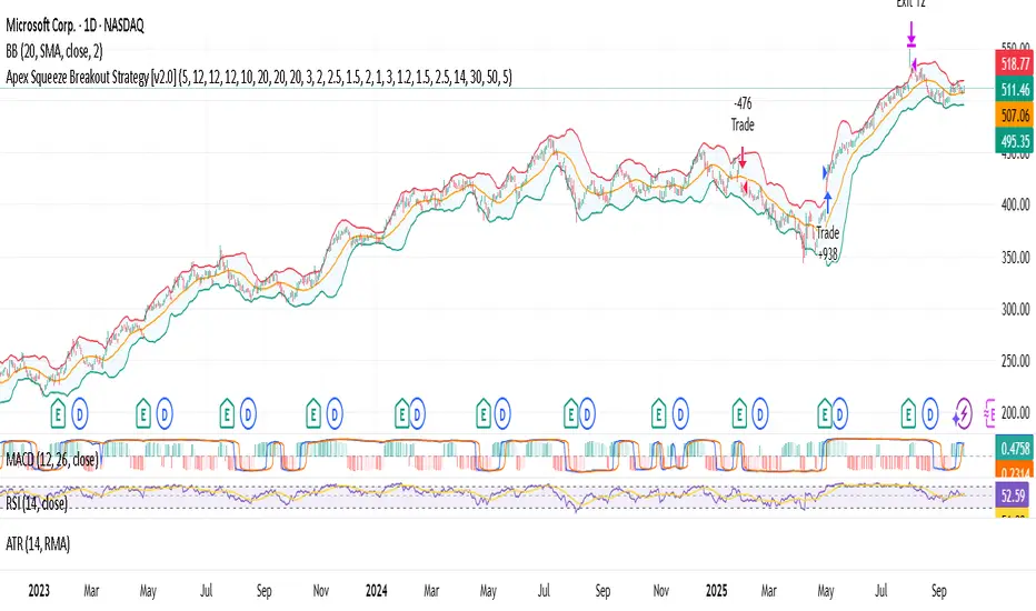
Apex Squeeze Breakout Strategy [by SKC]This is the official strategy version of the Apex Squeeze Breakout Trading System (v2.5 by SKC) indicator.
🔍 This script replicates the exact logic and trade behavior of the indicator, including:
Multi-factor scoring system (volume spike, squeeze, RSI recovery, momentum breakout, gap)
Supertrend-based trend bias and override logic
ATR-based dynamic SL/TP
Breakeven stop-loss shift after T1 hit
Trade logic works for both swing and day trading styles via a toggle
📈 Settings:
Use isDayTrading = true for 5m/15m charts
Use isDayTrading = false for 1H–Daily swing setups
⚠️ This strategy does not use repainting or offset entries. Backtest results are directly aligned with real-time signals from the original indicator.
✅ Use this strategy to backtest ticker performance, identify high-confidence symbols, and create forward trade plans based on proven edge.

简单KDJ80策略 - testIt's only a test of sth big.
Next step will be adding complex strategy with bollinger band and keltner channel.
Apex Squeeze Breakout Strategy (v1.0 by SKC)The Apex Squeeze Breakout Strategy is a powerful momentum-based system designed to capture explosive price moves following periods of low volatility compression (squeeze). It combines five key conditions to validate high-probability breakouts:
🔵 TTM Squeeze Detection using Bollinger Bands and Keltner Channels
🔊 Volume Spike Confirmation relative to a moving average
📈 Breakout Trigger above/below a recent high/low range
💪 Momentum Acceleration using percentage change over time
♻️ RSI Recovery / Overbought Logic to confirm shift in strength
The strategy includes:
Configurable swing/day trading modes
Dynamic ATR-based Stop Loss and TP1/TP2 system
Modular input structure for easy customization
Clear entry/exit visual markers and trade zones
It’s designed for disciplined traders who want to catch high-energy moves after consolidation, suitable for both intraday and swing setups.
RSI Momentum ScalperOverview
The "RSI Momentum Scalper" is a Pine Script v5 strategy crafted for trading highly volatile markets, with a special focus on newly listed cryptocurrencies. This strategy harnesses the Relative Strength Index (RSI) alongside volume analysis and momentum thresholds to pinpoint short-term trading opportunities. It supports both long and short trades, managed with customizable take profit, stop loss, and trailing stop levels, which are visually plotted on the chart for easy tracking.
Why I Created This Strategy
I developed the "RSI Momentum Scalper" because I was seeking a reliable trading strategy tailored to newly listed, highly volatile cryptocurrencies. These assets often experience rapid price fluctuations, rendering traditional strategies less effective. I aimed to create a tool that could exploit momentum and volume spikes while managing risk through adaptable exit parameters. This strategy is designed to address that need, offering a flexible approach for traders in dynamic crypto markets.
How It Works
The strategy utilizes RSI to identify momentum shifts, combined with volume confirmation, to trigger long or short entries. Trades are controlled with take profit, stop loss, and trailing stop levels, which adjust dynamically as the price moves in your favor. The trailing stop helps lock in profits, while the plotted exit levels provide clear visual cues for trade management.
Customizable Settings
The script is highly customizable, allowing you to adjust it to various market conditions and trading styles. Here’s a brief overview of the key settings:
Trade Mode: Select "Both," "Long Only," or "Short Only" to determine the trade direction.
(Default: Both)
RSI Length: Sets the lookback period for the RSI calculation (2 to 30).
(Default: 8)
A shorter length increases RSI sensitivity, suitable for volatile assets.
RSI Overbought: Defines the upper RSI threshold (60 to 99) for short entries.
(Default: 90)
Higher values signal stronger overbought conditions.
RSI Oversold: Defines the lower RSI threshold (1 to 40) for long entries.
(Default: 10)
Lower values indicate stronger oversold conditions.
RSI Momentum Threshold: Sets the minimum RSI momentum change (1 to 15) to trigger entries.
(Default: 14)
Adjusts the sensitivity to price momentum.
Volume Multiplier: Multiplies the volume moving average to filter high-volume bars (1.0 to 3.0).
(Default: 1)
Higher values require stronger volume confirmation.
Volume MA Length: Sets the lookback period for the volume moving average (5 to 50).
(Default: 13)
Influences the volume trend sensitivity.
Take Profit %: Sets the profit target as a percentage of the entry price (0.1 to 10.0).
(Default: 4.15)
Determines when to close a winning trade.
Stop Loss %: Sets the loss limit as a percentage of the entry price (0.1 to 6.0).
(Default: 1.85)
Protects against significant losses.
Trailing Stop %: Sets the trailing stop distance as a percentage (0.1 to 4.0).
(Default: 2.55)
Locks in profits as the price moves favorably.
Visual Features
Exit Levels: Take profit (green), fixed stop loss (red), and trailing stop (orange) levels are plotted when in a position.
Performance Table: Displays win rate, total trades, and net profit in the top-right corner.
How to Use
Add the strategy to your chart in TradingView.
Adjust the input settings based on the cryptocurrency and timeframe you’re trading.
Monitor the plotted exit levels for trade management.
Use the performance table to assess the strategy’s performance over time.
Notes
Test the strategy on a demo account or with historical data before live trading.
The strategy is optimized for short-term scalping; adjust settings for longer timeframes if needed.