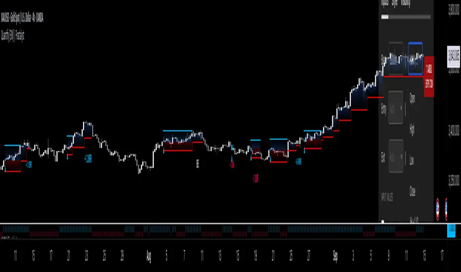
Quantify [Entry Model] | FractalystWhat’s the indicator’s purpose and functionality?
Quantify is a machine learning entry model designed to help traders identify high-probability setups to refine their strategies.
➙ Simply pick your bias, select your entry timeframes, and let Quantify handle the rest for you.
Can the indicator be applied to any market approach/trading strategy?
Absolutely, all trading strategies share one fundamental element: Directional Bias
Once you’ve determined the market bias using your own personal approach, whether it’s through technical analysis or fundamental analysis, select the trend direction in the Quantify user inputs.
The algorithm will then adjust its calculations to provide optimal entry levels aligned with your chosen bias. This involves analyzing historical patterns to identify setups with the highest potential expected values, ensuring your setups are aligned with the selected direction.
Can the indicator be used for different timeframes or trading styles?
Yes, regardless of the timeframe you’d like to take your entries, the indicator adapts to your trading style.
Whether you’re a swing trader, scalper, or even a position trader, the algorithm dynamically evaluates market conditions across your chosen timeframe.
How can this indicator help me to refine my trading strategy?
1. Focus on Positive Expected Value
• The indicator evaluates every setup to ensure it has a positive expected value, helping you focus only on trades that statistically favor long-term profitability.
2. Adapt to Market Conditions
• By analyzing real-time market behavior and historical patterns, the algorithm adjusts its calculations to match current conditions, keeping your strategy relevant and adaptable.
3. Eliminate Emotional Bias
• With clear probabilities, expected values, and data-driven insights, the indicator removes guesswork and helps you avoid emotional decisions that can damage your edge.
4. Optimize Entry Levels
• The indicator identifies optimal entry levels based on your selected bias and timeframes, improving robustness in your trades.
5. Enhance Risk Management
• Using tools like the Kelly Criterion, the indicator suggests optimal position sizes and risk levels, ensuring that your strategy maintains consistency and discipline.
6. Avoid Overtrading
• By highlighting only high-potential setups, the indicator keeps you focused on quality over quantity, helping you refine your strategy and avoid unnecessary losses.
How can I get started to use the indicator for my entries?
1. Set Your Market Bias
• Determine whether the market trend is Bullish or Bearish using your own approach.
• Select the corresponding bias in the indicator’s user inputs to align it with your analysis.
2. Choose Your Entry Timeframes
• Specify the timeframes you want to focus on for trade entries.
• The indicator will dynamically analyze these timeframes to provide optimal setups.
3. Let the Algorithm Analyze
• Quantify evaluates historical data and real-time price action to calculate probabilities and expected values.
• It highlights setups with the highest potential based on your selected bias and timeframes.
4. Refine Your Entries
• Use the insights provided—entry levels, probabilities, and risk calculations—to align your trades with a math-driven edge.
• Avoid overtrading by focusing only on setups with positive expected value.
5. Adapt to Market Conditions
• The indicator continuously adapts to real-time market behavior, ensuring its recommendations stay relevant and precise as conditions change.
How does the indicator calculate the current range?
The indicator calculates the current range by analyzing swing points from the very first bar on your charts to the latest available bar it identifies external liquidity levels, also known as BSLQ (buy-side liquidity levels) and SSLQ (sell-side liquidity levels).
What's the purpose of these levels? What are the underlying calculations?
1. Understanding Swing highs and Swing Lows
Swing High: A Swing High is formed when there is a high with 2 lower highs to the left and right.
Swing Low: A Swing Low is formed when there is a low with 2 higher lows to the left and right.
2. Understanding the purpose and the underlying calculations behind Buyside, Sellside and Pivot levels.
3. Identifying Discount and Premium Zones.
4. Importance of Risk-Reward in Premium and Discount Ranges
How does the script calculate probabilities?
The script calculates the probability of each liquidity level individually. Here's the breakdown:
1. Upon the formation of a new range, the script waits for the price to reach and tap into pivot level level. Status: "■" - Inactive
2. Once pivot level is tapped into, the pivot status becomes activated and it waits for either liquidity side to be hit. Status: "▶" - Active
3. If the buyside liquidity is hit, the script adds to the count of successful buyside liquidity occurrences. Similarly, if the sellside is tapped, it records successful sellside liquidity occurrences.
4. Finally, the number of successful occurrences for each side is divided by the overall count individually to calculate the range probabilities.
Note: The calculations are performed independently for each directional range. A range is considered bearish if the previous breakout was through a sellside liquidity. Conversely, a range is considered bullish if the most recent breakout was through a buyside liquidity.
What does the multi-timeframe functionality offer?
You can incorporate up to 4 higher timeframe probabilities directly into the table.
This feature allows you to analyze the probabilities of buyside and sellside liquidity across multiple timeframes, without the need to manually switch between them.
By viewing these higher timeframe probabilities in one place, traders can spot larger market trends and refine their entries and exits with a better understanding of the overall market context.
What are the multi-timeframe underlying calculations?
The script uses the same calculations (mentioned above) and uses security function to request the data such as price levels, bar time, probabilities and booleans from the user-input timeframe.
How does the Indicator Identifies Positive Expected Values?
Quantify instantly calculates whether a trade setup has the potential to generate positive expected value (EV).
To determine a positive EV setup, the indicator uses the formula:
EV = ( P(Win) × R(Win) ) − ( P(Loss) × R(Loss))
where:
- P(Win) is the probability of a winning trade.
- R(Win) is the reward or return for a winning trade, determined by the current risk-to-reward ratio (RR).
- P(Loss) is the probability of a losing trade.
- R(Loss) is the loss incurred per losing trade, typically assumed to be -1.
By calculating these values based on historical data and the current trading setup, the indicator helps you understand whether your trade has a positive expected value.
How can I know that the setup I'm going to trade with has a positive EV?
If the indicator detects that the adjusted pivot and buy/sell side probabilities have generated positive expected value (EV) in historical data, the risk-to-reward (RR) label within the range box will be colored blue and red .
If the setup does not produce positive EV, the RR label will appear gray.
This indicates that even the risk-to-reward ratio is greater than 1:1, the setup is not likely to yield a positive EV because, according to historical data, the number of losses outweighs the number of wins relative to the RR gain per winning trade.
What is the confidence level in the indicator, and how is it determined?
The confidence level in the indicator reflects the reliability of the probabilities calculated based on historical data. It is determined by the sample size of the probabilities used in the calculations. A larger sample size generally increases the confidence level, indicating that the probabilities are more reliable and consistent with past performance.
How does the confidence level affect the risk-to-reward (RR) label?
The confidence level (★) is visually represented alongside the probability label. A higher confidence level indicates that the probabilities used to determine the RR label are based on a larger and more reliable sample size.
How can traders use the confidence level to make better trading decisions?
Traders can use the confidence level to gauge the reliability of the probabilities and expected value (EV) calculations provided by the indicator. A confidence level above 95% is considered statistically significant and indicates that the historical data supporting the probabilities is robust. This high confidence level suggests that the probabilities are reliable and that the indicator’s recommendations are more likely to be accurate.
In data science and statistics, a confidence level above 95% generally means that there is less than a 5% chance that the observed results are due to random variation. This threshold is widely accepted in research and industry as a marker of statistical significance. Studies such as those published in the Journal of Statistical Software and the American Statistical Association support this threshold, emphasizing that a confidence level above 95% provides a strong assurance of data reliability and validity.
Conversely, a confidence level below 95% indicates that the sample size may be insufficient and that the data might be less reliable. In such cases, traders should approach the indicator’s recommendations with caution and consider additional factors or further analysis before making trading decisions.
How does the sample size affect the confidence level, and how does it relate to my TradingView plan?
The sample size for calculating the confidence level is directly influenced by the amount of historical data available on your charts. A larger sample size typically leads to more reliable probabilities and higher confidence levels.
Here’s how the TradingView plans affect your data access:
Essential Plan
The Essential Plan provides basic data access with a limited amount of historical data. This can lead to smaller sample sizes and lower confidence levels, which may weaken the robustness of your probability calculations. Suitable for casual traders who do not require extensive historical analysis.
Plus Plan
The Plus Plan offers more historical data than the Essential Plan, allowing for larger sample sizes and more accurate confidence levels. This enhancement improves the reliability of indicator calculations. This plan is ideal for more active traders looking to refine their strategies with better data.
Premium Plan
The Premium Plan grants access to extensive historical data, enabling the largest sample sizes and the highest confidence levels. This plan provides the most reliable data for accurate calculations, with up to 20,000 historical bars available for analysis. It is designed for serious traders who need comprehensive data for in-depth market analysis.
PRO+ Plans
The PRO+ Plans offer the most extensive historical data, allowing for the largest sample sizes and the highest confidence levels. These plans are tailored for professional traders who require advanced features and significant historical data to support their trading strategies effectively.
For many traders, the Premium Plan offers a good balance of affordability and sufficient sample size for accurate confidence levels.
What is the HTF probability table and how does it work?
The HTF (Higher Time Frame) probability table is a feature that allows you to view buy and sellside probabilities and their status from timeframes higher than your current chart timeframe.
Here’s how it works:
Data Request: The table requests and retrieves data from user-defined higher timeframes (HTFs) that you select.
Probability Display: It displays the buy and sellside probabilities for each of these HTFs, providing insights into the likelihood of price movements based on higher timeframe data.
Detailed Tooltips: The table includes detailed tooltips for each timeframe, offering additional context and explanations to help you understand the data better.
What do the different colors in the HTF probability table indicate?
The colors in the HTF probability table provide visual cues about the expected value (EV) of trading setups based on higher timeframe probabilities:
Blue: Suggests that entering a long position from the HTF user-defined pivot point, targeting buyside liquidity, is likely to result in a positive expected value (EV) based on historical data and sample size.
Red: Indicates that entering a short position from the HTF user-defined pivot point, targeting sellside liquidity, is likely to result in a positive expected value (EV) based on historical data and sample size.
Gray: Shows that neither long nor short trades from the HTF user-defined pivot point are expected to generate positive EV, suggesting that trading these setups may not be favorable.
What machine learning techniques are used in Quantify?
Quantify offers two main machine learning approaches:
1. Adaptive Learning (Fixed Sample Size): The algorithm learns from the entire dataset without resampling, maintaining a stable model that adapts to the latest market conditions.
2. Bootstrap Resampling: This method creates multiple subsets of the historical data, allowing the model to train on varying sample sizes. This technique enhances the robustness of predictions by ensuring that the model is not overfitting to a single dataset.
How does machine learning affect the expected value calculations in Quantify?
Machine learning plays a key role in improving the accuracy of expected value (EV) calculations. By analyzing historical price action, liquidity hits, and market bias patterns, the model continuously adjusts its understanding of risk and reward, allowing the expected value to reflect the most likely market movements. This results in more precise EV predictions, helping traders focus on setups that maximize profitability.
What is the Kelly Criterion, and how does it work in Quantify?
The Kelly Criterion is a mathematical formula used to determine the optimal position size for each trade, maximizing long-term growth while minimizing the risk of large drawdowns. It calculates the percentage of your portfolio to risk on a trade based on the probability of winning and the expected payoff.
Quantify integrates this with user-defined inputs to dynamically calculate the most effective position size in percentage, aligning with the trader’s risk tolerance and desired exposure.
How does Quantify use the Kelly Criterion in practice?
Quantify uses the Kelly Criterion to optimize position sizing based on the following factors:
1. Confidence Level: The model assesses the confidence level in the trade setup based on historical data and sample size. A higher confidence level increases the suggested position size because the trade has a higher probability of success.
2. Max Allowed Drawdown (User-Defined): Traders can set their preferred maximum allowed drawdown, which dictates how much loss is acceptable before reducing position size or stopping trading. Quantify uses this input to ensure that risk exposure aligns with the trader’s risk tolerance.
3. Probabilities: Quantify calculates the probabilities of success for each trade setup. The higher the probability of a successful trade (based on historical price action and liquidity levels), the larger the position size suggested by the Kelly Criterion.
What is a trailing stoploss, and how does it work in Quantify?
A trailing stoploss is a dynamic risk management tool that moves with the price as the market trend continues in the trader’s favor. Unlike a fixed take profit, which stays at a set level, the trailing stoploss automatically adjusts itself as the market moves, locking in profits as the price advances.
In Quantify, the trailing stoploss is enhanced by incorporating market structure liquidity levels (explain above). This ensures that the stoploss adjusts intelligently based on key price levels, allowing the trader to stay in the trade as long as the trend remains intact, while also protecting profits if the market reverses.
Why would a trader prefer a trailing stoploss based on liquidity levels instead of a fixed take-profit level?
Traders who use trailing stoplosses based on liquidity levels prefer this method because:
1. Market-Driven Flexibility: The stoploss follows the market structure rather than being static at a pre-defined level. This means the stoploss is less likely to be hit by small market fluctuations or false reversals. The stoploss remains adaptive, moving as the market moves.
2. Riding the Trend: Traders can capture more profit during a sustained trend because the trailing stop will adjust only when the trend starts to reverse significantly, based on key liquidity levels. This allows them to hold positions longer without prematurely locking in profits.
3. Avoiding Premature Exits: Fixed stoploss levels may exit a trade too early in volatile markets, while liquidity-based trailing stoploss levels respect the natural flow of price action, preventing the trader from exiting too soon during pullbacks or minor retracements.
🎲 Becoming the House: Gaining an Edge Over the Market
In American roulette, the casino has a 5.26% edge due to the presence of the 0 and 00 pockets. On even-money bets, players face a 47.37% chance of winning, while true 50/50 odds would require a 50% chance. This edge—the gap between the payout odds and the true probabilities—ensures that, statistically, the casino will always win over time, even if individual players win occasionally.
From a Trader’s Perspective
In trading, your edge comes from identifying and executing setups with a positive expected value (EV). For example:
• If you identify a setup with a 55.48% chance of winning and a 1:1 risk-to-reward (RR) ratio, your trade has a statistical advantage over a neutral (50/50) probability.
This edge works in your favor when applied consistently across a series of trades, just as the casino’s edge ensures profitability across thousands of spins.
🎰 Applying the Concept to Trading
Like casinos leverage their mathematical edge in games of chance, you can achieve long-term success in trading by focusing on setups with positive EV and managing your trades systematically. Here’s how:
1. Probability Advantage: Prioritize trades where the probability of success (win rate) exceeds the breakeven rate for your chosen risk-to-reward ratio.
• Example: With a 1:1 RR, you need a win rate above 50% to achieve positive EV.
2. Risk-to-Reward Ratio (RR): Even with a win rate below 50%, you can gain an edge by increasing your RR (e.g., a 40% win rate with a 2:1 RR still has positive EV).
3. Consistency and Discipline: Just as casinos profit by sticking to their mathematical advantage over thousands of spins, traders must rely on their edge across many trades, avoiding emotional decisions or overleveraging.
By targeting favorable probabilities and managing trades effectively, you “become the house” in your trading. This approach allows you to leverage statistical advantages to enhance your overall performance and achieve sustainable profitability.
What Makes the Quantify Indicator Original?
1. Data-Driven Edge
Unlike traditional indicators that rely on static formulas, Quantify leverages probability-based analysis and machine learning. It calculates expected value (EV) and confidence levels to help traders identify setups with a true statistical edge.
2. Integration of Market Structure
Quantify uses market structure liquidity levels to dynamically adapt. It identifies key zones like swing highs/lows and liquidity traps, enabling users to align entries and exits with where the market is most likely to react. This bridges the gap between price action analysis and quantitative trading.
3. Sophisticated Risk Management
The Kelly Criterion implementation is unique. Quantify allows traders to input their maximum allowed drawdown, dynamically adjusting risk exposure to maintain optimal position sizing. This ensures risk is scientifically controlled while maximizing potential growth.
4. Multi-Timeframe and Liquidity-Based Trailing Stops
The indicator doesn’t just suggest fixed profit-taking levels. It offers market structure-based trailing stop-loss functionality, letting traders ride trends as long as liquidity and probabilities favor the position, which is rare in most tools.
5. Customizable Bias and Adaptive Learning
• Directional Bias: Traders can set a bullish or bearish bias, and the indicator recalculates probabilities to align with the trader’s market outlook.
• Adaptive Learning: The machine learning model adapts to changes in data (via resampling or bootstrap methods), ensuring that predictions stay relevant in evolving markets.
6. Positive EV Focus
The focus on positive EV setups differentiates it from reactive indicators. It shifts trading from chasing signals to acting on setups that statistically favor profitability, akin to how professional quant funds operate.
7. User Empowerment
Through features like customizable timeframes, real-time probability updates, and visualization tools, Quantify empowers users to make data-informed decisions.
Terms and Conditions | Disclaimer
Our charting tools are provided for informational and educational purposes only and should not be construed as financial, investment, or trading advice. They are not intended to forecast market movements or offer specific recommendations. Users should understand that past performance does not guarantee future results and should not base financial decisions solely on historical data.
Built-in components, features, and functionalities of our charting tools are the intellectual property of @Fractalyst use, reproduction, or distribution of these proprietary elements is prohibited.
By continuing to use our charting tools, the user acknowledges and accepts the Terms and Conditions outlined in this legal disclaimer and agrees to respect our intellectual property rights and comply with all applicable laws and regulations.
Probability
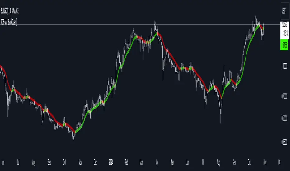
PDF Smoothed Moving Average [BackQuant]PDF Smoothed Moving Average
Introducing BackQuant’s PDF Smoothed Moving Average (PDF-MA) — an innovative trading indicator that applies Probability Density Function (PDF) weighting to moving averages, creating a unique, trend-following tool that offers adaptive smoothing to price movements. This advanced indicator gives traders an edge by blending PDF-weighted values with conventional moving averages, helping to capture trend shifts with enhanced clarity.
Core Concept: Probability Density Function (PDF) Smoothing
The Probability Density Function (PDF) provides a mathematical approach to applying adaptive weighting to data points based on a specified variance and mean. In the PDF-MA indicator, the PDF function is used to weight price data, adding a layer of probabilistic smoothing that enhances the detection of trend strength while reducing noise.
The PDF weights are controlled by two key parameters:
Variance: Determines the spread of the weights, where higher values spread out the weighting effect, providing broader smoothing.
Mean : Centers the weights around a particular price value, influencing the trend’s directionality and sensitivity.
These PDF weights are applied to each price point over the chosen period, creating an adaptive and smooth moving average that more closely reflects the underlying price trend.
Blending PDF with Standard Moving Averages
To further improve the PDF-MA, this indicator combines the PDF-weighted average with a traditional moving average, selected by the user as either an Exponential Moving Average (EMA) or Simple Moving Average (SMA). This blended approach leverages the strengths of each method: the responsiveness of PDF smoothing and the robustness of conventional moving averages.
Smoothing Method: Traders can choose between EMA and SMA for the additional moving average layer. The EMA is more responsive to recent prices, while the SMA provides a consistent average across the selected period.
Smoothing Period: Controls the length of the lookback period, affecting how sensitive the average is to price changes.
The result is a PDF-MA that provides a reliable trend line, reflecting both the PDF weighting and traditional moving average values, ideal for use in trend-following and momentum-based strategies.
Trend Detection and Candle Coloring
The PDF-MA includes a built-in trend detection feature that dynamically colors candles based on the direction of the smoothed moving average:
Uptrend: When the PDF-MA value is increasing, the trend is considered bullish, and candles are colored green, indicating potential buying conditions.
Downtrend: When the PDF-MA value is decreasing, the trend is considered bearish, and candles are colored red, signaling potential selling or shorting conditions.
These color-coded candles provide a quick visual reference for the trend direction, helping traders make real-time decisions based on the current market trend.
Customization and Visualization Options
This indicator offers a range of customization options, allowing traders to tailor it to their specific preferences and trading environment:
Price Source : Choose the price data for calculation, with options like close, open, high, low, or HLC3.
Variance and Mean : Fine-tune the PDF weighting parameters to control the indicator’s sensitivity and responsiveness to price data.
Smoothing Method : Select either EMA or SMA to customize the conventional moving average layer used in conjunction with the PDF.
Smoothing Period : Set the lookback period for the moving average, with a longer period providing more stability and a shorter period offering greater sensitivity.
Candle Coloring : Enable or disable candle coloring based on trend direction, providing additional clarity in identifying bullish and bearish phases.
Trading Applications
The PDF Smoothed Moving Average can be applied across various trading strategies and timeframes:
Trend Following : By smoothing price data with PDF weighting, this indicator helps traders identify long-term trends while filtering out short-term noise.
Reversal Trading : The PDF-MA’s trend coloring feature can help pinpoint potential reversal points by showing shifts in the trend direction, allowing traders to enter or exit positions at optimal moments.
Swing Trading : The PDF-MA provides a clear trend line that swing traders can use to capture intermediate price moves, following the trend direction until it shifts.
Final Thoughts
The PDF Smoothed Moving Average is a highly adaptable indicator that combines probabilistic smoothing with traditional moving averages, providing a nuanced view of market trends. By integrating PDF-based weighting with the flexibility of EMA or SMA smoothing, this indicator offers traders an advanced tool for trend analysis that adapts to changing market conditions with reduced lag and increased accuracy.
Whether you’re trading trends, reversals, or swings, the PDF-MA offers valuable insights into the direction and strength of price movements, making it a versatile addition to any trading strategy.
AutoPilot | FractalystWhat’s the purpose of this indicator?
The AutoPilot indicator automates the management of your active trades by:
Breaks Even: Moves the stop-loss to the entry price once the trade reaches a 1:1 risk-reward ratio.
Closes Trades: Automatically exits trades when trailing stop-losses are triggered.
This automation is facilitated through PineConnector and TradingView webhook integration, allowing traders to manage multiple positions across various markets effortlessly without any manual intervention.
----
How does this indicator trail stop-loss using market structure?
The AutoPilot indicator utilizes an advanced market structure trailing stop-loss mechanism to manage trades based on market dynamics and probabilities.
Here's how it works:
Market Structure Identification: The indicator first identifies key market structures such as higher highs, lower lows.
These structures are pivotal points where the market has shown a change in direction or momentum.
Probability-Based Trailing: Once a trade is active, the stop-loss isn't just set at a fixed distance or percentage but is dynamically adjusted based on the probability of the market structure holding or breaking.
This involves:
Trend Continuation Probability: If the market structure suggests a strong trend continuation (e.g., a series of higher highs in an uptrend), the stop-loss might trail closer to the price, but with a buffer calculated by the probability of the trend continuing versus reversing.
Reversal Probability: Conversely, if there's a high probability of a trend reversal based on recent market structures (like a significant lower high in an uptrend), the stop-loss might be adjusted to a point where the market structure would need to break to confirm the reversal, thus protecting potential profits or minimizing losses.
Dynamic Adjustment: The trailing stop-loss adjusts in real-time as new market structures form. For instance, if a new higher high is formed in an uptrend, the stop-loss might move up but not necessarily to the exact previous swing low. Instead, it's placed at a level where the probability of the next swing low not breaking this level is high, based on historical price action.
Risk Management: By using market structure and probabilities, the indicator aims to balance between giving the trade room to breathe (allowing for normal market fluctuations) and tightening the stop-loss when the market behavior suggests a potential trend change or continuation with high confidence.
This approach ensures that the stop-loss isn't just a static or simple trailing mechanism but a sophisticated tool that adapts to the evolving market conditions, aiming to maximize profit while minimizing the risk of being stopped out prematurely due to market noise.
----
How are the probabilities calculated? What are the underlying calculations?
The probability is designed to enhance trade management by using buyside liquidity and probability analysis to filter out low/high probability conditions.
This helps in identifying optimal trailing points where the likelihood of a price continuation is higher.
Calculations:
1. Understanding Swing highs and Swing Lows
Swing High: A Swing High is formed when there is a high with 2 lower highs to the left and right.
Swing Low: A Swing Low is formed when there is a low with 2 higher lows to the left and right.
2. Understanding the purpose and the underlying calculations behind Buyside, Sellside and Equilibrium levels.
3. Understanding probability calculations
1. Upon the formation of a new range, the script waits for the price to reach and tap into equilibrium or the 50% level. Status: "⏸" - Inactive
2. Once equilibrium is tapped into, the equilibrium status becomes activated and it waits for either liquidity side to be hit. Status: "▶" - Active
3. If the buyside liquidity is hit, the script adds to the count of successful buyside liquidity occurrences. Similarly, if the sellside is tapped, it records successful sellside liquidity occurrences.
5. Finally, the number of successful occurrences for each side is divided by the overall count individually to calculate the range probabilities.
Note: The calculations are performed independently for each directional range. A range is considered bearish if the previous breakout was through a sellside liquidity. Conversely, a range is considered bullish if the most recent breakout was through a buyside liquidity.
----
What does the automation table display?
The automation table in the AutoPilot indicator provides a summary of user-defined settings crucial for automated trade management through PineConnector and TradingView integration. It displays:
PineConnector License ID: This ensures that the indicator is linked to your specific PineConnector account, allowing for personalized and secure automation of your trades.
Order Type (Buy/Sell): Indicates whether the automation is set for buying or selling, which is essential for correctly executing your trading strategy.
Chosen Symbol: Specifies the trading pair or symbol in your broker's platform where the trade management commands (like closing orders) will be executed. This ensures that the automation targets the correct market or asset.
Risk Per Trade: Shows the percentage or amount of your capital you're willing to risk on each trade, helping you maintain consistent risk management across different trades.
Comment: A field for you to input notes or identifiers, particularly useful when trading across multiple markets or instruments. This helps in tracking and managing trades across different assets or strategies.
Comment: A field for you to input identifiers, particularly useful when trading across multiple timeframes or different enries.
Allowing users to manage specific comments for each previously taken entry, facilitating precise management of multiple trades with unique identifiers.
This table serves as a quick reference for your current settings, ensuring you're always aware of how your trades are being managed automatically before any adjustments are made or alerts are triggered.
----
How to use the indicator?
To use the AutoPilot indicator:
Purchase a License ID: Acquire a license ID from PineConnector.
Setup PineConnector EA: Install and configure the PineConnector Expert Advisor on your MetaTrader platform.
Input Settings: Enter your PineConnector license ID, choose the order type, set your risk per trade, add the order comment, and select the trading symbol in the indicator's settings.
Create Alert: Right-click on the automation table, and set up an alert with the provided webhook to connect with PineConnector.
Automatic Management: Once set, your active trades will be automatically managed according to the alert conditions you've set.
This setup ensures your trades are managed seamlessly without constant manual intervention.
----
What makes this indicator original?
Integration with PineConnector: The AutoPilot indicator's originality lies in its integration with PineConnector, which allows for real-time trade management directly from TradingView to your MetaTrader platform. This setup is unique as it combines the analytical capabilities of TradingView with the execution capabilities of MetaTrader through a custom indicator, providing a seamless bridge between analysis and action.
Market Structure-Based Trailing Stop-Loss: Unlike many indicators that might use fixed percentages or ATR (Average True Range) for stop-loss adjustments, the AutoPilot indicator uses market structure (higher highs, lower lows) to dynamically adjust the stop-loss.
Probability-Based Adjustments: The indicator doesn't just trail stop-losses based on price but incorporates the probability of market structure holding or breaking. This probability-based trailing mechanism is innovative, aiming to balance between giving trades room to breathe and tightening when market behavior suggests a potential reversal or continuation.
Customizable Automation Table: The automation table within the indicator allows for detailed customization, including setting specific comments for trades. This feature, while perhaps not unique in concept, is original in its implementation within trading indicators, providing users with a high degree of control and personalization over trade management.
Real-Time Trade Management Alerts: The ability to set up alerts directly from the indicator to manage trades in real-time via webhooks to PineConnector adds a layer of automation that's not commonly found in standard trading indicators. This real-time connection for trade management enhances its originality by reducing the lag between analysis and trade execution.
User-Centric Design: The design of the AutoPilot indicator focuses heavily on user interaction, allowing for inputs like risk per trade, specific order types, and comments. This user-centric approach, where the indicator adapts to the trader's strategy rather than the trader adapting to the tool, sets it apart.
External Integration for Enhanced Functionality: By leveraging external services like PineConnector for execution, the indicator extends its functionality beyond what's typically possible within TradingView alone, making it original in its ecosystem integration for trading purposes.
Practical Implication: This means if you're in a trade and the market structure suggests the trend is continuing (e.g., making higher highs in an uptrend), your stop-loss might trail closer to the price but not too close to avoid being stopped out by normal fluctuations. If the structure breaks (e.g., a lower high in an uptrend), the stop-loss could adjust more aggressively to protect profits or minimize losses, anticipating a potential trend change.
This combination of features creates an original tool that not only analyzes market conditions but actively manages trades based on sophisticated market structure analysis.
----
User-input settings and customizations
----
Terms and Conditions | Disclaimer
Our charting tools are provided for informational and educational purposes only and should not be construed as financial, investment, or trading advice. They are not intended to forecast market movements or offer specific recommendations. Users should understand that past performance does not guarantee future results and should not base financial decisions solely on historical data. By utilizing our charting tools, the buyer acknowledges that neither the seller nor the creator assumes responsibility for decisions made using the information provided. The buyer assumes full responsibility and liability for any actions taken and their consequences, including potential financial losses. Therefore, by purchasing these charting tools, the customer acknowledges that neither the seller nor the creator is liable for any unfavorable outcomes resulting from the development, sale, or use of the products.
The buyer is responsible for canceling their subscription if they no longer wish to continue at the full retail price. Our policy does not include reimbursement, refunds, or chargebacks once the Terms and Conditions are accepted before purchase.
By continuing to use our charting tools, the user acknowledges and accepts the Terms and Conditions outlined in this legal disclaimer.

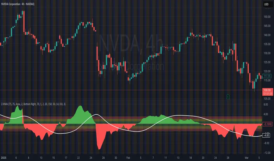
HMA Z-Score Probability Indicator by Erika BarkerThis indicator is a modified version of SteverSteves's original work, enhanced by Erika Barker. It visually represents asset price movements in terms of standard deviations from a Hull Moving Average (HMA), commonly known as a Z-Score.
Key Features:
Z-Score Calculation: Measures how many standard deviations the current price is from its HMA.
Hull Moving Average (HMA): This moving average provides a more responsive baseline for Z-Score calculations.
Flexible Display: Offers both area and candlestick visualization options for the Z-Score.
Probability Zones: Color-coded areas showing the statistical likelihood of prices based on their Z-Score.
Dynamic Price Level Labels: Displays actual price levels corresponding to Z-Score values.
Z-Table: An optional table showing the probability of occurrence for different Z-Score ranges.
Standard Deviation Lines: Horizontal lines at each standard deviation level for easy reference.
How It Works:
The indicator calculates the Z-Score by comparing the current price to its HMA and dividing by the standard deviation. This Z-Score is then plotted on a separate pane below the main chart.
Green areas/candles: Indicate prices above the HMA (positive Z-Score)
Red areas/candles: Indicate prices below the HMA (negative Z-Score)
Color-coded zones:
Green: Within 1 standard deviation (high probability)
Yellow: Between 1 and 2 standard deviations (medium probability)
Red: Beyond 2 standard deviations (low probability)
The HMA line (white) shows the trend of the Z-Score itself, offering insight into whether the asset is becoming more or less volatile over time.
Customization Options:
Adjust lookback periods for Z-Score and HMA calculations
Toggle between area and candlestick display
Show/hide probability fills, Z-Table, HMA line, and standard deviation bands
Customize text color and decimal rounding for price levels
Interpretation:
This indicator helps traders identify potential overbought or oversold conditions based on statistical probabilities. Extreme Z-Score values (beyond ±2 or ±3) often suggest a higher likelihood of mean reversion, while consistent Z-Scores in one direction may indicate a strong trend.
By combining the Z-Score with the HMA and probability zones, traders can gain a nuanced understanding of price movements relative to recent trends and their statistical significance.
Price Close ProbabilityThe Price Close Probability Indicator is designed to help traders estimate the likelihood of price closing above or below specified levels within a given bar. By placing two levels on your chart, you can quickly gauge the probability of the current price bar closing above or below these levels in real-time.
Key Features:
Dynamic Probability Calculation: The indicator continuously updates the probability of price closing above or below your set levels as the current bar progresses, providing you with timely insights as the bar approaches its close.
Customizable Standard Deviation : Adjust the length of the Standard Deviation used in the calculations to tailor the probability estimates to your preferred settings.
User-Friendly Probability Table : A clean, easy-to-read table displays the calculated probabilities, helping you make informed trading decisions at a glance.
Assumptions and Considerations:
While the indicator assumes that returns are normally distributed, which may not fully reflect reality, it still offers a valuable approximation of the probabilities for price movement within the current bar.
Future Enhancements (Coming Soon):
Multi-Bar Probability: Calculate probabilities across multiple bars to enhance your forecasting capabilities.
Additional Levels: Set more than two levels for a broader analysis of price movements.
Refined Distribution Modeling: Improve the accuracy of probability calculations by adjusting for more realistic return distributions.
Disclaimer
Please remember that past performance may not be indicative of future results.
Due to various factors, including changing market conditions, the strategy may no longer perform as well as in historical backtesting.
This post and the script don’t provide any financial advice.

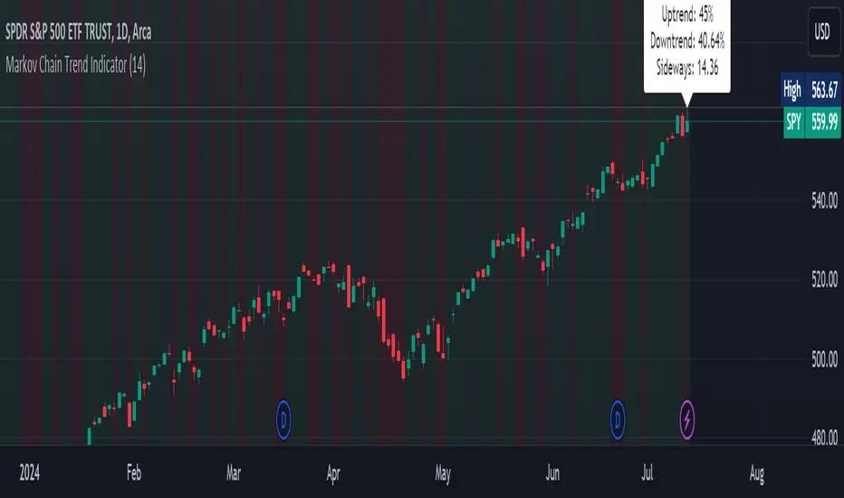
Markov Chain Trend IndicatorOverview
The Markov Chain Trend Indicator utilizes the principles of Markov Chain processes to analyze stock price movements and predict future trends. By calculating the probabilities of transitioning between different market states (Uptrend, Downtrend, and Sideways), this indicator provides traders with valuable insights into market dynamics.
Key Features
State Identification: Differentiates between Uptrend, Downtrend, and Sideways states based on price movements.
Transition Probability Calculation: Calculates the probability of transitioning from one state to another using historical data.
Real-time Dashboard: Displays the probabilities of each state on the chart, helping traders make informed decisions.
Background Color Coding: Visually represents the current market state with background colors for easy interpretation.
Concepts Underlying the Calculations
Markov Chains: A stochastic process where the probability of moving to the next state depends only on the current state, not on the sequence of events that preceded it.
Logarithmic Returns: Used to normalize price changes and identify states based on significant movements.
Transition Matrices: Utilized to store and calculate the probabilities of moving from one state to another.
How It Works
The indicator first calculates the logarithmic returns of the stock price to identify significant movements. Based on these returns, it determines the current state (Uptrend, Downtrend, or Sideways). It then updates the transition matrices to keep track of how often the price moves from one state to another. Using these matrices, the indicator calculates the probabilities of transitioning to each state and displays this information on the chart.
How Traders Can Use It
Traders can use the Markov Chain Trend Indicator to:
Identify Market Trends: Quickly determine if the market is in an uptrend, downtrend, or sideways state.
Predict Future Movements: Use the transition probabilities to forecast potential market movements and make informed trading decisions.
Enhance Trading Strategies: Combine with other technical indicators to refine entry and exit points based on predicted trends.
Example Usage Instructions
Add the Markov Chain Trend Indicator to your TradingView chart.
Observe the background color to quickly identify the current market state:
Green for Uptrend, Red for Downtrend, Gray for Sideways
Check the dashboard label to see the probabilities of transitioning to each state.
Use these probabilities to anticipate market movements and adjust your trading strategy accordingly.
Combine the indicator with other technical analysis tools for more robust decision-making.
Introducing the Markov Chain Model IndicatorThis powerful tool leverages Markov chain theory to help traders predict stock price movements by analyzing historical price data and calculating transition probabilities between different states: "Up by >1%", "Stable", and "Down by <1%". This post will provide a comprehensive overview of the indicator, its advantages and disadvantages, and how it can be used effectively in trading decisions.
How It Works
The Markov Chain Model indicator calculates the daily percentage changes in stock prices and categorizes them into three states:
Up by >1%
Stable (between -1% and +1%)
Down by <1%
By analyzing these transitions, the script constructs a transition matrix that shows the probability of moving from one state to another. This matrix is then displayed on the chart, providing traders with valuable insights into potential future price movements.
Advantages of the Markov Chain Model Indicator
Data-Driven Predictions : Utilizes historical price data to calculate probabilities, offering a statistical foundation for predictions.
Visual Representation : Displays the transition matrix directly on the chart, making it easy to interpret and use in trading decisions.
Adaptability : Allows users to customize the percentage threshold, enabling fine-tuning based on different market conditions.
Comprehensive Analysis : Considers multiple states (up, stable, down), providing a more nuanced view of price movements.
Disadvantages of the Markov Chain Model Indicator
Historical Dependence : The model relies on historical data, which may not always accurately predict future movements, especially in volatile markets.
Simplified States : The use of only three states might oversimplify complex market behaviors, potentially missing out on subtler trends.
Limited Scope : Designed for short-term predictions and may not be as effective for long-term investment strategies.
Example Interpretation
Transition Matrix:
From/To | Up >1% | Stable | Down <1% |
---------------------------------------
Up >1% | 0.30 | 0.40 | 0.30 |
Stable | 0.33 | 0.44 | 0.23 |
Down <1% | 0.34 | 0.36 | 0.30 |
Latest 3 States: S2 -> S1 -> S1
Total Bars: 2523
Decision Making Based on the Transition Matrix:
Current State: Up >1%
Next State Probabilities : 30% Up >1%, 40% Stable, 30% Down <1%
Decision : Given the balanced probabilities, a trader might decide to hold the position but set a trailing stop-loss to protect against sudden downturns. If other technical indicators also suggest continued upward momentum, they might increase their position cautiously.
Current State : Stable
Next State Probabilities : 33% Up >1%, 44% Stable, 23% Down <1%
Decision : With a high probability of stability, a cautious approach might be to hold or make small incremental trades, keeping an eye on other market indicators for confirmation.
Conclusion
The Markov Chain Model indicator is a powerful tool for traders looking to leverage statistical models to predict stock price movements. By understanding the transition probabilities between different states, traders can make more informed decisions and better manage their risk. We hope this tool helps enhance your trading strategy and provides you with a deeper understanding of market behaviors.
Try It Out
Copy the script above into TradingView and start exploring the potential of the Markov Chain Model indicator. Happy trading!
Feel free to share your feedback and let us know how this indicator works for you. Your insights can help us improve and develop even more effective trading tools.

Bayesian Trend Indicator [ChartPrime]Bayesian Trend Indicator
Overview:
In probability theory and statistics, Bayes' theorem (alternatively Bayes' law or Bayes' rule), named after Thomas Bayes, describes the probability of an event, based on prior knowledge of conditions that might be related to the event.
The "Bayesian Trend Indicator" is a sophisticated technical analysis tool designed to assess the direction of price trends in financial markets. It combines the principles of Bayesian probability theory with moving average analysis to provide traders with a comprehensive understanding of market sentiment and potential trend reversals.
At its core, the indicator utilizes multiple moving averages, including the Exponential Moving Average (EMA), Simple Moving Average (SMA), Double Exponential Moving Average (DEMA), and Volume Weighted Moving Average (VWMA) . These moving averages are calculated based on user-defined parameters such as length and gap length, allowing traders to customize the indicator to suit their trading strategies and preferences.
The indicator begins by calculating the trend for both fast and slow moving averages using a Smoothed Gradient Signal Function. This function assigns a numerical value to each data point based on its relationship with historical data, indicating the strength and direction of the trend.
// Smoothed Gradient Signal Function
sig(float src, gap)=>
ta.ema(source >= src ? 1 :
source >= src ? 0.9 :
source >= src ? 0.8 :
source >= src ? 0.7 :
source >= src ? 0.6 :
source >= src ? 0.5 :
source >= src ? 0.4 :
source >= src ? 0.3 :
source >= src ? 0.2 :
source >= src ? 0.1 :
0, 4)
Next, the indicator calculates prior probabilities using the trend information from the slow moving averages and likelihood probabilities using the trend information from the fast moving averages . These probabilities represent the likelihood of an uptrend or downtrend based on historical data.
// Define prior probabilities using moving averages
prior_up = (ema_trend + sma_trend + dema_trend + vwma_trend) / 4
prior_down = 1 - prior_up
// Define likelihoods using faster moving averages
likelihood_up = (ema_trend_fast + sma_trend_fast + dema_trend_fast + vwma_trend_fast) / 4
likelihood_down = 1 - likelihood_up
Using Bayes' theorem , the indicator then combines the prior and likelihood probabilities to calculate posterior probabilities, which reflect the updated probability of an uptrend or downtrend given the current market conditions. These posterior probabilities serve as a key signal for traders, informing them about the prevailing market sentiment and potential trend reversals.
// Calculate posterior probabilities using Bayes' theorem
posterior_up = prior_up * likelihood_up
/
(prior_up * likelihood_up + prior_down * likelihood_down)
Key Features:
◆ The trend direction:
To visually represent the trend direction , the indicator colors the bars on the chart based on the posterior probabilities. Bars are colored green to indicate an uptrend when the posterior probability is greater than 0.5 (>50%), while bars are colored red to indicate a downtrend when the posterior probability is less than 0.5 (<50%).
◆ Dashboard on the chart
Additionally, the indicator displays a dashboard on the chart , providing traders with detailed information about the probability of an uptrend , as well as the trends for each type of moving average. This dashboard serves as a valuable reference for traders to monitor trend strength and make informed trading decisions.
◆ Probability labels and signals:
Furthermore, the indicator includes probability labels and signals , which are displayed near the corresponding bars on the chart. These labels indicate the posterior probability of a trend, while small diamonds above or below bars indicate crossover or crossunder events when the posterior probability crosses the 0.5 threshold (50%).
The posterior probability of a trend
Crossover or Crossunder events
◆ User Inputs
Source:
Description: Defines the price source for the indicator's calculations. Users can select between different price values like close, open, high, low, etc.
MA's Length:
Description: Sets the length for the moving averages used in the trend calculations. A larger length will smooth out the moving averages, making the indicator less sensitive to short-term fluctuations.
Gap Length Between Fast and Slow MA's:
Description: Determines the difference in lengths between the slow and fast moving averages. A higher gap length will increase the difference, potentially identifying stronger trend signals.
Gap Signals:
Description: Defines the gap used for the smoothed gradient signal function. This parameter affects the sensitivity of the trend signals by setting the number of bars used in the signal calculations.
In summary, the "Bayesian Trend Indicator" is a powerful tool that leverages Bayesian probability theory and moving average analysis to help traders identify trend direction, assess market sentiment, and make informed trading decisions in various financial markets.

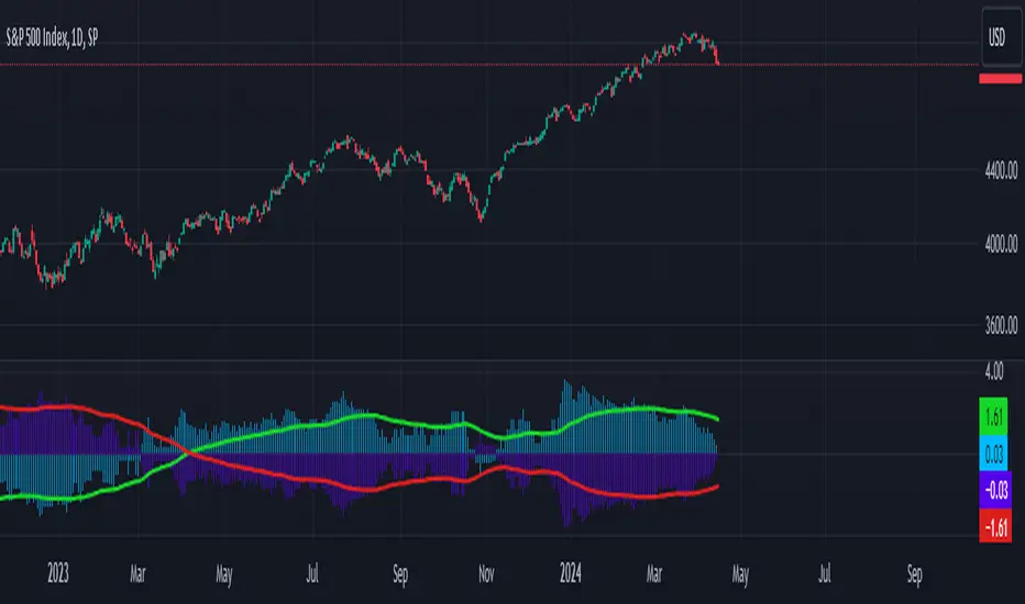
Bayesian Bias OscillatorWhat is a Bayes Estimator?
Bayesian estimation, or Bayesian inference, is a statistical method for estimating unknown parameters of a probability distribution based on observed data and prior knowledge about those parameters. At first , you will need a prior probability distribution, which is a prior belief about the distribution of the parameter that you are interested in estimating. This distribution represents your initial beliefs or knowledge about the parameter value before observing any data. Second , you need a likelihood function, which represents the probability of observing the data given different values of the parameter. This function quantifies how well different parameter values explain the observed data. Then , you will need a posterior probability distribution by combining the prior distribution and the likelihood function to obtain the posterior distribution of the parameter. The posterior distribution represents the updated belief about the parameter value after observing the data.
Bayesian Bias Oscillator
This tool calculates the Bayes bias of returns, which are directional probabilities that provide insight on the "trend" of the market or the directional bias of returns. It comes with two outputs: the default one, which is the Z-Score of the Bayes Bias, and the regular raw probability, which can be switched on in the settings of the indicator.
The Z-Score output value doesn't tell you the probability, but it does tell you how much of a standard deviation the value is from the mean. It uses both probabilities, the probability of a positive return and the probability of a negative return, which is just (1 - probability of a positive return).
The probability output value shows you the raw probability of a positive return vs. the probability of a negative return. The probability is the value of each line plotted (blue is the probability of a positive return, and purple is the probability of a negative return).
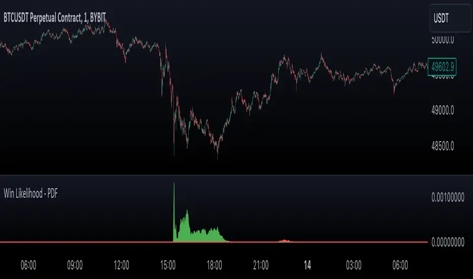
Likelihood of Winning - Probability Density FunctionIn developing the "Likelihood of Winning - Probability Density Function (PDF)" indicator, my aim was to offer traders a statistical tool to quantify the probability of reaching target prices. This indicator, grounded in risk assessment principles, enables users to analyze potential outcomes based on the normal distribution, providing insights into market dynamics.
The tool's flexibility allows for customization of the data series, lookback periods, and target settings for both long and short scenarios. It features a color-coded visualization to easily distinguish between probabilities of hitting specified targets, enhancing decision-making in trading strategies.
I'm excited to share this indicator with the trading community, hoping it will enhance data-driven decision-making and offer a deeper understanding of market risks and opportunities. My goal is to continuously improve this tool based on user feedback and market evolution, contributing to more informed trading practices.
This indicator leverages the "NormalDistributionFunctions" library, enabling easy integration into other indicators or strategies. Users can readily embed advanced statistical analysis into their trading tools, fostering innovation within the Pine Script community.
Breakout Probability Indicator (FinnoVent)The Breakout Probability Indicator is a cutting-edge tool designed for traders looking to gauge the likelihood of price breakouts above or below current levels. This indicator intelligently combines Average True Range (ATR) and recent price action to provide a probabilistic insight into potential future price movements, enhancing strategy formulation and risk management.
Core Features:
Volatility Assessment: Utilizes the Average True Range (ATR) to measure market volatility, a critical component in identifying potential breakout scenarios.
Dynamic Price Levels: Calculates and plots potential breakout levels based on recent highs and lows, adjusted for current market volatility.
Probability Estimation: Provides an estimation of the probability of reaching these breakout levels, using a responsive logarithmic scale for improved sensitivity.
Real-time Updates: Continuously updates probabilities and levels as new price information becomes available, ensuring traders have the most current data at their fingertips.
Usage:
Add this indicator to any chart in TradingView to see the upper and lower breakout levels, each accompanied by a dynamically calculated probability percentage. These probabilities help traders understand the potential for price movement in either direction, forming a basis for entry or exit decisions, stop-loss placement, and strategy adjustments.
Compliance and Guidelines:
This script is shared for educational purposes, offering a novel approach to understanding market dynamics. It does not constitute financial advice and should be used as part of a comprehensive trading strategy. Traders are encouraged to backtest and paper-trade any new tool before live implementation to ensure it aligns with their trading style and risk tolerance.

ATH Drawdown Indicator by Atilla YurtsevenThe ATH (All-Time High) Drawdown Indicator, developed by Atilla Yurtseven, is an essential tool for traders and investors who seek to understand the current price position in relation to historical peaks. This indicator is especially useful in volatile markets like cryptocurrencies and stocks, offering insights into potential buy or sell opportunities based on historical price action.
This indicator is suitable for long-term investors. It shows the average value loss of a price. However, it's important to remember that this indicator only displays statistics based on past price movements. The price of a stock can remain cheap for many years.
1. Utility of the Indicator:
The ATH Drawdown Indicator provides a clear view of how far the current price is from its all-time high. This is particularly beneficial in assessing the magnitude of a pullback or retracement from peak levels. By understanding these levels, traders can gauge market sentiment and make informed decisions about entry and exit points.
2. Risk Management:
This indicator aids in risk management by highlighting significant drawdowns from the ATH. Traders can use this information to adjust their position sizes or set stop-loss orders more effectively. For instance, entering trades when the price is significantly below the ATH could indicate a higher potential for recovery, while a minimal drawdown from the ATH may suggest caution due to potential overvaluation.
3. Indicator Functionality:
The indicator calculates the percentage drawdown from the ATH for each trading period. It can display this data either as a line graph or overlaid on candles, based on user preference. Horizontal lines at -25%, -50%, -75%, and -100% drawdown levels offer quick visual cues for significant price levels. The color-coding of candles further aids in visualizing bullish or bearish trends in the context of ATH drawdowns.
4. ATH Level Indicator (0 Level):
A unique feature of this indicator is the 0 level, which signifies that the price is currently at its all-time high. This level is a critical reference point for understanding the market's peak performance.
5. Mean Line Indicator:
Additionally, this indicator includes a 'Mean Line', representing the average percentage drawdown from the ATH. This average is calculated over more than a thousand past bars, leveraging the law of large numbers to provide a reliable mean value. This mean line is instrumental in understanding the typical market behavior in relation to the ATH.
Disclaimer:
Please note that this ATH Drawdown Indicator by Atilla Yurtseven is provided as an open-source tool for educational purposes only. It should not be construed as investment advice. Users should conduct their own research and consult a financial advisor before making any investment decisions. The creator of this indicator bears no responsibility for any trading losses incurred using this tool.
Please remember to follow and comment!
Trade smart, stay safe
Atilla Yurtseven

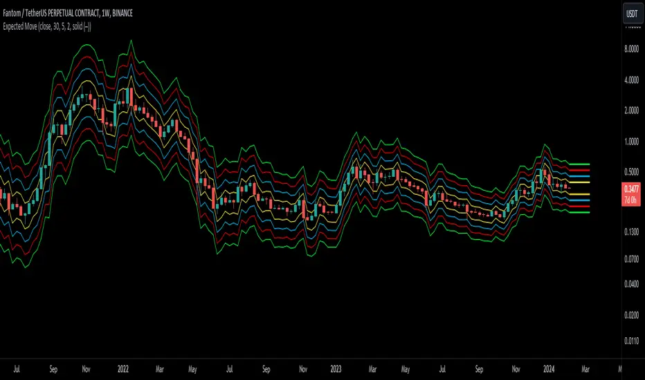
Expected Move BandsExpected Moves
The Expected Move of a security shows the amount that a stock is expected to rise or fall from its current market price based on its level of volatility or implied volatility. The expected move of a stock is usually measured with standard deviations.
An Expected Move Range of 1 SD shows that price will be near the 1 SD range 68% of the time given enough samples.
Expected Move Bands
This indicator gets the Expected Move for 1-4 Standard Deviation Ranges using Historical Volatility. Then it displays it on price as bands.
The Expected Move indicator also allows you to see MTF Expected Moves if you want to.
This indicator calculates the expected price movements by analyzing the historical volatility of an asset. Volatility is the measure of fluctuation.
This script uses log returns for the historical volatility calculation which can be modelled as a normal distribution most of the time meaning it is symmetrical and stationary unlike other scripts that use bands to find "reversals". They are fundamentally incorrect.
What these ranges tell you is basically the odds of the price movement being between these levels.
If you take enough samples, 95.5% of the them will be near the 2nd Standard Deviation. And so on. (The 3rd Standard deviation is 99.7%)
For higher timeframes you might need a smaller sample size.
Features
MTF Option
Parameter customization
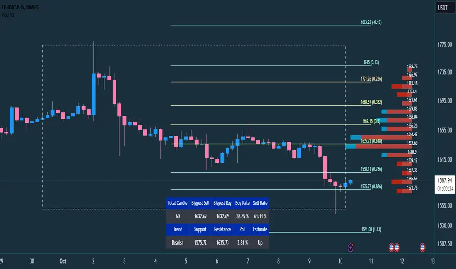
VIPER DOPING - A Volume Profile to estimate trend probabilityDESCRIPTION :
VIPER DOPING uses volume analysis to help trader to understand trading keys below:
Support and Resistance
Profit and Loss
Estimate candle direction
Trend
Biggest Buy and Sell on level prices
HOW TO USE:
The volume bar will have buy and sell colors, by default the buy color is blue and the sell is red. The size of bar is important matter, the biggest bar size means that price level has strong volume or transaction and the smallest bar size indicates the lowest transaction or volume. How to read it?
The bar above the candle is the resistance
The bar below the candle is the support
If you want long the market, find the biggest or bigger support, which is below the candle
If you want short the market, find the biggest or bigger resistance which is above the candle
Trading style and the maximum range (total candle), default is 60. This setup to analyze volumes in specific candle range. Please check the following recommendation based on trading style:
Scalping: 30 - 60 candles, recommendation timeframe: 5m - 1h
Day Trading: 50 - 120 candles, recommendation timeframe: 30m - 4h
Swing Trading: 100- 240 candles, recommendation timeframe: 1h- 3D
The white box is to visualize trading area by total candle. Every line has the meaning:
The left line is the start candle
The right line is the end candle
The top line is the highest price of volume profile
The bottom line is the lowest price of volume profile
The fibonacci line will help you to confirm and compare of supports and resistances with the volume profile lines.
The TABLE CELLS
it contains information to help trader to understand the recent situation of market and to take strategy of trading:
Total Candle : the maximum candles are used to analyze the volume from previous active candle
Biggest Sell : the horizontal price area which has the largest of sell volume of the last total candle
Biggest Buy : the horizontal price area which has the largest of buy volume of the last total candle
Buy Rate : the ratio of buy and sell volume of the last total candle
Support: the closest price to be the support from the active candle, auto changed if support to be invalid
Resistance : the closest price to be the resistance from the active candle, auto changed if support to be invalid
PnL : the percentage profit if you trade using the support and resistance prices and it can be used for Risk Management. Wisely the risk is 50% of the profit, example if the profit 1% the your risk should be 0.5% from entry.
Estimate : to analize the next direction of candle or target, it will be changed automatically by volume condition.
CONFIGURATION:
Table Position : You can change the table position to top or bottom, to left, right or center
Calculation : You can include the active candle in volume calculation or you can choose the behind active candle. If you use active candle, there could be possible repainting.
The volume profile configuration is about appearance configuration, to setup the thickness, colors, position.
The fibonacci configuration is about appearance configuration, to setup the thickness, extend lines, label styles.
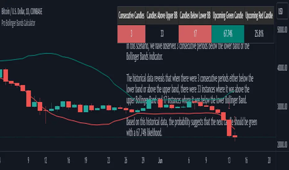
Pro Bollinger Bands CalculatorThe "Pro Bollinger Bands Calculator" indicator joins our suite of custom trading tools, which includes the "Pro Supertrend Calculator", the "Pro RSI Calculator" and the "Pro Momentum Calculator."
Expanding on this series, the "Pro Bollinger Bands Calculator" is tailored to offer traders deeper insights into market dynamics by harnessing the power of the Bollinger Bands indicator.
Its core mission remains unchanged: to scrutinize historical price data and provide informed predictions about future price movements, with a specific focus on detecting potential bullish (green) or bearish (red) candlestick patterns.
1. Bollinger Bands Calculation:
The indicator kicks off by computing the Bollinger Bands, a well-known volatility indicator. It calculates two pivotal Bollinger Bands parameters:
- Bollinger Bands Length: This parameter sets the lookback period for Bollinger Bands calculations.
- Bollinger Bands Deviation: It determines the deviation multiplier for the upper and lower bands, typically set at 2.0.
2. Visualizing Bollinger Bands:
The Bollinger Bands derived from the calculations are skillfully plotted on the price chart:
- Red Line: Represents the upper Bollinger Band during bearish trends, suggesting potential price declines.
- Teal Line: Represents the lower Bollinger Band in bullish market conditions, signaling the possibility of price increases.
3.Analyzing Consecutive Candlesticks:
The indicator's core functionality revolves around tracking consecutive candlestick patterns based on their relationship with the Bollinger Bands lines. To be considered for analysis, a candlestick must consistently close either above (green candles) or below (red candles) the Bollinger Bands lines for multiple consecutive periods.
4. Labeling and Enumeration:
To convey the count of consecutive candles displaying consistent trend behavior, the indicator meticulously assigns labels to the price chart. The position of these labels varies depending on the direction of the trend, appearing either below (for bullish patterns) or above (for bearish patterns) the candlesticks. The label colors match the candle colors: green labels for bullish candles and red labels for bearish ones.
5. Tabular Data Presentation:
The indicator complements its graphical analysis with a customizable table that prominently displays comprehensive statistical insights. Key data points within the table encompass:
- Consecutive Candles: The count of consecutive candles displaying consistent trend characteristics.
- Candles Above Upper BB: The number of candles closing above the upper Bollinger Band during the consecutive period.
- Candles Below Lower BB: The number of candles closing below the lower Bollinger Band during the consecutive period.
- Upcoming Green Candle: An estimated probability of the next candlestick being bullish, derived from historical data.
- Upcoming Red Candle: An estimated probability of the next candlestick being bearish, also based on historical data.
6. Custom Configuration:
To cater to diverse trading strategies and preferences, the indicator offers extensive customization options. Traders can fine-tune parameters such as Bollinger Bands length, upper and lower band deviations, label and table placement, and table size to align with their unique trading approaches.
Candles In Row (Expo)█ Overview
The Candles In Row (Expo) indicator is a powerful tool designed to track and visualize sequences of consecutive candlesticks in a price chart. Whether you're looking to gauge momentum or determine the prevailing trend, this indicator offers versatile functionality tailored to the needs of active traders. The Candles In Row indicator can be an integral part of a multi-timeframe trading strategy, allowing traders to understand market momentum, and set trading bias. By recognizing the patterns and likelihood of future price movements, traders can make more informed decisions and align their trades with the overall market direction.
█ How to use
The indicator enhances traders' understanding of the consecutive candle patterns, helping them to uncover trends and momentum. Consecutive candles in the same direction may indicate a strong trend. The Candles In Row indicator can be an essential tool for traders employing a multiple timeframes strategy.
Analyzing a Higher Timeframe:
Understanding Momentum: By analyzing consecutive green or red candles in a higher timeframe, traders can identify the prevailing momentum in the market. A series of green candles would suggest an upward trend, while a series of red candles would indicate a downward trend.
Predicting Next Candle: The indicator's predictive feature calculates the likelihood of the next candle being green or red based on historical patterns. This probability helps traders gauge the potential continuation of the trend.
Setting the Trading Bias: If the likelihood of the next candle being green is high, the trader may decide to focus on long (buy) opportunities. Conversely, if the likelihood of the next candle being red is high, the trader may look for short (sell) opportunities.
In this example, we are using the Heikin Ashi candles.
Moving to a Lower Timeframe:
Finding Entry Points: Once the trading bias is set based on the higher timeframe analysis, traders can switch to a lower timeframe to look for entry points in the direction of the bias. For example, if the higher timeframe suggests a high likelihood of a green candle, traders may look for buy opportunities in the lower timeframe.
Combining Timeframes for a Comprehensive Strategy:
Confirmation and Alignment: By analyzing the higher timeframe and confirming the direction in the lower timeframe, traders can ensure that they are trading in alignment with the broader trend.
Avoiding False Signals: By using a higher timeframe to set the trading bias and a lower timeframe to find entries, traders can avoid false signals and whipsaws that might be present in a single timeframe analysis.
█ Settings
Price Input Selection: Choose between regular open and close prices or Heikin Ashi candles as the basis for calculation.
Data Window Control: Decide between displaying the full data window or only the active data. You can also enable a counter that keeps track of the number of candles.
Alert Configuration: Set the desired number and color of consecutive candles that must occur in a row to trigger an alert.
Table Display Customization: Customize the location and size of the display table according to your preferences.
-----------------
Disclaimer
The information contained in my Scripts/Indicators/Ideas/Algos/Systems does not constitute financial advice or a solicitation to buy or sell any securities of any type. I will not accept liability for any loss or damage, including without limitation any loss of profit, which may arise directly or indirectly from the use of or reliance on such information.
All investments involve risk, and the past performance of a security, industry, sector, market, financial product, trading strategy, backtest, or individual's trading does not guarantee future results or returns. Investors are fully responsible for any investment decisions they make. Such decisions should be based solely on an evaluation of their financial circumstances, investment objectives, risk tolerance, and liquidity needs.
My Scripts/Indicators/Ideas/Algos/Systems are only for educational purposes!

Normal Distribution CurveThis Normal Distribution Curve is designed to overlay a simple normal distribution curve on top of any TradingView indicator. This curve represents a probability distribution for a given dataset and can be used to gain insights into the likelihood of various data levels occurring within a specified range, providing traders and investors with a clear visualization of the distribution of values within a specific dataset. With the only inputs being the variable source and plot colour, I think this is by far the simplest and most intuitive iteration of any statistical analysis based indicator I've seen here!
Traders can quickly assess how data clusters around the mean in a bell curve and easily see the percentile frequency of the data; or perhaps with both and upper and lower peaks identify likely periods of upcoming volatility or mean reversion. Facilitating the identification of outliers was my main purpose when creating this tool, I believed fixed values for upper/lower bounds within most indicators are too static and do not dynamically fit the vastly different movements of all assets and timeframes - and being able to easily understand the spread of information simplifies the process of identifying key regions to take action.
The curve's tails, representing the extreme percentiles, can help identify outliers and potential areas of price reversal or trend acceleration. For example using the RSI which typically has static levels of 70 and 30, which will be breached considerably more on a less liquid or more volatile asset and therefore reduce the actionable effectiveness of the indicator, likewise for an asset with little to no directional volatility failing to ever reach this overbought/oversold areas. It makes considerably more sense to look for the top/bottom 5% or 10% levels of outlying data which are automatically calculated with this indicator, and may be a noticeable distance from the 70 and 30 values, as regions to be observing for your investing.
This normal distribution curve employs percentile linear interpolation to calculate the distribution. This interpolation technique considers the nearest data points and calculates the price values between them. This process ensures a smooth curve that accurately represents the probability distribution, even for percentiles not directly present in the original dataset; and applicable to any asset regardless of timeframe. The lookback period is set to a value of 5000 which should ensure ample data is taken into calculation and consideration without surpassing any TradingView constraints and limitations, for datasets smaller than this the indicator will adjust the length to just include all data. The labels providing the percentile and average levels can also be removed in the style tab if preferred.
Additionally, as an unplanned benefit is its applicability to the underlying price data as well as any derived indicators. Turning it into something comparable to a volume profile indicator but based on the time an assets price was within a specific range as opposed to the volume. This can therefore be used as a tool for identifying potential support and resistance zones, as well as areas that mark market inefficiencies as price rapidly accelerated through. This may then give a cleaner outlook as it eliminates the potential drawbacks of volume based profiles that maybe don't collate all exchange data or are misrepresented due to large unforeseen increases/decreases underlying capital inflows/outflows.
Thanks to @ALifeToMake, @Bjorgum, vgladkov on stackoverflow (and possibly some chatGPT!) for all the assistance in bringing this indicator to life. I really hope every user can find some use from this and help bring a unique and data driven perspective to their decision making. And make sure to please share any original implementaions of this tool too! If you've managed to apply this to the average price change once you've entered your position to better manage your trade management, or maybe overlaying on an implied volatility indicator to identify potential options arbitrage opportunities; let me know! And of course if anyone has any issues, questions, queries or requests please feel free to reach out! Thanks and enjoy.

Probability Box Rule of Thirds [PPI]█ Probability Box Rule of Thirds
The Probability Box Rule of Thirds , is a visual indicator that helps traders identify possible overbought and oversold conditions. It does this by dividing the price range – highest high minus the lowest low of a given lookback period or date range – into thirds. Each third has distinct probability characteristics and when combined represent a probability box.
We have spent years refining the probability box concept, and have previously published a How To on Trading View – "How to Trade Probability Ranges – The Critical Rule of 1/3" which can be found here:
To quickly summarize the How To – when using the Rule of Thirds , you are using a combination of statistics, probabilities of success, and prior price action to determine when to enter a trade. The visual range division helps remove subjectivity and clearly shows when the trading odds are stacked in your favor. By identifying and taking higher probability trades, you have a higher chance of success as trading is all about probability and risk management.
Implementing the Rule of Thirds starts with finding an instrument that is consolidating and identifying the nearest important support and resistance levels based on your targeted trading timeframe or lookback period.
The range between the support and resistance levels is divided into thirds to form three zones within the consolidation range.
When going LONG , you want to BUY in the bottom third of the range. Once you buy, your objective is to hold during the middle third and sell when the price enters the top third.
When you buy in the lower third, there's a 66.6% probability of success. If you buy in the middle third, you only have a 50% / 50% chance of success. Going long in the top third of the range gives you a 33.3% chance of success as you are already close to the identified resistance level.
When going SHORT , the sequence and odds are reversed. You want to SELL in the top third of the range, hold the middle third and exit in the bottom third of the range. This gives you a 66.6% chance of success when entering in the top third, a 50% / 50% chance when entering in the middle third, and a 33.3% chance in the bottom third given you are already close to the identified support level.
When the price lies in the middle third, the even 50% / 50% odds provide no probability edge and a trader is better off waiting until the price reaches the upper or lower thirds of the price range.
The Rule of Thirds allows us to quickly visually evaluate trades based on probabilities, selectively enter trades that have the highest odds of success, and avoid likely losing trades. The Rule of Thirds gives you confidence to hold trades based on prior trading ranges and provides clear levels where the prices are likely to either reverse or start trending.
The Probability Box Rule of Thirds automatically implements the first two steps of the Rule of Thirds by using the highest high and lowest low of a given lookback period to identify the support and resistance levels, and automatically divides the range into thirds. The rest of the Rule of Thirds rules remain the same.
Just having the price within the bottom thirds or top thirds, however, does not mean the price will immediately reverse. The GE chart below is an example of a stock that remained 'stuck' in the upper thirds of the price range for an extended amount of time:
And the CVS chart below is an example where the price is 'stuck' in the lower thirds of the price range:
While the price is in the upper or lower thirds, it is very important that the trader should use other indicators to identify when a significant trend reversal occurs. Once a trend reversal event happens, the trader either enters a trade AND/OR exits a trade if already in one.
When the price exceeds the bounds of the probability box, there are three possible outcomes – a strong continuation trend, the price consolidates around the probability box edge, or a trend reversal. Your favorite indicators will help determine which event is happening.
The CVS chart above is a good example of the probability box being exceeded with the last bar. The price exceeding the price range is temporary event as the price range will expand to encompass the revised price range on the next trading day.
█ Indicator Features
Each supported timeframe – Monthly, Weekly, and Daily – allows the selection of an appropriate lookback period for your trading style. The defaults are a good starting point for swing trading and long-term investing. You many need to experiment to find the optimal lookback period for your trading style.
Even if you only day trade, the Probability Box Rule of Thirds with the appropriate lookback periods can help you visualize the bigger picture of where the instrument is heading.
When viewing the charts, you can find the currently selected lookback period above the upper edge of the price range.
The indicator will display a dotted yellow line at 50% of the price range and show the line's value when requested.
The visibility of the actual thirds and border price values are controlled by the " Show Probability Box Values " checkbox. You may need to expand the chart's right margin to see the values.
The " Show Internal Labels " checkbox controls the display of the internal ⅓ Division labels and the percentage odds, along with the 50% label. This option by default is set to off.
The " Show Error Messages " checkbox controls the display of error messages and by default is turned on. Turn off to prevent error messages from being shown on intraday timeframes. Save as indicator default to prevent having to turn off this setting each time added to chart.
The color and transparency controls allow the user to modify the colors used for each third. The default settings are optimized for use with a DARK background.
█ Implementation Notes
IMPORTANT - the Probability Box Rule of Thirds is set up to only handle Monthly, Weekly and Daily charts. This is intentional as the indicator is designed to be used for safer multiple day and longer swing trades. When viewed on intraday charts, the indicator will be hidden.
The Probability Box Rule of Thirds uses a rolling window of the equivalent number of bars for the lookback period rather than relying on the bar starting and ending dates. This allows the use of a standard number of days in the selected lookback window across various instruments and ensures fast, efficient calculations.
The lookback periods are adjusted when non-standard timeframe multipliers are used – e.g., a 12M chart timeframe and a 3-year lookback period will result in a 3 bar lookback. Fractional bars in this calculation are rounded up and any incompatible lookback period and chart timeframe combination will generate a runtime error.
In summary, the Probability Box Rule of Thirds automates and visually identifies overbought and oversold areas, which combined with the Rule of Thirds probability risk profiles, increases your odds of success through better trade selections and higher confidence in your trades.
█ Disclaimer
There is substantial risk in trading. Losses incurred in trading can be significant. Only trade with money you can afford to lose. We make no claims whatsoever regarding the impact of past or future performance on your trading results.
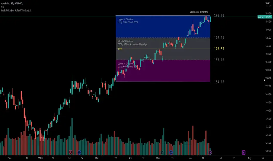
Probability Trend IndicatorUnderstanding the Indicator:
The indicator calculates the probabilities of upward and downward trends based on the percentage change in price over a specified lookback period.
It displays these probabilities in a table and plots a histogram to represent the difference between the probabilities.
The colors of the histogram bars indicate the trend direction and whether the trend is increasing or decreasing.
Setting the Lookback Period:
The indicator allows you to specify the lookback period, which determines the number of bars to consider for calculating the probabilities.
By default, the lookback period is set to 50 bars. However, you can adjust it based on your trading preferences and the timeframe you're analyzing.
Analyzing the Probabilities:
The indicator calculates the probabilities of upward and downward trends and displays them in a table on the chart.
The probabilities are presented as percentages, representing the likelihood of each type of trend occurring.
You can use these probabilities to gain insights into the potential market direction and assess the strength of the prevailing trend.
Interpreting the Histogram:
The histogram is plotted based on the difference between the probabilities of upward and downward trends, known as the oscillator value.
The histogram bars are colored to provide visual cues about the trend direction and whether the trend is gaining or losing strength.
Green bars indicate upward trends, and red bars indicate downward trends.
Lighter shades of green or red suggest increasing trends, while darker shades suggest decreasing trends.
Making Trading Decisions:
The indicator serves as a tool for assessing the probabilities of trends and can be used alongside other technical analysis methods.
You can consider the probabilities, the histogram pattern, and the overall market context to make informed trading decisions.
It's important to remember that no indicator or tool can guarantee future market movements, so prudent risk management and additional analysis are essential.

Trend Reversal Probability CalculatorThe "Trend Reversal Probability Calculator" is a TradingView indicator that calculates the probability of a trend reversal based on the crossover of multiple moving averages and the rate of change (ROC) of their slopes. This indicator is designed to help traders identify potential trend reversals by providing signals when the short-term moving averages start to slope in the opposite direction of the long-term moving average.
To use the indicator, simply add it to your TradingView chart and adjust the input parameters according to your preferences. The input parameters include the length of the moving averages, the ROC length (trend sensitivity), and the reversal sensitivity (signal percentage).
The indicator calculates the ROC of the moving averages and determines if the short-term moving averages are sloping in the opposite direction of the long-term moving average. The number of short-term moving averages that meet this condition is then counted, and the probability of a trend reversal is calculated based on the percentage of short-term moving averages that meet this condition.
When the probability of a trend reversal is high, a bullish or bearish signal is generated, depending on the direction of the reversal. The bullish signal is generated when the short-term moving averages start to slope upward, and the bearish signal is generated when the short-term moving averages start to slope downward.
Traders can use the "Trend Reversal Probability Calculator" to identify potential trend reversals and adjust their trading strategies accordingly. It is important to note that this indicator is not a guarantee of a trend reversal and should be used in conjunction with other technical analysis tools to make informed trading decisions.

Bayesian predictive leading indicator--------- ENGLISH ---------
This is a predictive indicator ( leading indicator ) that uses Bayes' formula to calculate the conditional probability of price increases given the angular coefficient. The indicator calculates the angular coefficient and its regression and uses it to predict prices.
Bayes' theorem is a fundamental result of probability theory and is used to calculate the probability of a cause causing the verified event. In other words, for our indicator, Bayes' theorem is used to calculate the conditional probability of one event (price event in this case) with respect to another event by calculating the probabilities of the two events (past price) and the conditional probability of the second event (future price) with respect to the first event.
The red line represents the angular coefficient. The blue line represents the normalized expected price. Finally, the yellow line represents the conditional probability that the price will increase or decrease.
How to use it. In addition to the convenient histogram, which follows the angular coefficient, another practical operational application might be to go long when the blue line is above the red and yellow lines. Conversely short when the blue is below the red and yellow.
When the yellow line passes above all others, a reversal in the long direction is imminent and vice versa.
The extent of the reversal depends on how far the yellow line will be away in price from the other 2 lines.
This indicator is in its embryonic state and updates will follow to make it more graphically readable, add alerts, etc.
Stay tuned! Leave a boost and comment or write to me if you wish.
--------- ITALIANO ---------
Questo è un indicatore predittivo ( leading indicator ) che utilizza la formula di Bayes per calcolare la probabilità condizionata che il prezzo aumenti dato il coefficiente angolare. L’indicatore calcola il coefficiente angolare e la sua regressione e lo utilizza per prevedere i prezzi.
Il teorema di Bayes è un risultato fondamentale della teoria della probabilità e viene impiegato per calcolare la probabilità di una causa che ha provocato l’evento verificato. In altre parole, per il nostro indicatore, il teorema di Bayes serve per calcolare la probabilità condizionata di un evento (di prezzo in questo caso) rispetto a un altro evento, calcolando le probabilità dei due eventi (prezzo passato) e la probabilità condizionata del secondo evento (prezzo futuro) rispetto al primo.
La linea rossa rappresenta il coefficiente angolare. La linea blu rappresenta il prezzo previsto normalizzato. Infine la linea gialla rappresenta la probabilità condizionata che il prezzo aumenti o diminuisca.
Come si usa? Oltre al comodo istogramma, che segue il coefficiente angolare, un'altra applicazione operativa pratica potrebbe essere di andare long quando la linea blu è sopra la linea rossa e gialla. Viceversa short quando la blu è sotto la rossa e la gialla.
Quando la linea gialla passa sopra tutte le altre è imminente un'inversione in direzione long e viceversa.
L'entità dell'inversione dipende da quanto la linea gialla sarà distante di prezzo dalle altre 2 linee.
Questo indicatore è al suo stato embrionale e seguiranno aggiornamenti per renderlo graficamente più leggibile, aggiungere alert, ecc.
Stay tuned! Lascia un boost e commenta o scrivimi se desideri.
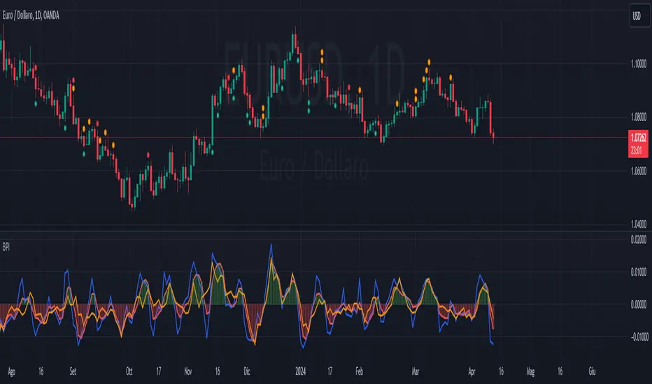
VS Score [SpiritualHealer117]An experimental indicator that uses historical prices and readings of technical indicators to give the probability that stock and crypto prices will be in a certain range on the next close. This indicator may be helpful for options traders or for traders who want to see the probability of a move.
It classifies returns into five categories:
Extreme Rise - Over 2 standard deviations above normal returns
Rise - Between 0.5 standard deviations and 2 standard deviations above normal returns
Flat - Falling in the range of +/- 0.5 standard deviations of normal returns
Fall - Between 0.5 standard deviations and 2 standard deviations below normal returns
Extreme Fall - Over 2 standard deviations below normal returns
It is an adaptive probability model, which trains on the previous 1000 data points, and is calculated by creating probability vectors for the current reading of the PPO, MA, volume histogram, and previous return, and combining them into one probability vector.

Quantitative Price Forecasting - The Quant ScienceThis script is a quantitative price forecasting indicator that forecasts price changes for a given asset.
The model aims to forecast future prices by analyzing past data within a selected time period. Mathematical probability is used to calculate whether starting from time X can lead to reaching prices Y1 and Y2. In this context, X represents the current selected time period, Y1 represents the selected percentage decrease, and Y2 represents the selected percentage increase. The probabilities are estimated using the simple average.
The simple average is displayed on the chart, showing in red the periods where the price is below the average and in green the periods where the price is above the average.
This powerful tool not only provides forecasts of future prices but also calculates the distribution of variations around the average. It then takes this information and creates an estimate of the average price variation around the simple average.
Using a mean-reverting logic, buying and selling opportunities are highlighted.
We recommend turning off the display of bars on your chart for a better experience when using this indicator.
Unlock the full potential of your trading strategy with our powerful indicator. By analyzing past price data, it provides accurate forecasts and calculates the probability of reaching specific price targets. Its mean-reverting logic highlights buying and selling opportunities, while the simple moving average displayed on the chart shows periods where the price is above or below the average. Additionally, it estimates the average variation of price around the simple average, giving you valuable insights into price movements. Don't miss out on this valuable tool that can take your trading to the next level