Smoothed Heikin Ashi Trend on Chart - TraderHalai BACKTESTSmoothed Heikin Ashi Trend on chart - Backtest
This is a backtest of the Smoothed Heikin Ashi Trend indicator, which computes the reverse candle close price required to flip a Heikin Ashi trend from red to green and vice versa. The original indicator can be found in the scripts section of my profile.
This particular back test uses this indicator with a Trend following paradigm with a percentage-based stop loss.
Note, that backtesting performance is not always indicative of future performance, but it does provide some basis for further development and walk-forward / live testing.
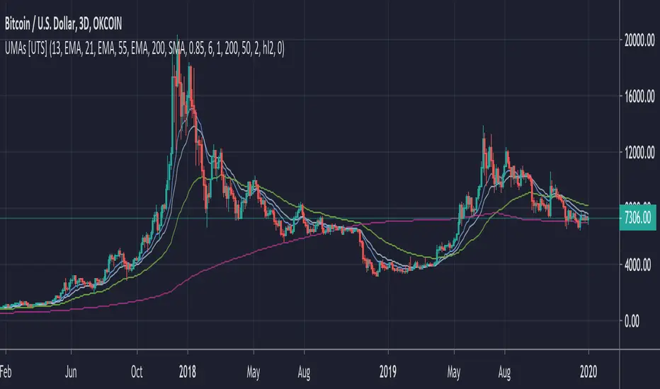
Testing was performed on Bitcoin , as this is a primary target market for me to use this kind of strategy.
Sample Backtesting results as of 10th June 2022:
Backtesting parameters:
Position size: 10% of equity
Long stop: 1% below entry
Short stop: 1% above entry
Repainting: Off
Smoothing: SMA
Period: 10
8 Hour:
Number of Trades: 1046
Gross Return: 249.27 %
CAGR Return: 14.04 %
Max Drawdown: 7.9 %
Win percentage: 28.01 %
Profit Factor (Expectancy): 2.019
Average Loss: 0.33 %
Average Win: 1.69 %
Average Time for Loss: 1 day
Average Time for Win: 5.33 days
1 Day:
Number of Trades: 429
Gross Return: 458.4 %
CAGR Return: 15.76 %
Max Drawdown: 6.37 %
Profit Factor (Expectancy): 2.804
Average Loss: 0.8 %
Average Win: 7.2 %
Average Time for Loss: 3 days
Average Time for Win: 16 days
5 Day:
Number of Trades: 69
Gross Return: 1614.9 %
CAGR Return: 26.7 %
Max Drawdown: 5.7 %
Profit Factor (Expectancy): 10.451
Average Loss: 3.64 %
Average Win: 81.17 %
Average Time for Loss: 15 days
Average Time for Win: 85 days
Analysis:
The strategy is typical amongst trend following strategies with a less regular win rate, but where profits are more significant than losses. Most of the losses are in sideways, low volatility markets. This strategy performs better on higher timeframes, where it shows a positive expectancy of the strategy.
The average win was positively impacted by Bitcoin’s earlier smaller market cap, as the percentage wins earlier were higher.
Overall the strategy shows potential for further development and may be suitable for walk-forward testing and out of sample analysis to be considered for a demo trading account.
Note in an actual trading setup, you may wish to use this with volatility filters, combined with support resistance zones for a better setup.
As always, this post/indicator/strategy is not financial advice, and please do your due diligence before trading this live.
Original indicator links:
On chart version -
Oscillator version -
Update - 27/06/2022
Unfortunately, It appears that the original script had been taken down due to auto-moderation because of concerns with no slippage / commission. I have since adjusted the backtest, and re-uploaded to include the following to address these concerns, and show that I am genuinely trying to give back to the community and not mislead anyone:
1) Include commission of 0.1% - to match Binance's maker fees prior to moving to a fee-less model.
2) Include slippage of 10 ticks (This is a realistic slippage figure from searching online for most crypto exchanges)
3) Adjust account balance to 10,000 - since most of us are not millionaires.
The rest of the backtesting parameters are comparable to previous results:
Backtesting parameters:
Initial capital: 10000 dollars
Position size: 10% of equity
Long stop: 2% below entry
Short stop: 2% above entry
Repainting: Off
Smoothing: SMA
Period: 10
Slippage: 10 ticks
Commission: 0.1%
This script still remains to shows viability / profitablity on higher term timeframes (with slightly higher drawdown), and I have included the backtest report below to document my findings:
8 Hour:
Number of Trades: 1082
Gross Return: 233.02%
CAGR Return: 14.04 %
Max Drawdown: 7.9 %
Win percentage: 25.6%
Profit Factor (Expectancy): 1.627
Average Loss: 0.46 %
Average Win: 2.18 %
Average Time for Loss: 1.33 day
Average Time for Win: 7.33 days
Once again, please do your own research and due dillegence before trading this live. This post is for education and information purposes only, and should not be taken as financial advice.
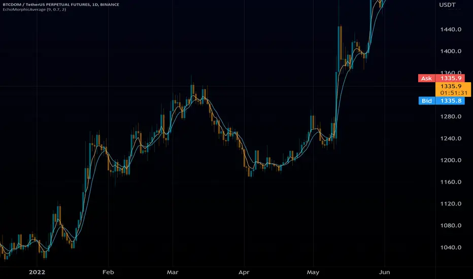
Smooth

EchoMorphicAverageLibrary "EchoMorphicAverage"
Original Self Referencing Moving Average which references
it's own output agsainst itself and the incoming source to dynamically
alter smoothness and length internally per calculation cycle.
@kaigouthro
Inputs are float length series.
Contact Me for More Dynamic Float Length Indicators.
wema(src, mod, len)
Waited Echo-Morphic Average
Parameters:
src : (float) input value
mod : (float) modifier(0-1) mix of current value
len : (float) length
Returns: output processed smoothed value
wemaStack(src, mod, len)
Stacked Multipass Waited Echo-Morphic Average
Parameters:
src : (float) input value
mod : (float) modifier(0-1) mix of current value
len : (float) length
Returns: output processed smoothed value
Heikin Ashi Volatility Percentile - TraderHalaiThe Heikin Ashi Volatility Percentile (HAVP) Oscillator was inspired by the legendary Bollinger Band Width Percentile indicator(known as BBWP), written by Caretaker, and made famous by Eric Krown, a famous influencer.
This script borrows aspects of the BBWP indicator which enables the HAVP oscillator to visually match the look and feel of BBWP and allows similar configuration functions (such as colouring function, smoothing MAs and alerts)
The fundamentals of this script are however different to BBWP. Instead of Bollinger band width, this script uses a reverse function of Heikin Ashi close (implemented in my Smoothed Heikin Ashi Trend
indicator, linked below).
The reverse Heikin Ashi close is smoothed using Ehler's SuperSmoother function, providing smooth oscillation and earlier signals of volatility tops and bottoms.
From an automated backtest that I have conducted on the BTCUSD index pair, I have observed comparable performance to BBWP across multiple timeframes when combining with stochastic direction to give a bias on overall direction. Using parameters I have tested, it performs better on mid-term timeframes such as 3h,4h and 6h. BBWP outperforms on 1h and 1d, with lower timeframes being comparable.
From the results, using HAVP over BBWP tends to result in reduced holding time and more frequent trades, which may or may not be desirable, although the behaviour can be adjusted using the parameters provided.
For instance, the smoother oscillation provided by HAVP provides a great predictability factor and earlier confirmation signals, which is something that Ehler emphasised in his trading style, and something which I agree with personally. I would encourage you to try out both HAVP and BBWP and see which fits your trading style.
Releasing this as open source allows for the betterment of the community and further development, criticism and discussion.
Thanks and enjoy! :)

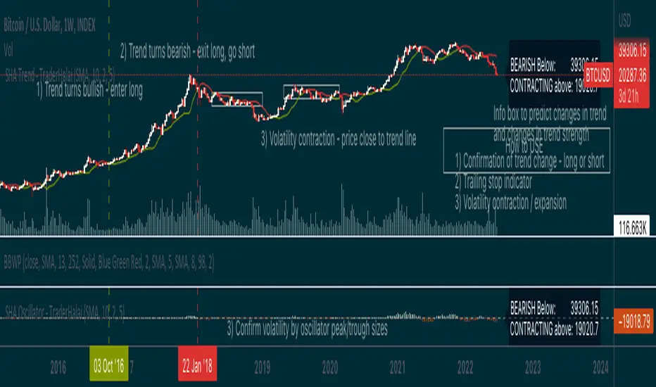
Smoothed Heikin Ashi Trend on Chart - TraderHalaiThis indicator is a predictive tool using Heikinashi to calculate shifts in trade direction.
It works by reverse-engineering the regular candle stick closing price required, to flip the Heiken Ashi candle from Red to Green and vice-versa.
Below, is an earlier indicator that I released and created. This plots this price as an oscillator, which allows traders to get a predictive indicator of a trend change.
This indicator extends upon this functionality by adding a smoothing function to the reverse-engineered regular candle stick closing price, to reduce the choppiness of signals. It also plots the indicator on the chart to allow for easier visual confirmation.
How to use
1) As a directional bias - Bullish or bearish
2) Volatility expansion/contraction - further distance from line means volatility expansion - am planning to release an oscillator version also
3) Trailing stop loss - once you are in a trade
Other Features
Select a moving average period and smoothing calculation method (e.g. SMA / EMA)
Non-repaint mode for backtesting and use/integration with higher timeframes
Final note - Open Source
I am releasing this as open-source for the benefit of the community and to allow further development, scrutiny and criticism. Please feel free to use this indicator as you see fit. If you do use this indicator to create another script, feel free to drop me a note, as I would be highly interested in your idea.
Thanks, and Enjoy!
High-Low IndexHello All,
High-Low Index is a breadth indicator based on Record High Percent (RHP). RHP is based on new 52-week highs and new 52-week lows. RHP => 100 * (new highs) / (new highs + new lows). High-Low Index is a 10-day Simple Moving Average of the RHP, which makes it a smoothed version of RHP. You can find many articles about High-Low Index on the net.
High-Low Index above 50 indicates that there are more new highs than new lows, and considered as Bullish.
High-Low Index below 50 indicates that there are more new lows than new highs, and considered as Bearish.
High-Low Index = 0 indicates there is no new highs (0% new highs).
High-Low Index = 100 indicates that there is at least 1 new high and no new lows.
and High-Low Index = 50 indicates that new highs and new lows is equal.
by default 40 cryptos are used in the script and shows High-Low Index for these cryptos. but you can change them as you wish. for example you can set all of them as stocks and see High-Low Index for these stocks.
You can set " Time frame " and the " Length " using the options. For example; if you set " Time frame " = 1 Week and the " Length " = 52 then it finds High-Low Index for 52weeks .
or another example; if you set " Time frame " = 1 Day and the " Length " = 22 the High-Low Indexn it finds High-Low Index for 22days.
You can enable/disable Record High Percent or Simple Moving Average of High-Low Index. Some traders use High-Low Index with its SMA, for example; High-Low Index generates a buy signal when it crosses above its moving average, and a sell signal when it crosses below its moving average.
Optionally you can see the securities in a table on the left bottom, you can change table size by usşng the options.
In the Table, for each security/cell;
=> if background is green then it has New High
=> if background is red then it has New Low
=> if background is gray then no New High, no New Low
=> if background is back then Data is not available for the security
As you can see in the screenshot below, the securities were changed and stocks are used instead of cryptos, so it calculates & shows High-Low Index for these stocks.
you can also find explanation in this screenshot:
Enjoy!

AnalysisInterpolationLoessLibrary "AnalysisInterpolationLoess"
LOESS, local weighted Smoothing function.
loess(sample_x, sample_y, point_span) LOESS, local weighted Smoothing function.
Parameters:
sample_x : int array, x values.
sample_y : float array, y values.
point_span : int, local point interval span.
aloess(sample_x, sample_y, point_span) aLOESS, adaptive local weighted Smoothing function.
Parameters:
sample_x : int array, x values.
sample_y : float array, y values.
point_span : int, local point interval span.

%-[Guz] Vortex Indicator Custom// Custom Vortex Strategy (backtester)
// Custom version of the Vortex indicators that adds many features:
// -Triggers trades after a threshold is reached instead of the normal vortex lines cross (once the difference between the 2 lines is important enough)
// -Smooths the Vortex lines with an EMA
// -Adds Take Profit and Stop Loss selection
// -Adds the possibility to go Long only, Short only or both of them
// ! notice that it uses 10% position size and 0.04% trade fee, found on some crypto exchanges futures contracts
// Allows testing leverage with position size modification (values above 100% position size, to be done with caution)
// Not an investment advice

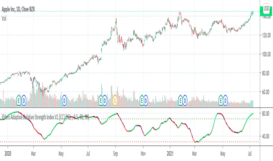
Ehlers Adaptive Relative Strength Index V1 [CC]The Adaptive Relative Strength Index was created by John Ehlers and this is his first version. I will of course publish his updated version at a later date along with publishing the final script from Jim Sloman's Ocean Theory book. I have changed his script to include extra smoothing to provide clear buy and sell signals. This is a version of a RSI that is very adaptive to changes by finding the length of the current cycle and using that to calculate the rsi and I use this same basic process to provide extra smoothing. A great strategy of course is to buy right after the indicator goes from below the oversold level to right above it and stay in until the indicator turns red or when it reaches the overbought level. I have included strong buy and sell signals in addition to normal ones and the darker colors mean strong signals and lighter colors are normal signals.
Let me know what other indicators you would like to see me publish!
Heikin Ashi Candle OverlayHello Friend,
This is a very simple script for fun to demonstrate the new ability to change the colors of attributes pertaining to the plotbar() and plotcandle() functions using series inputs.
For Heiken Ashi lovers, this script does several things. It gives you both bars and hollow candles with Heikin Ashi values - something TV does not currently support.
It also gives you the ability to see your favorite HA candles while on the main series plot. When viewing indicators in the "Heikin Ashi" candle setting on TradingView, the input values are "smoothed' with HA values. This skews the way your indicators behave as the OLHC are calculated averages. Only the regular candle settings will give your indicators "real close" etc.
By 'Muting' the main series bars by toggling the 👁 symbol next to your ticker id, it makes the normal candles invisible. You then overlay this script, which allows you to see the HA Candle of your choice, while not affecting the way your indicators behave.
You now have the best of 2 worlds. Smoothed behavior of price action to help visualize trends, and accurate indicator values derived from actual OLHC data.
Plus, something about hollow HA candles is just kind of clean and soothing isn't it?
Cheers,
Bjorgum
Hollow Setting:
Bars
Or just plain old regular, but on the main chart

Ehlers Smoothed Adaptive Momentum [CC]The Smoothed Adaptive Momentum indicator was created by John Ehlers and this indicator gives a lot of useful information. When the indicator is above 0 then there is very strong upward momentum and when the indicator falls below 0 then there is very strong downward momentum. A very profitable way to use this particular indicator is buy long when the indicator is below 0 and it crosses over it's signal line and then sell of course when you get the first sell signal. I have included strong buy and sell signals in addition to normal ones so darker colors mean strong signals and lighter colors are normal signals. Buy when the line turns green and sell when it turns red.
Let me know if you have any other scripts you would like to see me publish!

RedK Slow_Smooth Average (RSS_WMA)RedK Slow Smooth Average (RSS_WMA) is based on simple, multi-WMA passes to generate a moving average that sacrifices low-lag and fast responsiveness for the sake of smoothness.
This smoothness enables an increased trader ability to visualize and track longer-term trends and removes the noise of smaller, relatively insignificant price fluctuations.
Notes:
=========
* RSS_WMA is deliberately built to be a "lazy line" - and it works in a different way to other common moving averages that attempt to achieve less lag and quicker responsiveness - the idea and the use scenario is to act as a "smooth base" when used against a faster moving average like the v_Wave of the Co_Ra Wave
* Note that the settings of this line is "Smoothness' and not "length" - the initial length used for the first WMA pass calculation is 1/3 of that smoothness value selected in the settings
* Increments in the combined smoothness value will be allocated first to 1st WMA pass, then 2nd WMA pass, then 3rd pass consecutively then back to 1st pass.
* because we utilize 3 WMA passes, a settings below 3 will have no effect on the line and it will just track the "source" price.
Suggested Use:
===============
- Use RSS_WMA when you're looking for a smooth moving average that can help you analyze you chart at a broader / macro level, visualize the broader price action patterns and filter out the noise from short-term moves. you can also use this line to help set your position exits since only major and persistent moves will cause this line, as lay as it is, to swing from one direction to the other.
How does RSS_WMA compare?
============================
here's a quick view of how the RSS_WMA compared to other commonly used Moving Averages, including my recently published CoRa_Wave
Code is commented - please feel free to use and customize further - please share a comment if you found this useful in your chart analysis or trading.

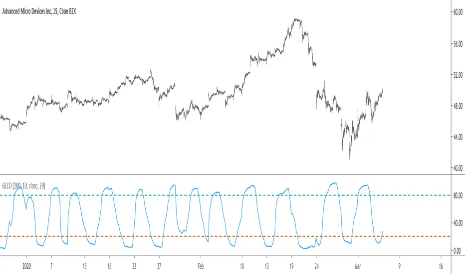
Trigonometric On Balance Volume (OBV) OscillatorLove volume analysis but it's hard for you to implement a simple strategy by it?
Use OBV.
Is OBV still not quite as it should be for you to get it in your trading system?
Use OBV Oscillator.
Does OBV Oscillator give you too many false signals and when you smooth it, it lags by a ton?
Then this indicator is the answer to your problem.
Introducing the Trigonometric OBV Oscillator.
The Trigonometric OBV Oscillator or "Trig OBV" for short, uses an old, but uniquely extremely reliable mathematical formula to smooth the OBV, while eliminating more than 95% of its false signals (noises) and keeping with the real direction of the trend without introducing any lags.
It is very responsive, predictive even to some degree, very reliable, and keeps you out of false trades (like false breakouts, sudden changes in the price, etc).
To go long: wait until the white line crosses up the purple line and continues in that direction.
To go short: wait until the white line crosses down the blue line and continues in that direction.
To exit, do the opposite.
Better to be used with a baseline filter such as Kaufman's moving average.
Use it and let me know what you think about it.

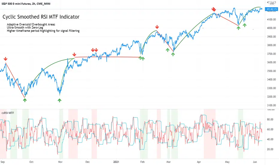
Cyclic Smoothed RSI MTFAdaptive cyclic smoothed Relative Strength Indicator (csRSI MTF)
The cyclic smoothed RSI MTF indicator is an enhancement of the RSI , adding zero-lag smoothing, adaptive oversold/overbought bands and period color highlighting from higher timeframe to filter signals.
Providing the following advanced features:
using the current dominant cycle length as input for the indicator to ensure more accurate change in trends,
additional smoothing without introducing lag and maintaining clear sharp turns for signal generation,
adaptive upper and lower bands to avoid whipsaw trades and adapt the indicator to trending/cyclic conditions,
using higher time-frame csRSI oversold/overbought conditions to automatically highlight time windows with green/red backgrounds on the indicator panel for signal filtering and/or alert rules,
can be used to trigger alerts on your key symbols to get informed when a red/green windows are reached.
The following common problems with standard indicators are solved by this indicator:
First, normal indicators introduce a lot of false signals due to their noisy signal line. Second, to compensate for the noise, one would normally try to add some smoothing. But this only results in adding more delay to the indicator, which makes it almost useless. Third, oscillators contain static threshold levels to define oversold/overbought conditions. However, the market is not static and changes between trending and cycling periods. In trending periods, these static oversold/overbought levels are useless ore will trigger too much whipsaw trades. Finally, indicators don't take their state from other timeframes into account to filter signals.
All four problems described above are solved by the developed adaptive cyclic RSI with embedded MTF period highlighting.
Examples
S&P500 EMini Futures - csRSI 2H chart / 1D filter example signals
S&P E-Mini Futures 2h chart with daily higher time-frame filtering period for the csRSI, showing the standard RSI in the lower panel for signal comparison, signals from the csRSI are marked on the price chart
Bitcoin BTC /USD - csRSI 2H chart / 1D filter example signals
Bitcoin BTC /USD 2h chart with daily higher time-frame filtering period for the csRSI, signals marked
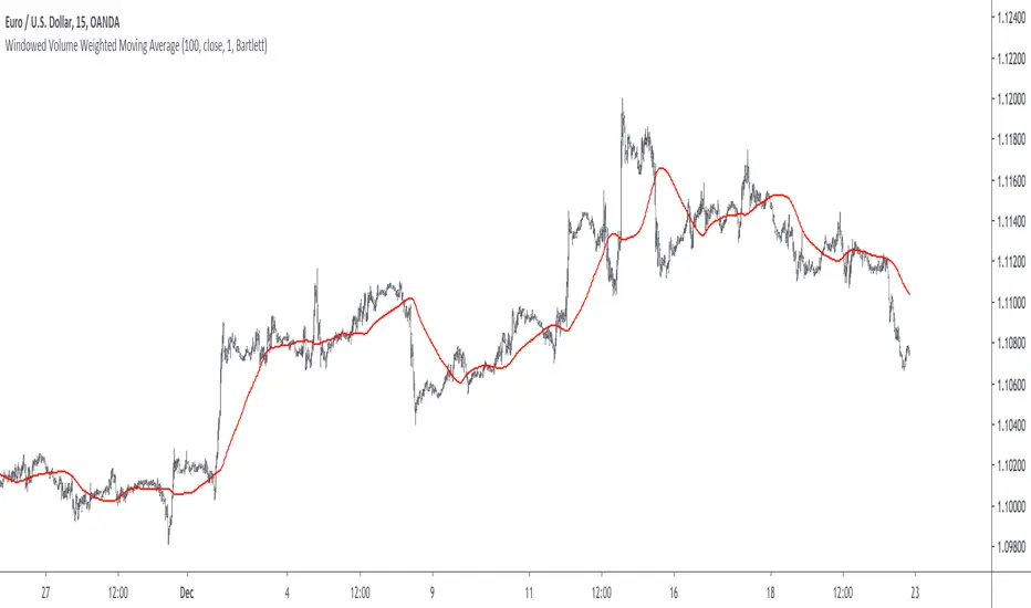
EUR/USD Forex - csRSI 20min chart / 2h filter example signals
EUR/USD 20min chart with 2H higher time-frame filtering period for the csRSI, signals marked
Info:
All three examples are setup with the basic standard settings and no additional parameter adjustments. The placed arrows on the price/indicator panel and the projection price areas have been added manually to visualize the signals for an discretionary trading approach. They are derived based on standard technical indicator oscillator readings (signal turn above/below bands). Due to the nature of the indicator (ultra-smooth, sharp curves, dynamic bands), these signals are easy to spot, and will help to avoid whipsaw trades in volatile conditions.
Settings & Parameter
The Inputs section allows you to select the time frame for the indicator signals. We recommend keeping the indicator time-frame according to your chart time frame ("Same as chart"). The cycle length allows to improve the signals by entering the dominant cycle length of the analyzed dataset. This parameter is optional if the current dominant cycle is not known. In that case, leave it at 20. The dominant cycle length can even improve the indicator signal generation. The examples above have not been optimized by using the dominant cycle length and just used the standard setting of 20.
The MTF CYCLE FILTER area is used to set the time-frame used as filter to plot the colored indicator background in red and green areas when the higher time-frame indicator is above (red) or below (green) the dynamic bands. These indicate the period of time with high probability to look for signals on the main indicator line.
The MTF Resolution parameter input is important for generating the highlighted red/green areas on the indicator panel. You must enter a higher time-frame than your indicator time-frame in order to get the reliable highlighting. We recommend the following combinations of trading time-frame and filter time-frame resolutions:
Chart Timeframe | MTF Indicator Highlighting Resolution
------------------------------------------------------------------------
20 min | 2 h
2 h | 1 d
You can enter the current dominant cycle length on the chosen higher time-frame resolution to even further optimize the indicator accuracy in the field "MTF CYCLE FILTER - Cycle Length".
The Style sections allows to active/de-active individual plots. The standard setting disables the higher time-frame csRSI indicator which is only used to indicate the colored areas. If required, you can also enable the MTF indicator and adaptive bands to be plotted in the same indicator panel. The values shown in the style section also indicate which values are available for individual alert generation.
Automatic Signals & Alerts
It is possible to create your own automatic signals with the csRSI MTF indicator using the TradingView alert function. Click on the three dots "More" beside the indicator name label and select "Add Alert on csRSI ..." from the context menu. For example, if you want to receive an alert when the high probability periods (red/green highlighted areas) have been reached for a symbol without manually watching the indicator panel, you can set up a custom alert. The csRSI indicator provides the raw values necessary to set up your alarm conditions. Set the "CSRSI MTF" as the value for the "Out of Channel" condition and select the "HigBand MTF" and "LowBand MTF" indicator values as the upper and lower limit parameters in the alarm's dialog box. Once you have set up this alarm, you will not need to monitor your charts manually. The TradingView alert will inform you as soon as an important time zone is reached. These are the situations when you would open the chart and watch for trigger signals on the indicator line. If you set up this alert as an email, you can even focus on other things and let the csRSI MTF highlighter condition alert you when you should pay attention to the trading chart.
Usage & Trade Signals
Classic rules apply as with every technical oscillator. In addition use this indicator to identify the following conditions:
Indicator turns above/below the adaptive upper and lower bands (expected trend reversals)
Indicator crosses below upper band / crossed above lower band (start of trend reversal)
Indicator crosses above upper band / crossed below lower band (trend continuation/confirmation)
Divergence between price / indicator indicate strong signal confidence
Hidden divergences between price/indicator indicate string signal confidence
After strong price movements, wait for the second signal confirmed by a divergence
Use the mentioned conditions in the highlighted red/green periods indicated by the MTF settings
Purpose & Disclaimer
This indicator is not designed for use as an automated trading strategy. This is an improved technical indicator using the dominant cycle to provide its advanced features. The basic applications of technical analysis for using oscillators apply. The script is intended for use in discretionary trading and can be used as a part of automated systems. Indicator signal failures will occur as you should expect with every technical indicator. If you are not sure if this indicator might help your trading style, please try and check our open source public version which will give you basic understanding upfront.
Basic open-source public version
This indicator is an advanced version of our public available open-source cyclic smoothed RSI indicator named "RSI cyclic smoothed v2". The advanced invite-only version provides fully automatic time frame highlighting by using a cyclically smoothed RSI from a higher time frame to indicate time frames with high probability signals. These high probability windows are highlighted when the indicator from the higher time frame is in dynamic overbought or oversold territory. You will find the basic open-source public version here below for your own review:
How to get access
Please check the "authors instructions" section for further details.
Skrip berbayar
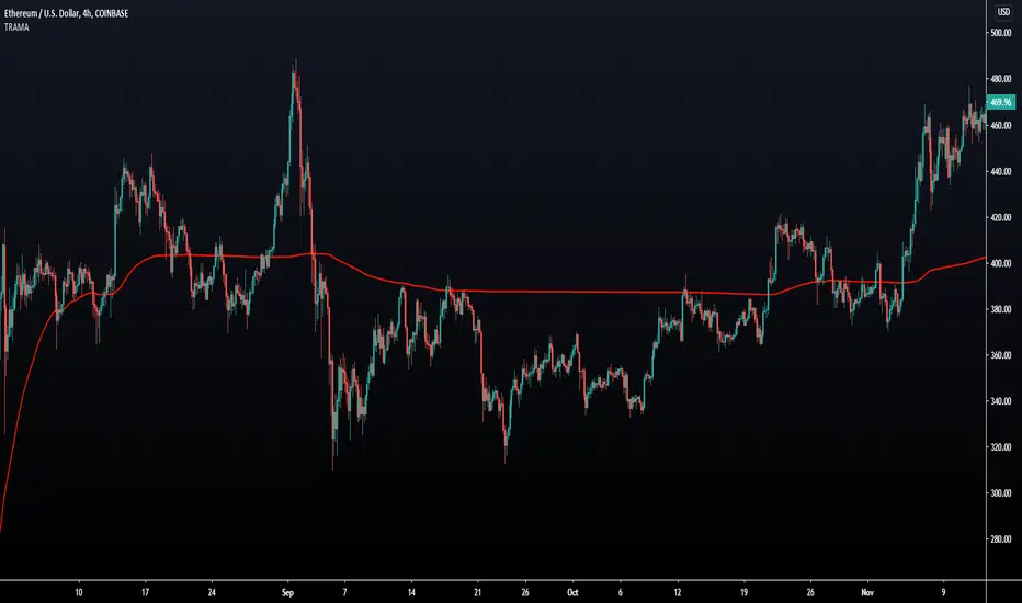
Trend Regularity Adaptive Moving Average [LuxAlgo]The following moving average adapt to the average number of highest high/lowest low made over a specific period, thus adapting to trend strength. Interesting results can be obtained when using the moving average in a MA crossover system or as a trailing support/resistance.
Settings
Length : Period of the indicator, with higher values returning smoother results.
Src : Source input of the indicator.
Usage
The trend regularity adaptive moving average (TRAMA) can be used like most moving averages, with the advantage of being smoother during ranging markets.
Notice how the moving closer to the price the longer a trend last, such effect can be practical to have early entry points when using the moving average in a MA crossover system, such effect is due to the increasing number of average highest high/lowest low made during longer trends. Note that in the case of a significant uptrend followed by a downtrend, the moving average might penalize the start of the downtrend (and vice versa).
The moving average can also act as an interesting trailing support/resistance.
Details
The moving average is calculated using exponential averaging, using as smoothing factor the squared simple moving average of the number of highest high/lowest low previously made, highest high/lowest low are calculated using rolling maximums/minimums.
Using higher values of length will return fewer highest high/lowest low which explains why the moving average is smoother for higher length values. Squaring allows the moving average to penalize lower values, thus appearing more stationary during ranging markets, it also allows to have some consistency regarding the length setting.
🧙 this moving average would not be possible without the existence of corn syrup 🦎
A Useful MA Weighting Function For Controlling Lag & SmoothnessSo far the most widely used moving average with an adjustable weighting function is the Arnaud Legoux moving average (ALMA), who uses a Gaussian function as weighting function. Adjustable weighting functions are useful since they allow us to control characteristics of the moving average such as lag and smoothness.
The following moving average has a simple adjustable weighting function that allows the user to have control over the lag and smoothness of the moving average, we will see that it can also be used to get both an SMA and WMA.
A high-resolution gradient is also used to color the moving average, makes it fun to watch, the plot transition between 200 colors, would be tedious to make but everything was made possible using a custom R script, I only needed to copy and paste the R console output in the Pine editor.
Settings
length : Period of the moving average
-Lag : Setting decreasing the lag of the moving average
+Lag : Setting increasing the lag of the moving average
Estimating Existing Moving Averages
The weighting function of this moving average is derived from the calculation of the beta distribution, advantages of such distribution is that unlike a lot of PDF, the beta distribution is defined within a specific range of values (0,1). Parameters alpha and beta controls the shape of the distribution, with alpha introducing negative skewness and beta introducing positive skewness, while higher values of alpha and beta increase kurtosis.
Here -Lag is directly associated to beta while +Lag is associated with alpha . When alpha = beta = 1 the distribution is uniform, and as such can be used to compute a simple moving average.
Moving average with -Lag = +Lag = 1 , its impulse response is shown below.
It is also possible to get a WMA by increasing -Lag , thus having -Lag = 2 and +Lag = 1 .
Using values of -Lag and +Lag equal to each other allows us to get a symmetrical impulse response, increasing these two values controls the heaviness of the tails of the impulse response.
Here -Lag = +Lag = 3 , note that when the impulse response of a moving average is symmetrical its lag is equal to (length-1)/2 .
As for the gradient, the color is determined by the value of an RSI using the moving average as input.
I don't promise anything but I will try to respond to your comments

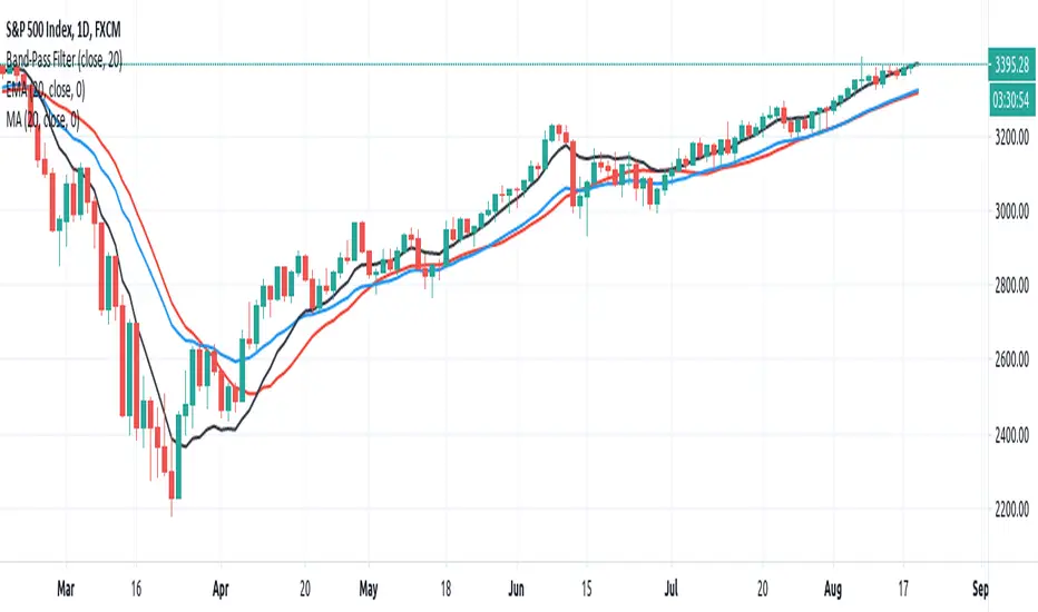
Band-Pass FilterJust a clean script that can be applied on top of other indicators/sources or you can take the function out of the source and use it in other scripts.
The idea for this was taken from www.pinecoders.com except I am utilizing an EMA instead of SMA. Simply put, we are combining a low-pass filter (moving average) with a high-pass filter (smoothed difference between the source and moving average). The result is a filter/moving average that provides a great combination of minimizing noise while still reacting strongly to price and trend changes.
I like to use this filter in place of other MAs in Pine Scripts to smooth my data. So instead of doing something like sma(stochastic,5) I can easily plug in bp(stochastic,5). It works just fine for your primary moving averages against price as well.
Shapeshifting Moving Average - Switching From Low-Lag To SmoothThe term "shapeshifting" is more appropriate when used with something with a shape that isn't supposed to change, this is not the case of a moving average whose shape can be altered by the length setting or even by an external factor in the case of adaptive moving averages, but i'll stick with it since it describe the purpose of the proposed moving average pretty well.
In the case of moving averages based on convolution, their properties are fully described by the moving average kernel ( set of weights ), smooth moving averages tend to have a symmetrical bell shaped kernel, while low lag moving averages have negative weights. One of the few moving averages that would let the user alter the shape of its kernel is the Arnaud Legoux moving average, which convolve the input signal with a parametric gaussian function in which the center and width can be changed by the user, however this moving average is not a low-lagging one, as the weights don't include negative values.
Other moving averages where the user can change the kernel from user settings where already presented, i posted a lot of them, but they only focused on letting the user decrease or increase the lag of the moving average, and didn't included specific parameters controlling its smoothness. This is why the shapeshifting moving average is proposed, this parametric moving average will let the user switch from a smooth moving average to a low-lagging one while controlling the amount of lag of the moving average.
Settings/Kernel Interaction
Note that it could be possible to design a specific kernel function in order to provide a more efficient approach to today goal, but the original indicator was a simple low-lag moving average based on a modification of the second derivative of the arc tangent function and because i judged the indicator a bit boring i decided to include this parametric particularity.
As said the moving average "kernel", who refer to the set of weights used by the moving average, is based on a modification of the second derivative of the arc tangent function, the arc tangent function has a "S" shaped curve, "S" shaped functions are called sigmoid functions, the first derivative of a sigmoid function is bell shaped, which is extremely nice in order to design smooth moving averages, the second derivative of a sigmoid function produce a "sinusoid" like shape ( i don't have english words to describe such shape, let me know if you have an idea ) and is great to design bandpass filters.
We modify this 2nd derivative in order to have a decreasing function with negative values near the end, and we end up with:
The function is parametric, and the user can change it ( thus changing the properties of the moving average ) by using the settings, for example an higher power value would reduce the lag of the moving average while increasing overshoots. When power < 3 the moving average can act as a slow moving average in a moving average crossover system, as weights would not include negative values.
Here power = 0 and length = 50. The shapeshifting moving average can approximate a simple moving average with very low power values, as this would make the kernel approximate a rectangular function, however this is only a curiosity and not something you should do.
As A Smooth Moving Average
“So smooth, and so tranquil. It doesn't get any quieter than this”
A smooth moving average kernel should be : symmetrical, not to width and not to sharp, bell shaped curve are often appropriates, the proposed moving average kernel can be symmetrical and can return extremely smooth results. I will use the Blackman filter as comparison.
The smooth version of the moving average can be used when the "smooth" setting is selected. Here power can only be an even number, if power is odd, power will be equal to the nearest lowest even number. When power = 0, the kernel is simply a parabola:
More smoothness can be achieved by using power = 2
In red the shapeshifting moving average, in green a Blackman filter of both length = 100. Higher values of power will create lower negative values near the border of the kernel shape, this often allow to retain information about the peaks and valleys in the input signal. Power = 6 approximate the Blackman filter pretty well.
Conclusion
A moving average using a modification of the 2nd derivative of the arc tangent function as kernel has been presented, the kernel is parametric and allow the user to switch from a low-lag moving average where the lag can be increased/decreased to a really smooth moving average.
As you can see once you get familiar with a function shape, you can know what would be the characteristics of a moving average using it as kernel, this is where you start getting intimate with moving averages.
On a side note, have you noticed that the views counter in posted ideas/indicators has been removed ? This is truly a marvelous idea don't you think ?
Thanks for reading !

Right Sided Ricker Moving Average And The Gaussian DerivativesIn general gaussian related indicators are built by using the gaussian function in one way or another, for example a gaussian filter is built by using a truncated gaussian function as filter kernel (kernel refer to the set weights) and has many great properties, note that i say truncated because the gaussian function is not supposed to be finite. In general the gaussian function is represented by a symmetrical bell shaped curve, however the gaussian function is parametric, and the user might adjust the position of the peak as well as the width of the curve, an indicator using this parametric approach is the Arnaud Legoux moving average (ALMA) who posses a length parameter controlling the filter length, a peak parameter controlling the position of the peak of the gaussian function as well as a width parameter, those parameters can increase/decrease the lag and smoothness of the moving average output.
However what about the derivatives of the gaussian function ? We don't talk much about them and thats a pity because they are extremely interesting and have many great properties as well, therefore in this post i'll present a low lag moving average based on the modification of the 2nd order derivative of the gaussian function, i believe this post will be extremely informative and i hope you will enjoy reading it, if you are not a math person you can skip the introduction on gaussian derivatives and their properties used as filter kernel.
Gaussian Derivatives And The Ricker Wavelet
The notion of derivative is continuous, so we will stick with the term discrete derivative instead, which just refer to the rate of change in the function, we have a change function in pinescript, and we will be using it to show an approximation of the gaussian function derivatives.
Earlier i used the term 2nd order derivative, here the derivative order refer to the order of differentiation, that is the number of time we apply the change function. For example the 0 (zeroth) order derivative mean no differentiation, the 1st order derivative mean we use differentiation 1 time, that is change(f) , 2nd order mean we use differentiation 2 times, that is change(change(f)) , derivates based on multiple differentiation are called "higher derivative". It will be easier to show a graphic :
Here we can see a normal gaussian function in blue, its scaled 1st order derivative in orange, and its scaled 2nd derivative in green, note that i use scaled because i used multiplication in order for you to see each curve, else it would have been less easy to observe them. The number of time a gaussian function derivative cross 0 is based on the order of differentiation, that is 2nd order = the function crossing 0 two times.
Now we can explain what is the Ricker wavelet, the Ricker wavelet is just the normalized 2nd order derivative of a gaussian function with inverted sign, and unlike the gaussian function the only thing you can change is the width parameter. The formula of the Ricker wavelet is show'n here en.wikipedia.org , where sigma is the width parameter.
The Ricker wavelet has this look :
Because she is shaped like a sombrero the Ricker wavelet is also called "mexican hat wavelet", now what would happen if we used a Ricker wavelet as filter kernel ? The response is that we would end-up with a bandpass filter, in fact the derivatives of the gaussian function would all give the kernel of a bandpass filter, with higher order derivatives making the frequency response of the filter approximate a symmetrical gaussian function, if i recall a filter using the first order derivative of a gaussian function would give a frequency response that is left skewed, this skewness is removed when using higher order derivatives.
The Indicator
I didn't wanted to make a bandpass filter, as lately i'am more interested in low-lag filters, so how can we use the Ricker wavelet to make a low-lag low-pass filter ? The response is by taking the right side of the Ricker wavelet, and since values of the wavelets are negatives near the border we know that the filter passband is non-monotonic, that is we know that the filter will have low-lag as frequencies in the passband will be amplified.
So taking the right side of the Ricker wavelet only mean that t has to be greater than 0 and linearly increasing, thats easy, however the width parameter can be tricky to use, this was already the case with ALMA, so how can we work with it ? First it can be seen that values of width needs to be adjusted based on the filter length.
In red width = 14, in green width = 5. We can see that an higher values of width would give really low weights, when the number of negative weights is too important the filter can have a negative group delay thus becoming predictive, this simply mean that the overshoots/undershoots will be crazy wild and that a great fit will be impossible.
Here two moving averages using the previous described kernels, they don't fit the price well at all ! In order to fix this we can simply define width as a function of the filter length, therefore the parameter "Percentage Width" was introduced, and simply set the width of the Ricker wavelet as p percent of the filter length. Lower values of percent width reduce the lag of the moving average, but lets see precisely how this parameter influence the filter output :
Here the filter length is equal to 100, and the percent width is equal to 60, the fit is quite great, lower values of percent width will increase overshoots, in fact the filter become predictive once the percent width is equal or lower to 50.
Here the percent width is equal to 50. Higher values of percent width reduce the overshoots, and a value of 100 return a filter with no overshoots that is suited to act as a lagging moving average.
Above percent width is set to 100. In order to make use of the predictive side of the filter, it would be great to introduce a forecast option, however this require to find the best forecast horizon period based on length and width, this is no easy task.
Finally lets estimate a least squares moving average with the proposed moving average, you know me...a percent width set to 63 will return a relatively good estimate of the LSMA.
LSMA in green and the proposed moving in red with percent width = 63 and both length = 100.
Conclusion
A new low-lag moving average using a right sided Ricker wavelet as filter kernel has been introduced, we have also seen some properties of gaussian derivatives. You can see that lately i published more moving averages where the user can adjust certain properties of the filter kernel such as curve width for example, if you like those moving averages you can check the Parametric Corrective Linear Moving Averages indicator published last month :
I don't exclude working with pure forms of gaussian derivatives in the future, as i didn't published much oscillators lately.
Thx for reading !

Grover Llorens Cycle Oscillator [alexgrover & Lucía Llorens]Cycles represent relatively smooth fluctuations with mean 0 and of varying period and amplitude, their estimation using technical indicators has always been a major task. In the additive model of price, the cycle is a component :
Price = Trend + Cycle + Noise
Based on this model we can deduce that :
Cycle = Price - Trend - Noise
The indicators specialized on the estimation of cycles are oscillators, some like bandpass filters aim to return a correct estimate of the cycles, while others might only show a deformation of them, this can be done in order to maximize the visualization of the cycles.
Today an oscillator who aim to maximize the visualization of the cycles is presented, the oscillator is based on the difference between the price and the previously proposed Grover Llorens activator indicator. A relative strength index is then applied to this difference in order to minimize the change of amplitude in the cycles.
The Indicator
The indicator include the length and mult settings used by the Grover Llorens activator. Length control the rate of convergence of the activator, lower values of length will output cycles of a faster period.
here length = 50
Mult is responsible for maximizing the visualization of the cycles, low values of mult will return a less cyclical output.
Here mult = 1
Finally you can smooth the indicator output if you want (smooth by default), you can uncheck the option if you want a noisy output.
The smoothing amount is also linked with the period of the rsi.
Here the smoothing amount = 100.
Conclusion
An oscillator based on the recently posted Grover Llorens activator has been proposed. The oscillator aim to maximize the visualization of cycles.
Maximizing the visualization of cycles don't comes with no cost, the indicator output can be uncorrelated with the actual cycles or can return cycles that are not present in the price. Other problems arises from the indicator settings, because cycles are of a time-varying periods it isn't optimal to use fixed length oscillators for their estimation.
Thanks for reading !
If my work has ever been of use to you you can donate, addresses on my signature :)
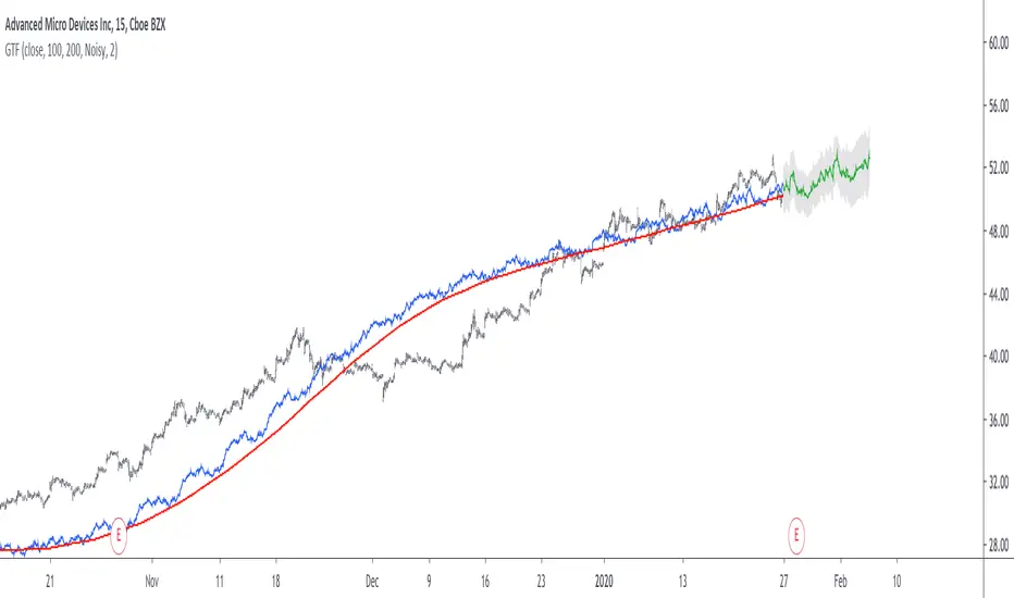
Grand Trend Forecasting - A Simple And Original Approach Today we'll link time series forecasting with signal processing in order to provide an original and funny trend forecasting method, the post share lot of information, if you just want to see how to use the indicator then go to the section "Using The Indicator".
Time series forecasting is an area dealing with the prediction of future values of a series by using a specific model, the model is the main tool that is used for forecasting, and is often an expression based on a set of predictor terms and parameters, for example the linear regression (model) is a 1st order polynomial (expression) using 2 parameters and a predictor variable ax + b . Today we won't be using the linear regression nor the LSMA.
In time series analysis we can describe the time series with a model, in the case of the closing price a simple model could be as follows :
Price = Trend + Cycles + Noise
The variables of the model are the components, such model is additive since we add the component with each others, we should be familiar with each components of the model, the trend represent a simple long term variation of high amplitude, the cycles are periodic fluctuations centered around 0 of varying period and amplitude, the noise component represent shorter term irregular variations with mean 0.
As a trader we are mostly interested by the cycles and the trend, altho the cycles are relatively more technical to trade and can constitute parasitic fluctuations (think about retracements in a trend affecting your trend indicator, causing potential false signals).
If you are curious, in signal processing combining components has a specific name, "synthesis" , here we are dealing with additive synthesis, other type of synthesis are more specific to audio processing and are relatively more complex, but could be used in technical analysis.
So what to do with our components ? If we want to trade the trend, we should estimate right ? Estimating the trend component involve removing the cycle and noise component from the price, if you have read stuff about filters you should know where i'am going, yep, we should use filters, in the case of keeping the trend we can use a simple moving average of relatively high period, and here we go.
However the lag problem, which is recurrent, come back again, we end up with information easier to interpret (here the trend, which is a simple fluctuation such as a line or other smooth curve) at the cost of decision timing, that is unfortunate but as i said the information, here the moving average output, is relatively simple, and could be easily forecasted right ? If you plot a moving average of high period it would be easier for you to forecast its future values. And thats what we aim to do today, provide an estimate of the trend that should be easy to forecast, and should fit to the price relatively well in order to produce forecast that could determine the position of future closing prices observations.
Estimating And Forecasting The Trend
The parameter of the indicator dealing with the estimation of the trend is length , with higher values of length attenuating the cycle and noise component in the price, note however that high values of length can return a really long term trend unlike a simple moving average, so a small value of length, 14 for example can still produce relatively correct estimate of trend.
here length = 14.
The rough estimate of the trend is t in the code, and is an IIR filter, that is, it is based on recursion. Now i'll pass on the filter design explanation but in short, weights are constants, with higher weights allocated to the previous length values of the filter, you can see on the code that the first part of t is similar to an exponential moving average with :
t(n) = 0.9t(n-length) + 0.1*Price
However while the EMA only use the precedent value for the recursion, here we use the precedent length value, this would just output a noisy and really slow output, therefore in order to create a better fit we add : 0.9*(t(n-length) - t(n-2length)) , and this create the rough trend estimate that you can see in blue. On the parameters, 0.9 is used since it gives the best estimate in my opinion, higher values would create more periodic output and lower values would just create a rougher output.
The blue line still contain a residual of the cycle/noise component, this is why it is smoothed with a simple moving average of period length. If you are curious, a filter estimating the trend but still containing noisy fluctuations is called "Notch" filter, such filter would depending on the cutoff remove/attenuate mid term cyclic fluctuations while preserving the trend and the noise, its the opposite of a bandpass filter.
In order to forecast values, we simply sum our trend estimate with the trend estimate change with period equal to the forecasting horizon period, this is a really really simple forecasting method, but it can produce decent results, it can also allows the forecast to start from the last point of the trend estimate.
Using The Indicator
We explained the length parameter in the precedent section, src is the input series which the trend is estimated, forecast determine the forecasting horizon, recommend values for forecast should be equal to length, length/2 or length*2, altho i strongly recommend length.
here length and forecast are both equal to 14 .
The corrective parameter affect the trend estimate, it reduce the overshoot and can led to a curve that might fit better to the price.
The indicator with the non corrective version above, and the corrective one below.
The source parameter determine the source of the forecast, when "Noisy" is selected the source is the blue line, and produce a noisy forecast, when "Smooth" is selected the source is the moving average of t , this create a smoother forecast.
The width interval control...the width of the intervals, they can be seen above and under the forecast plot, they are constructed by adding/subtracting the forecast with the forecast moving average absolute error with respect to the price. Prediction intervals are often associated with a probability (determining the probability of future values being between the interval) here we can't determine such probability with accuracy, this require (i think) an analysis of the forecasting distribution as well as assumptions on the distribution of the forecasting error.
Finally it is possible to see historical forecasts, that is, forecasts previously generated by checking the "Show Historical Forecasts" option.
Examples
Good forecasts mostly occur when the price is close to the trend estimate, this include the following highlighted periods on AMD 15TF with default settings :
We can see the same thing at the end of EURUSD :
However we can't always obtain suitable fits, here it is isn't sufficient on BTCUSD :
We can see wide intervals, we could change length or use the corrective option to get better results, another option is to use a log scale.
We will end the examples with the log SPX, who posses a linear trend, so for example a linear model such as a linear regression would be really adapted, lets see how the indicator perform :
Not a great fit, we could try to use an higher length value and use "Smooth" :
Most recent fits are quite decent.
Conclusions
A forecasting indicator has been presented in this post. The indicator use an original approach toward estimating the trend component in the closing price. Of course i should have given statistics related to the forecasting error, however such analysis is worth doing with better methods and in more advanced environment allowing for optimization.
But we have learned some stuff related to signal processing as well as time series analysis, seeing a time series as the sum of various components is really helpful when it comes to make sense of chaotic and noisy series and is a basic topic in time series analysis.
You can see that in this new year i work harder on the visual of my indicators without trying to fall in the label addict trap, something that i wasn't really doing before, let me know what do you think of it.
Thanks for reading !
Uber Moving Averages [UTS]Uber Moving Averages are four highly customisable moving averages to complement your technical analysis.
The optional trend direction visualisation makes it a powerful tool for trend weighted analysis.
Moving Averages
16 different Moving Averages are at your disposal.
Trend Visualisation
If the predominant trend direction is DOWN the moving average is painted red. If the trend direction is UP the moving average is painted in green.
Windowed Volume Weighted Moving AverageIntroduction
The concept of windowing was briefly introduced in the Blackman filter post, however windowing is more than just some window functions, and isn't exclusively used in filter design.
Today we will use windowing with the volume weighted moving average, a moving average that weight the price with volume in order to be more reactive when volume is high, that is the moving average is more reactive when the market is more active. The use of windowing in the vwma allow to enhance its performance in the frequency domain which result in a smoother output.
Note that i made a similar indicator long ago, but at that time I was not great at all with math and pinescript in general and the indicator was therefore wrong, i want to remind to the community that i'am not a professional, only an enthusiast, I never claimed to be a master coder and i'am totally open to receive criticism, if I sounded like bragging in the past I apologize, at 20 years old it is still easy to act like a kid, the information contained in my posts is only shared in order to help others but also myself, since sharing is also a way to learn more effectively. That said lets go with the indicator.
Windowing
Windowing consist on applying a window function to a signal, by applying i mostly talk about multiplying, this process is mostly used with windowed sinc filters in order to reduce ripples in the pass/stop band, but can be used with any kind of filters in order to have better frequency domain performance, the only thing we need to do is to multiply the filter weights by a window function.
In order to understand windowing it is useful to visualize this process and understand spectral leakage. Remember that we can describe a signal as the sum of sine/cosine waves of different frequencies, amplitude and phase, leakage is an effect that appear with signals having discontinuities, that is when a signal non periodic.
This figure show a non periodic sine wave of frequency 0.1, a non periodic signal will have is last sample value different from its first sample value, if we where to do its fourier transform we wouldn't end up with a single bin at 0.1 but with more bins, this is spectral leakage, the discontinuities in the signal create additional frequency components. In order to reduce leakage we must make the signal approximately periodic, this is done by making use of window functions.
A window function is symmetric and relatively smooth, all we have to do is to multiply our first non periodic signal with the window function.
We end up with the following windowed signal :
The signal is approximately periodic and leakage has been reduced. Now that we have seen that, it might be useful to see why it is useful in filters.
Remember that the Fourier transform of the filter weights gives us its frequency response, if our weights introduce leakage we end up with ripples, so windowing the filter weights might help reduce the ripples in the frequency response, which result in a smoother filter output.
Volume Weighted Moving Average
A volume weighted moving average is a FIR filter who use volume as filter kernel, therefore the frequency response of this filter always change, it is therefore not wrong to qualify the vwma as an adaptive moving average. Higher volume mean higher weighting of the current closing price value, which therefore produce a more reactive output.
However the smoothness of the moving average is relatively poor.
Windowed Volume Weighted Moving Average
The proposed moving average has a length setting who control the moving average period, and various options that we will describe below. The first option is the type of window, there are many windows, certains more complex than others, here 3 windows are proposed, the famous Blackman window, the Bartlett, and finally the Hanning window, they provide each different level of smoothness. lets compare our moving average with period 100 with a vwma of the same period.
Our moving average in red, and the vwma in blue. As you can see the results are smoother.
The power parameter is used in order to give an even higher weighting to closing prices with high volume, this create a more boxy output. Below is a comparison with a vwma in blue and a powered vwma in red with power = 2 without windowing :
We can then apply a window, here i will choose the Blackman window :
Conclusion
A new moving average based on windowed volume weighting has been proposed. The result are smoother which might therefore reduce whipsaw trades. I wish i could have explained things better, unfortunately windowing isn't something i use much, i wanted to post this moving average earlier this year.
I will be off in France for 1 week, my flight is tomorrow in the morning, therefore i don't think i'll have the possibility to make other posts this year. I want to profit from this occasion to review my year in tradingview.
Many indicators have been posted, some being extremely bad and others really interesting, this year introduced my attempts on estimating the lsma efficiently, the linear channels, an attempt on making lines and remain the first indicator from the v4 i posted if i'am right. Then came the efficient auto-line, who gained some popularity quite fast. Then finally the %G oscillator and the recursive bands where posted, and remain some of the favorites indicators i made. I also wanted to leave this year due to studies, that i totally abandoned, i'am thankful that i chosen to stay.
I also want to express my apologies to any member that i could have offended, i think that i'am not a mean person but i certainly not contest the fact that i'am clumsy, even in my work, however my clumsiness is far greater when it comes to interact with other peoples or a group of peoples, i don't want to hurt anyone, if i made anything that made you feel bad then i'am sincerely sorry, and hope we can start this new year from 0.
Finally i thank the tradingview community for their interest and curiosity, i thank all the great coders who work on making pinescript a better scripting language, i also thank the tradingview staff for their work this year. I wish you all a merry christmas, and an happy new year.
Thanks for reading.
Blackman Filter - The Smoother The BetterIntroduction
Who doesn't like smooth things? I'd like a smooth market price for christmas! But i can't get it, instead its so noisy...so you apply a filter to smooth it, such filters are called low-pass filters, they smooth and its great but they have lag, so nobody really use them, but they are pretty to look at.
Its on a childish note that i will introduce this indicator, so what it is all about? I propose a new FIR filter using a blackman function as filter kernel for financial time-series smoothing, do you prefer the childish tone ? Fear not its surprisingly easy!
The Blackman Function
The blackman function look like a bell shaped curve, look:
The blackman function will produce such curve. This function is called a cosine sum function because she is based on the sum of cosine functions, here only 2.
0.42 - 0.5 * cos(2 * pi * k) + 0.08 * cos(4 * pi * k)
Originally you use this function for windowing , what does it means? In signal processing you have a function called sync function , if you use this function as filter kernel you would get the ideal frequency domain response filter, sometime called brickwall filter, it would be extremely smooth.
Above the optimal low pass filter frequency response.
However the sync function has no ending values and goes on forever, therefore we can't use it for convolution, expect if we apply windowing. Filters using windowing are called windowed-sinc filters, i will describe the procedure below :
1 - Create a sync function = sin(pi*n)/(pi*n)
2 - Truncate it = I only keep the first length points of the sync function.
This create a abrupt end, the frequency of a filter using step 1 as kernel would contain ripples in the pass band and stop band, this is bad! The frequency response would look like this :
3 - I multiply my values of step 2 by a window function, it can the blackman window, i no longer have an abrupt end, its smooth!
The frequency response of the filter using this kernel would no longer have ripples! This is the power of windowing functions.
Here we are not using such thing, but we could in the future. Here instead we use the blackman function as filter kernel, because this function is bell shaped this mean that the filter will certainly be smooth (symmetrical weighting is a rule of thumb for kernels when we want really smooth filters).
The Filter
This filter is quite smooth, unlike the gaussian filter this filter give less weights to recent and past values, this is because the blackman function has fatter tails than the gaussian one. I could make a comparison of both, however they are quite alike, if you often use a gaussian filter its up to you to decide which one you prefer.
The filter can do a better job than the moving average when it comes to preserve the frequency components that constitute the cycles/trend.
We can see that the filter has a greater performance when it comes to keep the shape of the market price, thus it has a slightly better fit.
Conclusion
Ok so in this post you learned a bit about the sync function and windowing, those are basic subjects in signal processing, they allow us to approximate the filter with the ideal frequency response, i also showed you that those windowing function could be used as kernel and that they where pretty smooth on their own, there are many others, but the one i prefer is the blackman windowing function.
I know what you are thinking, "we want trailing stops, alerts, colors, arrows!", and i understand you pal, but sometimes its cool to take a break from all this stuff. However i can tell that i'am working on a side project that aim to estimate rolling maximum/minimum as fast as possible, any experiments will be published here, and i can ensure you that those indicators will make your day quite brighter, we will see that soon.
I hope you learned something from this post! I'am a bit tired (look i'am disappearing !)
Thanks for reading !
