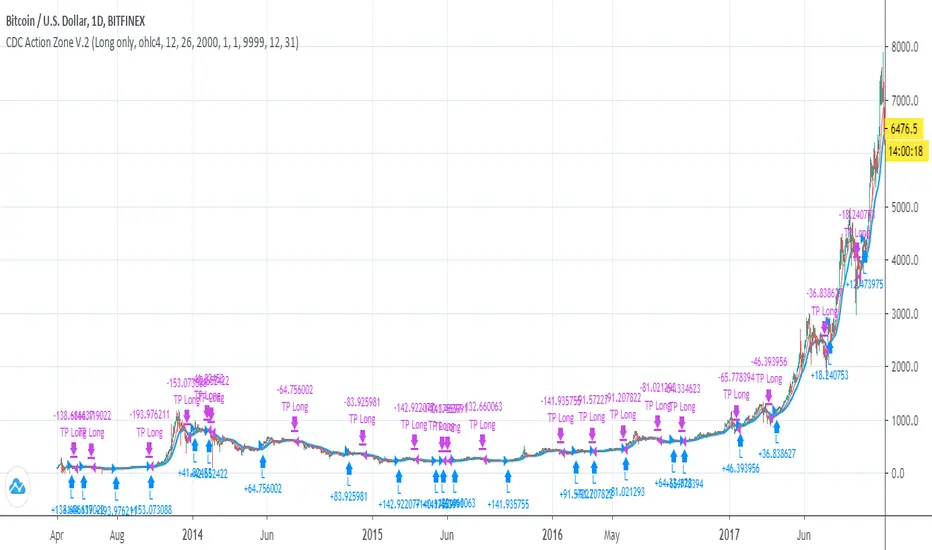
CDC Action Zone V.2 Strategy BacktestPublished for backtest purpose
All credit to : CDC Action Zone V.2 by piriya33
จัดทำขึ้นเพื่อการดูผล Backtest เขียวซื้อแดงขาย
ตัวสคริปท์มีการเพิ่ม
- Strategy Long/Short/Both // ปรับได้ใน Setting
- Back test range // ปรับได้ใน Setting
Cari dalam skrip untuk "zone"
Chop Zone Strategy - Buy OnlyUses build-in indicator "Chop Zone" which measures angle of EMA-34.
Buy when there are 3 consecutive turquoise bar.
Close when there are 3 consecutive non-turquoise bar.


16. SMC Strategy with SL - low TimeframeOverview
The "SMC Strategy with SL - low Timeframe" is a comprehensive trading strategy that uses key concepts from Smart Money Theory to identify favorable areas in the market for buying or selling. This strategy takes advantage of price imbalances, support and resistance zones, and swing highs/lows to generate high-probability trade signals.
The key features of this strategy include:
Swing High/Low Analysis: Used to determine the Premium, Equilibrium, and Discount Zones.
Order Block Integration: An added layer of confluence to identify valid buy and sell signals.
Trend Direction Confirmation: Using a Simple Moving Average (SMA) to determine the overall trend.
Entry and Exit Rules: Based on price position relative to key zones and moving average, along with optional stop-loss and take-profit levels.
Detailed Description
Swing High and Swing Low Analysis
The script calculates Swing High and Swing Low based on the most recent price highs and lows over a specified look-back period (swingHighLength and swingLowLength, set to 8 by default).
It then derives the Premium, Equilibrium, and Discount Zones:
Premium Zone: Represents potential resistance, calculated based on recent swing highs.
Discount Zone: Represents potential support, calculated based on recent swing lows.
Equilibrium: The midpoint between Swing High and Swing Low, dividing the price range into Premium (above equilibrium) and Discount (below equilibrium) areas.
Zone Visualization
The strategy plots the Premium Zone (resistance) in red, the Discount Zone (support) in green, and the Equilibrium level in blue on the chart. This helps visually assess the current price relative to these important areas.
Simple Moving Average (SMA)
A 50-period Simple Moving Average (SMA) is added to help identify the trend direction.
Buy signals are valid only if the price is above the SMA, indicating an uptrend.
Sell signals are valid only if the price is below the SMA, indicating a downtrend.
Entry Rules
The script generates buy or sell signals when certain conditions are met:
A buy signal is triggered when:
Price is below the Equilibrium and within the Discount Zone.
Price is above the SMA.
The buy signal is further confirmed by the presence of an Order Block (recent lowest price area).
A sell signal is triggered when:
Price is above the Equilibrium and within the Premium Zone.
Price is below the SMA.
The sell signal is further confirmed by the presence of an Order Block (recent highest price area).
Order Block
The strategy defines Order Blocks as recent highs and lows within a look-back period (orderBlockLength set to 20 by default).
These blocks represent areas where large players (smart money) have historically been active, increasing the probability of the price reacting in these areas again.
Trade Management and Trade Direction
The user can set Trade Direction to either "Long Only," "Short Only," or "Both." This allows the strategy to adapt based on market conditions or trading preferences.
Based on the Trade Direction, the strategy either:
Closes open trades that are against new signals.
Allows only specific directional trades (either long or short).
Stop-loss levels are defined based on a fixed percentage (stop_loss_percent), which helps to manage risk and minimize losses.
Exit Rules
The strategy uses stop-loss levels for risk management.
A stop-loss price is set at a fixed percentage below the entry price for long positions or above the entry price for short positions.
When the price hits the defined stop-loss level, the trade is closed.
Liquidity Zones
The script identifies recent Swing Highs and Lows as potential liquidity zones. These are levels where price could react strongly, as they represent areas of interest for large traders.
The liquidity zones are plotted as crosses on the chart, marking areas where price may encounter significant buying or selling pressure.
Visual Feedback
The script uses visual markers (green for buy signals and red for sell signals) to indicate potential entries on the chart.
It also plots liquidity zones to help traders identify areas where stop hunts and liquidity grabs might occur.
Monthly Performance Dashboard
The script includes a performance tracking feature that displays monthly profit and loss metrics on the chart.
This dashboard allows the trader to see a visual representation of trading performance over time, providing insights into profitability and consistency.
The table shows profit or loss for each month and year, allowing the user to track the overall success of the strategy.
Key Benefits
Smart Money Concepts (SMC): This strategy incorporates SMC principles like order blocks and liquidity zones, which are used by institutional traders to determine potential market moves.
Zone Analysis: The use of Premium, Discount, and Equilibrium zones provides a solid framework for determining where to enter and exit trades based on price discounts or premiums.
Confluence: Signals are not taken in isolation. They are confirmed by factors like trend direction (SMA) and order blocks, providing greater trade accuracy.
Risk Management: By integrating stop-loss functionality, traders can manage their risks effectively.
Visual Performance Metrics: The monthly and yearly performance dashboard gives valuable feedback on how well the strategy has performed historically.
Practical Use
Buy in Discount Zone: Traders would be looking to buy when the price is discounted relative to its recent range and is above the SMA, indicating an overall uptrend.
Sell in Premium Zone: Conversely, traders would be looking to sell when the price is at a premium relative to its recent range and below the SMA, indicating an overall downtrend.
Order Block Confirmation: Ensures that buying or selling is supported by historical price behavior at significant levels, providing confidence that the market is likely to react at these areas.
This strategy is designed to help traders take advantage of price inefficiencies and areas where institutional traders are likely to be active, increasing the odds of successful trades. By leveraging Smart Money concepts and strong technical confluence, it aims to provide high-probability trade setups.

ATH대비 지정하락률에 도착 시 매수 - 장기홀딩 선물 전략(ATH Drawdown Re-Buy Long Only)본 스크립트는 과거 하락 데이터를 이용하여, 정해진 하락 %가 발생하는 경우 자기 자본의 정해진 %만큼을 진입하게 설계되어진 스트레티지입니다.
레버리지를 사용할 수 있으며 기본적으로 셋팅해둔 값이 내장되어있습니다.(자유롭게 바꿔서 쓰시면 됩니다.) 추가적으로 2번의 진입 외에도 다른 진입 기준, 진입 %를 설정하실 수 있으며 - ChatGPT에게 요청하면 수정해줄 것입니다.
실제 사용용도로는 KillSwitch 기능을 꺼주세요. 바 돋보기 기능을 켜주세요.
ATH Drawdown Re-Buy Long Only 전략 설명
1. 전략 개요
ATH Drawdown Re-Buy Long Only 전략은 자산의 역대 최고가(ATH, All-Time High)를 기준으로 한 하락폭(드로우다운)을 활용하여,
특정 구간마다 단계적으로 롱 포지션을 구축하는 자동 재매수(Long Only) 전략입니다.
본 전략은 다음과 같은 목적을 가지고 설계되었습니다.
급격한 조정 구간에서 체계적인 분할 매수 및 레버리지 활용
ATH를 기준으로 한 명확한 진입 규칙 제공
실시간으로
평단가
레버리지
청산가 추정
계좌 MDD
수익률
등을 시각적으로 제공하여 리스크와 포지션 상태를 직관적으로 확인할 수 있도록 지원
※ 본 전략은 교육·연구·백테스트 용도로 제공되며,
어떠한 형태의 투자 권유 또는 수익을 보장하지 않습니다.
2. 전략의 핵심 개념
2-1. ATH(역대 최고가) 기준 드로우다운
전략은 차트 상에서 항상 가장 높은 고가(High)를 ATH로 기록합니다.
새로운 고점이 형성될 때마다 ATH를 갱신하고, 해당 ATH를 기준으로 다음을 계산합니다.
현재 바의 저가(Low)가 ATH에서 몇 % 하락했는지
현재 바의 종가(Close)가 ATH에서 몇 % 하락했는지
그리고 사전에 설정한 두 개의 드로우다운 구간에서 매수를 수행합니다.
1차 진입 구간: ATH 대비 X% 하락 시
2차 진입 구간: ATH 대비 Y% 하락 시
각 구간은 ATH가 새로 갱신될 때마다 한 번씩만 작동하며,
새로운 ATH가 생성되면 다시 “1차 / 2차 진입 가능 상태”로 초기화됩니다.
2-2. 첫 포지션 100% / 300% 특수 규칙
이 전략의 중요한 특징은 **“첫 포지션 진입 시의 예외 규칙”**입니다.
전략이 현재 어떠한 포지션도 들고 있지 않은 상태에서
최초로 롱 포지션을 진입하는 시점(첫 포지션)에 대해:
기본적으로는 **자산의 100%**를 기준으로 포지션을 구축하지만,
만약 그 순간의 가격이 ATH 대비 설정값 이상(예: 약 –72.5% 이상 하락한 상황) 이라면
→ 자산의 300% 규모로 첫 포지션을 진입하도록 설계되어 있습니다.
이 규칙은 다음과 같이 동작합니다.
첫 진입이 1차 드로우다운 구간에서 발생하든,
첫 진입이 2차 드로우다운 구간에서 발생하든,
현재 하락폭이 설정된 기준 이상(예: –72.5% 이상) 이라면
→ “이 정도 하락이면 첫 진입부터 더 공격적으로 들어간다”는 의미로 300% 규모로 진입
그 이하의 하락폭이라면
→ 첫 진입은 100% 규모로 제한
즉, 전략은 다음 두 가지 모드로 동작합니다.
일반적인 상황의 첫 진입: 자산의 100%
심각한 드로우다운 구간에서의 첫 진입: 자산의 300%
이 특수 규칙은 깊은 하락에서는 공격적으로, 평소에는 상대적으로 보수적으로 진입하도록 설계된 것입니다.
3. 전략 동작 구조
3-1. 매수 조건
차트 상 High 기준으로 ATH를 추적합니다.
각 바마다 해당 ATH에서의 하락률을 계산합니다.
사용자가 설정한 두 개의 드로우다운 구간(예시):
1차 구간: 예를 들어 ATH – 50%
2차 구간: 예를 들어 ATH – 72.5%
각 구간에 대해 다음과 같은 조건을 확인합니다.
“이번 ATH 구간에서 아직 해당 구간 매수를 한 적이 없는 상태”이고,
현재 바의 저가(Low)가 해당 구간 가격 이하를 찍는 순간
→ 해당 바에서 매수 조건 충족으로 간주
실제 주문은:
해당 구간 가격에 맞춰 롱 포지션 진입(리밋/시장가 기반 시뮬레이션) 으로 처리됩니다.
3-2. ATH 갱신과 진입 기회 리셋
차트 상에서 새로운 고점(High)이 기존 ATH를 넘어서는 순간,
ATH가 갱신되고,
1차 / 2차 진입 여부를 나타내는 내부 플래그가 초기화됩니다.
이를 통해, 시장이 새로운 고점을 돌파해 나갈 때마다,
해당 구간에서 다시 한 번씩 1차·2차 드로우다운 진입 기회를 갖게 됩니다.
4. 포지션 사이징 및 레버리지
4-1. 계좌 자산(Equity) 기준 포지션 크기 결정
전략은 현재 계좌 자산을 다음과 같이 정의하여 사용합니다.
현재 자산 = 초기 자본 + 실현 손익 + 미실현 손익
각 진입 구간에서의 포지션 가치는 다음과 같이 결정됩니다.
1차 진입 구간:
“자산의 몇 %를 사용할지”를 설정값으로 입력
설정된 퍼센트를 계좌 자산에 곱한 뒤,
다시 전략 내 레버리지 배수(Leverage) 를 곱하여 실제 포지션 가치를 계산
2차 진입 구간:
동일한 방식으로, 독립된 퍼센트 설정값을 사용
즉, 포지션 가치는 다음과 같이 계산됩니다.
포지션 가치 = 현재 자산 × (해당 구간 설정 % / 100) × 레버리지 배수
그리고 이를 해당 구간의 진입 가격으로 나누어 실제 수량(토큰 단위) 를 산출합니다.
4-2. 첫 포지션의 예외 처리 (100% / 300%)
첫 포지션에 대해서는 위의 일반적인 퍼센트 설정 대신,
다음과 같은 고정 비율이 사용됩니다.
기본: 자산의 100% 규모로 첫 포지션 진입
단, 진입 시점의 ATH 대비 하락률이 설정값 이상(예: –72.5% 이상) 일 경우
→ 자산의 300% 규모로 첫 포지션 진입
이때 역시 다음 공식을 사용합니다.
포지션 가치 = 현재 자산 × (100% 또는 300%) × 레버리지
그리고 이를 가격으로 나누어 실제 진입 수량을 계산합니다.
이 규칙은:
첫 진입이 1차 구간이든 2차 구간이든 동일하게 적용되며,
“충분히 깊은 하락 구간에서는 첫 진입부터 더 크게,
평소에는 비교적 보수적으로” 라는 운용 철학을 반영합니다.
4-3. 실레버리지(Real Leverage)의 추적
전략은 각 바 단위로 다음을 추적합니다.
바가 시작할 때의 기존 포지션 크기
해당 바에서 새로 진입한 수량
이를 바탕으로, 진입이 발생한 시점에 다음을 계산합니다.
실제 레버리지 = (포지션 가치 / 현재 자산)
그리고 차트 상에 예를 들어:
Lev 2.53x 와 같은 형식의 레이블로 표시합니다.
이를 통해, 매수 시점마다 실제 계좌 레버리지가 어느 정도였는지를 직관적으로 확인할 수 있습니다.
5. 시각화 및 모니터링 요소
5-1. 차트 상 시각 요소
전략은 차트 위에 다음과 같은 정보를 직접 표시합니다.
ATH 라인
High 기준으로 계산된 역대 최고가를 주황색 선으로 표시
평단가(평균 진입가) 라인
현재 보유 포지션이 있을 때,
해당 포지션의 평균 진입가를 노란색 선으로 표시
추정 청산가(고정형 청산가) 라인
포지션 수량이 변화하는 시점을 감지하여,
당시의 평단가와 실제 레버리지를 이용해 근사적인 청산가를 계산
이를 빨간색 선으로 차트에 고정 표시
포지션이 없거나 레버리지가 1배 이하인 경우에는 청산가 라인을 제거
매수 마커 및 레이블
1차/2차 매수 조건이 충족될 때마다 해당 지점에 매수 마커를 표시
"Buy XX% @ 가격", "Lev XXx" 형태의 라벨로
진입 비율과 당시 레버리지를 함께 시각화
레이블의 위치는 설정에서 선택 가능:
바 아래 (Below Bar)
바 위 (Above Bar)
실제 가격 위치 (At Price)
5-2. 우측 상단 정보 테이블
차트 우측 상단에는 현재 계좌·포지션 상태를 요약한 정보 테이블이 표시됩니다.
대표적으로 다음 항목들이 포함됩니다.
Pos Qty (Token)
현재 보유 중인 포지션 수량(토큰 기준, 절대값 기준)
Pos Value (USDT)
현재 포지션의 시장 가치 (수량 × 현재 가격)
Leverage (Now)
현재 실레버리지 (포지션 가치 / 현재 자산)
DD from ATH (%)
현재 가격 기준, 최근 ATH에서의 하락률(%)
Avg Entry
현재 포지션의 평균 진입 가격
PnL (%)
현재 포지션 기준 미실현 손익률(%)
Max DD (Equity %)
전략 전체 기간 동안 기록된 계좌 기준 최대 손실(MDD, Max Drawdown)
Last Entry Price
가장 최근에 포지션을 추가로 진입한 직후의 평균 진입 가격
Last Entry Lev
위 “Last Entry Price” 시점에서의 실레버리지
Liq Price (Fixed)
위에서 설명한 고정형 추정 청산가
Return from Start (%)
전략 시작 시점(초기 자본) 대비 현재 계좌 자산의 총 수익률(%)
이 테이블을 통해 사용자는:
현재 계좌와 포지션의 상태
리스크 수준
누적 성과
를 직관적으로 파악할 수 있습니다.
6. 시간 필터 및 라벨 옵션
6-1. 전략 동작 기간 설정
전략은 옵션으로 특정 기간에만 전략을 동작시키는 시간 필터를 제공합니다.
“Use Date Range” 옵션을 활성화하면:
시작 시각과 종료 시각을 지정하여
해당 구간에 한해서만 매매가 발생하도록 제한
옵션을 비활성화하면:
전략은 전체 차트 구간에서 자유롭게 동작
6-2. 진입 라벨 위치 설정
사용자는 매수/레버리지 라벨의 위치를 선택할 수 있습니다.
바 아래 (Below Bar)
바 위 (Above Bar)
실제 가격 위치 (At Price)
이를 통해 개인 취향 및 차트 가독성에 맞추어
시각화 방식을 유연하게 조정할 수 있습니다.
7. 활용 대상 및 사용 예시
본 전략은 다음과 같은 목적에 적합합니다.
현물 또는 선물 롱 포지션 기준 장기·스윙 관점 추매 전략 백테스트
“고점 대비 하락률”을 기준으로 한 규칙 기반 운용 아이디어 검증
레버리지 사용 시
계좌 레버리지·청산가·MDD를 동시에 모니터링하고자 하는 경우
특정 자산에 대해
“새로운 고점이 형성될 때마다
일정한 규칙으로 깊은 조정 구간에서만 분할 진입하고자 할 때”
실거래에 그대로 적용하기보다는,
전략 아이디어 검증 및 리스크 프로파일 분석,
자신의 성향에 맞는 파라미터 탐색 용도로 사용하는 것을 권장합니다.
8. 한계 및 유의사항
백테스트 결과는 미래 성과를 보장하지 않습니다.
과거 데이터에 기반한 시뮬레이션일 뿐이며,
실제 시장에서는
유동성
슬리피지
수수료 체계
강제청산 규칙
등 다양한 변수가 존재합니다.
청산가는 단순화된 공식에 따른 추정치입니다.
거래소별 실제 청산 규칙, 유지 증거금, 수수료, 펀딩비 등은
본 전략의 계산과 다를 수 있으며,
청산가 추정 라인은 참고용 지표일 뿐입니다.
레버리지 및 진입 비율 설정에 따라 손실 폭이 매우 커질 수 있습니다.
특히 **“첫 포지션 300% 진입”**과 같이 매우 공격적인 설정은
시장 급락 시 계좌 손실과 청산 리스크를 크게 증가시킬 수 있으므로
신중한 검토가 필요합니다.
실거래 연동 시에는 별도의 리스크 관리가 필수입니다.
개별 손절 기준
포지션 상한선
전체 포트폴리오 내 비중 관리 등
본 전략 외부에서 추가적인 안전장치가 필요합니다.
9. 결론
ATH Drawdown Re-Buy Long Only 전략은 단순한 “저가 매수”를 넘어서,
ATH 기준으로 드로우다운을 구조적으로 활용하고,
첫 포지션에 대한 **특수 규칙(100% / 300%)**을 적용하며,
레버리지·청산가·MDD·수익률을 통합적으로 시각화함으로써,
하락 구간에서의 규칙 기반 롱 포지션 구축과
리스크 모니터링을 동시에 지원하는 전략입니다.
사용자는 본 전략을 통해:
자신의 시장 관점과 리스크 허용 범위에 맞는
드로우다운 구간
진입 비율
레버리지 설정
다양한 시나리오에 대한 백테스트와 분석
을 수행할 수 있습니다.
다시 한 번 강조하지만,
본 전략은 연구·학습·백테스트를 위한 도구이며,
실제 투자 판단과 책임은 전적으로 사용자 본인에게 있습니다.
/ENG Version.
This script is designed to use historical drawdown data and automatically enter positions when a predefined percentage drop from the all-time high occurs, using a predefined percentage of your account equity.
You can use leverage, and default parameter values are provided out of the box (you can freely change them to suit your style).
In addition to the two main entry levels, you can add more entry conditions and custom entry percentages – just ask ChatGPT to modify the script.
For actual/live usage, please turn OFF the KillSwitch function and turn ON the Bar Magnifier feature.
ATH Drawdown Re-Buy Long Only Strategy
1. Strategy Overview
The ATH Drawdown Re-Buy Long Only strategy is an automatic re-buy (Long Only) system that builds long positions step-by-step at specific drawdown levels, based on the asset’s all-time high (ATH) and its subsequent drawdown.
This strategy is designed with the following goals:
Systematic scaled buying and leverage usage during sharp correction periods
Clear, rule-based entry logic using drawdowns from ATH
Real-time visualization of:
Average entry price
Leverage
Estimated liquidation price
Account MDD (Max Drawdown)
Return / performance
This allows traders to intuitively monitor both risk and position status.
※ This strategy is provided for educational, research, and backtesting purposes only.
It does not constitute investment advice and does not guarantee any profits.
2. Core Concepts
2-1. Drawdown from ATH (All-Time High)
On the chart, the strategy always tracks the highest high as the ATH.
Whenever a new high is made, ATH is updated, and based on that ATH the following are calculated:
How many percent the current bar’s Low is below the ATH
How many percent the current bar’s Close is below the ATH
Using these, the strategy executes buys at two predefined drawdown zones:
1st entry zone: When price drops X% from ATH
2nd entry zone: When price drops Y% from ATH
Each zone is allowed to trigger only once per ATH cycle.
When a new ATH is created, the “1st / 2nd entry possible” flags are reset, and new opportunities open up for that ATH leg.
2-2. Special Rule for the First Position (100% / 300%)
A key feature of this strategy is the special rule for the very first position.
When the strategy currently holds no position and is about to open the first long position:
Under normal conditions, it builds the position using 100% of account equity.
However, if at that moment the price has dropped by at least a predefined threshold from ATH (e.g. around –72.5% or more),
→ the strategy will open the first position using 300% of account equity.
This rule works as follows:
Whether the first entry happens at the 1st drawdown zone or at the 2nd drawdown zone,
If the current drawdown from ATH is at or below the threshold (e.g. –72.5% or worse),
→ the strategy interprets this as “a sufficiently deep crash” and opens the initial position with 300% of equity.
If the drawdown is less severe than the threshold,
→ the first entry is capped at 100% of equity.
So the strategy has two modes for the first entry:
Normal market conditions: 100% of equity
Deep drawdown conditions: 300% of equity
This special rule is intended to be aggressive in extremely deep crashes while staying more conservative in normal corrections.
3. Strategy Logic & Execution
3-1. Entry Conditions
The strategy tracks the ATH using the High price.
For each bar, it calculates the drawdown from ATH.
The user defines two drawdown zones, for example:
1st zone: ATH – 50%
2nd zone: ATH – 72.5%
For each zone, the strategy checks:
If no buy has been executed yet for that zone in the current ATH leg, and
If the current bar’s Low touches or falls below that zone’s price level,
→ That bar is considered to have triggered a buy condition.
Order simulation:
The strategy simulates entering a long position at that zone’s price level
(using a limit/market-like approximation for backtesting).
3-2. ATH Reset & Entry Opportunity Reset
When a new High goes above the previous ATH:
The ATH is updated to this new high.
Internal flags that track whether the 1st and 2nd entries have been used are reset.
This means:
Each time the market makes a new ATH,
The strategy once again has a fresh opportunity to execute 1st and 2nd drawdown entries for that new ATH leg.
4. Position Sizing & Leverage
4-1. Position Size Based on Account Equity
The strategy defines current equity as:
Current Equity = Initial Capital + Realized PnL + Unrealized PnL
For each entry zone, the position value is calculated as follows:
The user inputs:
“What % of equity to use at this zone”
The strategy:
Multiplies current equity by that percentage
Then multiplies by the strategy’s leverage factor
Thus:
Position Value = Current Equity × (Zone % / 100) × Leverage
Finally, this position value is divided by the entry price to determine the actual position size in tokens.
4-2. Exception for the First Position (100% / 300%)
For the very first position (when there is no open position),
the strategy does not use the zone % parameters. Instead, it uses fixed ratios:
Default: Enter the first position with 100% of equity.
If the drawdown from ATH at that moment is greater than or equal to a predefined threshold (e.g. –72.5% or more)
→ Enter the first position with 300% of equity.
The position value is computed as:
Position Value = Current Equity × (100% or 300%) × Leverage
Then it is divided by the entry price to obtain the token quantity.
This rule:
Applies regardless of whether the first entry occurs at the 1st zone or 2nd zone.
Embeds the philosophy:
“In very deep crashes, go much larger on the first entry; otherwise, stay more conservative.”
4-3. Tracking Real Leverage
On each bar, the strategy tracks:
The existing position size at the start of the bar
The newly added size (if any) on that bar
When a new entry occurs, it calculates the real leverage at that moment:
Real Leverage = (Position Value / Current Equity)
This is then displayed on the chart as a label, for example:
Lev 2.53x
This makes it easy to see the actual leverage level at each entry point.
5. Visualization & Monitoring
5-1. On-Chart Visual Elements
The strategy plots the following directly on the chart:
ATH Line
The all-time high (based on High) is plotted as an orange line.
Average Entry Price Line
When a position is open, the average entry price of that position is plotted as a yellow line.
Estimated Liquidation Price (Fixed) Line
The strategy detects when the position size changes.
At each size change, it uses the current average entry price and real leverage to compute an approximate liquidation price.
This “fixed liquidation price” is then plotted as a red line on the chart.
If there is no position, or if leverage is 1x or lower, the liquidation line is removed.
Entry Markers & Labels
When 1st/2nd entry conditions are met, the strategy:
Marks the entry point on the chart.
Displays labels such as "Buy XX% @ Price" and "Lev XXx",
showing both entry percentage and real leverage at that time.
The label placement is configurable:
Below Bar
Above Bar
At Price
5-2. Information Table (Top-Right Panel)
In the top-right corner of the chart, the strategy displays a summary table of the current account and position status. It typically includes:
Pos Qty (Token)
Absolute size of the current position (in tokens)
Pos Value (USDT)
Market value of the current position (qty × current price)
Leverage (Now)
Current real leverage (position value / current equity)
DD from ATH (%)
Current drawdown (%) from the latest ATH, based on current price
Avg Entry
Average entry price of the current position
PnL (%)
Unrealized profit/loss (%) of the current position
Max DD (Equity %)
The maximum equity drawdown (MDD) recorded over the entire backtest period
Last Entry Price
Average entry price immediately after the most recent add-on entry
Last Entry Lev
Real leverage at the time of the most recent entry
Liq Price (Fixed)
The fixed estimated liquidation price described above
Return from Start (%)
Total return (%) of equity compared to the initial capital
Through this table, users can quickly grasp:
Current account and position status
Current risk level
Cumulative performance
6. Time Filters & Label Options
6-1. Strategy Date Range Filter
The strategy provides an option to restrict trading to a specific time range.
When “Use Date Range” is enabled:
You can specify start and end timestamps.
The strategy will only execute trades within that range.
When this option is disabled:
The strategy operates over the entire chart history.
6-2. Entry Label Placement
Users can customize where entry/leverage labels are drawn:
Below Bar (Below Bar)
Above Bar (Above Bar)
At the actual price level (At Price)
This allows you to adjust visualization according to personal preference and chart readability.
7. Use Cases & Applications
This strategy is suitable for the following purposes:
Long-term / swing-style re-buy strategies for spot or futures long positions
Testing rule-based strategies that rely on “drawdown from ATH” as a main signal
Monitoring account leverage, liquidation price, and MDD when using leverage
Handling situations where, for a given asset:
“Every time a new ATH is formed,
you want to wait for deep corrections and enter only at specific drawdown zones”
It is generally recommended to use this strategy not as a direct plug-and-play live system, but as a tool for:
Strategy idea validation
Risk profile analysis
Parameter exploration to match your personal risk tolerance and style
8. Limitations & Warnings
Backtest results do not guarantee future performance.
They are based on historical data only.
In live markets, additional factors exist:
Liquidity
Slippage
Fee structures
Exchange-specific liquidation rules
Funding fees, etc.
The liquidation price is only an approximate estimate, derived from a simplified formula.
Actual liquidation rules, maintenance margin requirements, fees, and other details differ by exchange.
The liquidation line should be treated as a reference indicator, not an exact guarantee.
Depending on the configured leverage and entry percentages, losses can be very large.
In particular, extremely aggressive settings such as “first position 300% of equity” can greatly increase the risk of large account drawdowns and liquidation during sharp market crashes.
Use such settings with extreme caution.
For live trading, additional risk management is essential:
Your own stop-loss rules
Maximum position size limits
Portfolio-level exposure controls
And other external safety mechanisms beyond this strategy
9. Conclusion
The ATH Drawdown Re-Buy Long Only strategy goes beyond simple “buy the dip” logic. It:
Systematically utilizes drawdowns from ATH as a structural signal
Applies a special first-position rule (100% / 300%)
Integrates visualization of leverage, liquidation price, MDD, and returns
All of this supports rule-based long position building in drawdown phases and comprehensive risk monitoring.
With this strategy, users can:
Explore different:
Drawdown zones
Entry percentages
Leverage levels
Run various backtests and scenario analyses
Better understand the risk/return profile that fits their own market view and risk tolerance
Once again, this strategy is intended for research, learning, and backtesting only.
All real trading decisions and their consequences are solely the responsibility of the user.

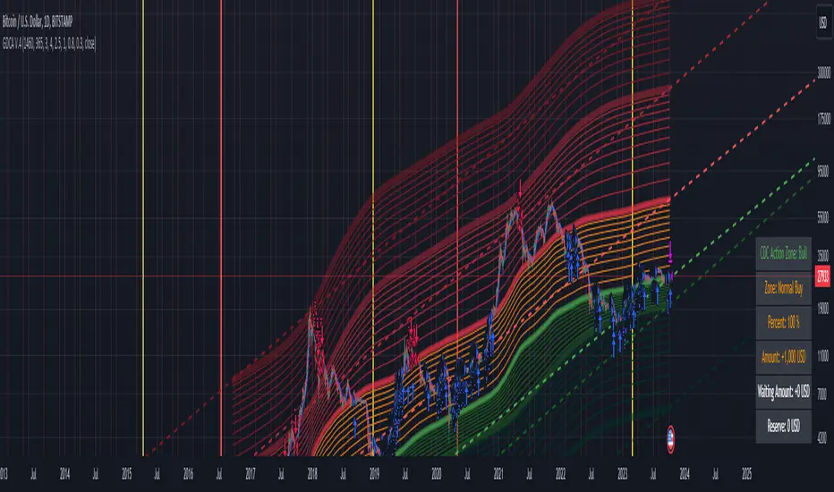
Grospector DCA V.4This is system for DCA with strategy and can trade on trend technique "CDC Action Zone".
We upgrade Grospector DCA V.3 by minimizing unnecessary components and it is not error price predictions.
This has 5 zone Extreme high , high , normal , low , Extreme low. You can dynamic set min - max percent every zone.
Extreme zone is derivative short and long which It change Extreme zone to Normal zone all position will be closed.
Every Zone is splitted 10 channel. and this strategy calculate contribution.
and now can predict price in future.
Idea : Everything has average in its life. For bitcoin use 4 years for halving. I think it will be interesting price.
Default : I set MA is 365*4 days and average it again with 365 days.
Input :
len: This input represents the length of the moving average.
strongLen: This input represents the length of the moving average used to calculate the strong buy and strong sell zone.
shortMulti: This input represents the multiplier * moveing average used to calculate the short zone.
strongSellMulti: This input represents the multiplier used to calculate the strong sell signal.
sellMulti: This input represents the multiplier * moveing average used to calculate the sell zone.
strongBuyMulti: This input represents the multiplier used to calculate the strong sell signal.
longMulti: This input represents the multiplier * moveing average used to calculate the long zone.
*Diff sellMulti and strongBuyMulti which is normal zone.
useDerivative: This input is a boolean flag that determines whether to use the derivative display zone. If set to true, the derivative display zone will be used, otherwise it will be hidden.
zoneSwitch: This input determines where to display the channel signals. A value of 1 will display the signals in all zones, a value of 2 will display the signals in the chart pane, a value of 3 will display the signals in the data window, and a value of 4 will hide the signals.
price: Defines the price source used for the indicator calculations. The user can select from various options, with the default being the closing price.
labelSwitch: Defines whether to display assistive text on the chart. The user can select a boolean value (true/false), with the default being true.
zoneSwitch: Defines which areas of the chart to display assistive zones. The user can select from four options: 1 = all, 2 = chart only, 3 = data only, 4 = none. The default value is 2.
predictFuturePrice: Defines whether to display predicted future prices on the chart. The user can select a boolean value (true/false), with the default being true.
DCA: Defines the dollar amount to use for dollar-cost averaging (DCA) trades. The user can input an integer value, with a default value of 5.
WaitingDCA: Defines the amount of time to wait before executing a DCA trade. The user can input a float value, with a default value of 0.
Invested: Defines the amount of money invested in the asset. The user can input an integer value, with a default value of 0.
strategySwitch: Defines whether to turn on the trading strategy. The user can select a boolean value (true/false), with the default being true.
seperateDayOfMonth: Defines a specific day of the month on which to execute trades. The user can input an integer value from 1-31, with the default being 28.
useReserve: Defines whether to use a reserve amount for trading. The user can select a boolean value (true/false), with the default being true.
useDerivative: Defines whether to use derivative data for the indicator calculations. The user can select a boolean value (true/false), with the default being true.
useHalving: Defines whether to use halving data for the indicator calculations. The user can select a boolean value (true/false), with the default being true.
extendHalfOfHalving: Defines the amount of time to extend the halving date. The user can input an integer value, with the default being 200.
Every Zone: It calculate percent from top to bottom which every zone will be splited 10 step.
To effectively make the DCA plan, I recommend adopting a comprehensive strategy that takes into consideration your mindset as the best indicator of the optimal approach. By leveraging your mindset, the task can be made more manageable and adaptable to any market
Dollar-cost averaging (DCA) is a suitable investment strategy for sound money and growth assets which It is Bitcoin, as it allows for consistent and disciplined investment over time, minimizing the impact of market volatility and potential risks associated with market timing
SMC StrategyThis Pine Script strategy is based on Smart Money Concepts (SMC), designed for TradingView. Here's a brief summary of what the script does:
1. Swing High and Low Calculation: It identifies recent swing highs and lows, which are used to define key zones.
2. Equilibrium, Premium, and Discount Zones:
- Equilibrium is the midpoint between the swing high and low.
- Premium Zone is above the equilibrium, indicating a potential resistance area (sell zone).
- Discount Zone is below the equilibrium, indicating a potential support area (buy zone).
3. Simple Moving Average (SMA): It uses a 50-period SMA to determine the trend direction. If the price is above the SMA, the trend is bullish; if it's below, the trend is bearish.
4. Buy and Sell Signals:
- Buy Signal: Generated when the price is in the discount zone and above the equilibrium, with the price also above the SMA.
- Sell Signal: Triggered when the price is in the premium zone and below the equilibrium, with the price also below the SMA.
5. Order Blocks: It detects basic order blocks by identifying the highest high and lowest low within the last 20 bars. These levels help confirm the buy and sell signals.
6. Liquidity Zones: It marks the swing high and low as potential liquidity zones, indicating where price may reverse due to institutional players' activity.
The strategy then executes trades based on these signals, plotting buy and sell markers on the chart and showing the key levels (zones) and trend direction.

Random Coin Toss Strategy📌 Overview
This strategy is a probability-based trading simulation that randomly decides trade direction using a coin-toss mechanism and executes trades with a customizable risk-reward ratio. It's designed primarily for testing entry frequency and risk dynamics, not predictive accuracy.
🎯 Core Concept
Every N bars (configurable), the strategy performs a pseudo-random coin toss.
Based on the result:
If heads → Buy
If tails → Sell
Once a position is opened, it sets a Stop-Loss (SL) and Take-Profit (TP) based on a multiple of the current ATR (Average True Range) value.
⚙️ Configurable Inputs
ATR Length Period for ATR calculation, determines volatility basis.
SL Multiplier SL distance = ATR × multiplier (e.g., 1.0 means 1x ATR) .
TP Multiplier TP distance = ATR × multiplier (e.g., 2.0 = 2x ATR) .
Entry Frequency Bars to wait between each new coin toss decision.
Show TP/SL Zones Toggle on/off for drawing visual TP and SL zones.
Box Size Number of bars used to define the width of the TP/SL boxes.
🔁 Entry & Exit Logic
Entry:
Happens only when no current position exists and it's the correct bar interval.
Entry direction is randomly decided.
Exit:
Positions exit at either:
Take-Profit (TP) level
Stop-Loss (SL) level
Both are calculated using the configured ATR-based distances.
🖼️ Visual Features
TP and SL zones:
Rendered as shaded rectangles (boxes) only once per trade.
Green box for TP zone, red box for SL zone.
Automatically deleted and redrawn for each new trade to avoid chart clutter.
ATR Display Table:
A minimal info table at the top-right shows the current ATR value.
Updates every few bars for performance.
🧪 Use Cases
Ideal for risk-reward modeling, strategy prototyping, and understanding how volatility-based SL/TP behavior affects results.
Great for backtesting frequency, RR tweaks (e.g., 2:5 or 3:1), and execution structure in random conditions.
⚠️ Disclaimer
Since the trade direction is random, this script is not meant for predictive trading but serves as a powerful experiment framework for studying how SL, TP, and volatility interact with random chance in a controlled, repeatable system.

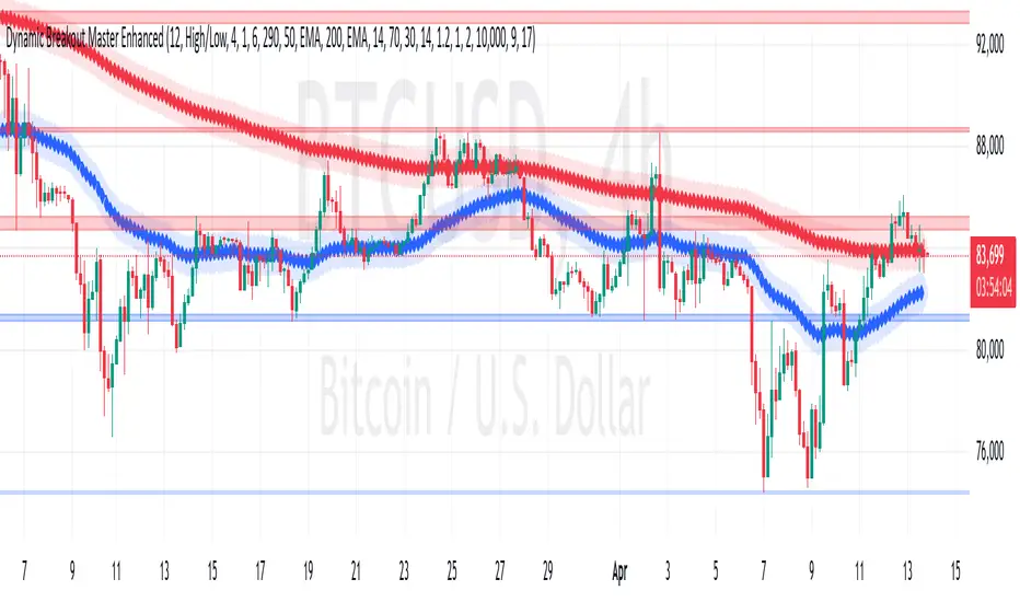
Dynamic Breakout Master by tradingbauhaus 🌟 Code Description:
This Pine Script implements a trading strategy called "Dynamic Breakout Master" 💥. The core idea of the strategy is to identify breakouts (price movements) at key support 💙 and resistance 🔴 levels, through a dynamic channel that adapts to the market’s conditions. Here's how it works:
🔧 Customizable Input Parameters:
🧭 Pivot Period: This defines the number of bars (candles) to the left and right used to detect pivots (highs and lows) that mark the support and resistance zones.
📊 Data Source: You can choose whether to use highs and lows or closes and opens of the candles to identify the pivots.
📏 Max Channel Width: Specifies the maximum width allowed for the support/resistance channel, expressed as a percentage over the last 300 bars.
💪 Minimum Pivot Strength: This defines the minimum number of pivots needed for a support or resistance level to be considered valid.
🏔 Max Support/Resistance Zones: Limits the number of key zones displayed on the chart.
📅 Lookback Period: Adjusts how many bars back the system should check to find and validate support and resistance levels.
🎨 Custom Colors: You can choose colors for the support, resistance, and in-channel zones.
📉 Moving Averages (MA): The strategy allows adding up to two moving averages (SMA or EMA) to assist in making trading decisions.
📊 Calculating Support/Resistance Levels:
The system uses an algorithm to identify pivots from prices and calculates dynamic support and resistance zones 🔒🔓.
The closer the pivots are and the stronger their influence, the more relevant the zone becomes for the strategy.
The dynamic channel is drawn on the chart, with a maximum width limit for these zones defined by the input parameter.
📈 Trading Logic:
🚀 Identifying Breakouts:
The strategy looks for when the price breaks (breakouts) a resistance or support level.
If the price breaks upward through the resistance level, a buy order 📈 is triggered.
If the price breaks downward through the support level, a sell order 📉 is triggered.
🔔 Alerts:
Resistance Break (ResBreak) and Support Break (SupBreak) alerts are configured to notify users when a significant breakout occurs.
💰 Commissions:
The strategy includes a commission (0.1%) to simulate transaction costs for each trade.
📊 Chart Visualization:
The support and resistance zones are displayed as colored rectangles:
🔴 Resistance (red) and
🔵 Support (blue).
Pivots of support and resistance can be labeled as P (for resistance) and V (for support).
Breakouts of support or resistance levels are marked with triangles that appear on the chart 🔺🔻.
📈 Trading Strategy:
If the price breaks upward through the resistance level, a long position (buy) 📈 is opened.
If the price breaks downward through the support level, a short position (sell) 📉 is opened.
🏆 Conclusion:
This script is a dynamic breakout strategy 💥 that allows traders to capture significant price movements when support or resistance channels break. The customizable parameters let users fine-tune the strategy according to their preferences, while the visual alerts on the chart make it easier to follow trading opportunities. The inclusion of moving averages and key price zones adds an extra layer of analysis to improve decision-making 💡.
EMA bands + leledc + bollinger bands trend following strategy v2The basics:
In its simplest form, this strategy is a positional trend following strategy which enters long when price breaks out above "middle" EMA bands and closes or flips short when price breaks down below "middle" EMA bands. The top and bottom of the middle EMA bands are calculated from the EMA of candle highs and lows, respectively.
The idea is that entering trades on breakouts of the high EMAs and low EMAs rather than the typical EMA based on candle closes gives a bit more confirmation of trend strength and minimizes getting chopped up. To further reduce getting chopped up, the strategy defaults to close on crossing the opposite EMA band (ie. long on break above high EMA middle band and close below low EMA middle band).
This strategy works on all markets on all timeframes, but as a trend following strategy it works best on markets prone to trending such as crypto and tech stocks. On lower timeframes, longer EMAs tend to work best (I've found good results on EMA lengths even has high up to 1000), while 4H charts and above tend to work better with EMA lengths 21 and below.
As an added filter to confirm the trend, a second EMA can be used. Inputting a slower EMA filter can ensure trades are entered in accordance with longer term trends, inputting a faster EMA filter can act as confirmation of breakout strength.
Bar coloring can be enabled to quickly visually identify a trend's direction for confluence with other indicators or strategies.
The goods:
Waiting for the trend to flip before closing a trade (especially when a longer base EMA is used) often leaves money on the table. This script combines a number of ways to identify when a trend is exhausted for backtesting the best early exits.
"Delayed bars inside middle bands" - When a number of candle's in a row open and close between the middle EMA bands, it could be a sign the trend is weak, or that the breakout was not the start of a new trend. Selecting this will close out positions after a number of bars has passed
"Leledc bars" - Originally introduced by glaz, this is a price action indicator that highlights a candle after a number of bars in a row close the same direction and result in greatest high/low over a period. It often triggers when a strong trend has paused before further continuation, or it marks the end of a trend. To mitigate closing on false Leledc signals, this strategy has two options: 1. Introducing requirement for increased volume on the Leledc bars can help filter out Leledc signals that happen mid trend. 2. Closing after a number of Leledc bars appear after position opens. These two options work great in isolation but don't perform well together in my testing.
"Bollinger Bands exhaustion bars" - These bars are highlighted when price closes back inside the Bollinger Bands and RSI is within specified overbought/sold zones. The idea is that a trend is overextended when price trades beyond the Bollinger Bands. When price closes back inside the bands it's likely due for mean reversion back to the base EMA in which this strategy will ideally re-enter a position. Since the added RSI requirements often make this indicator too strict to trigger a large enough sample size to backtest, I've found it best to use "non-standard" settings for both the bands and the RSI as seen in the default settings.
"Buy/Sell zones" - Similar to the idea behind using Bollinger Bands exhaustion bars as a closing signal. Instead of calculating off of standard deviations, the Buy/Sell zones are calculated off multiples of the middle EMA bands. When trading beyond these zones and subsequently failing back inside, price may be due for mean reversion back to the base EMA. No RSI filter is used for Buy/Sell zones.
If any early close conditions are selected, it's often worth enabling trade re-entry on "middle EMA band bounce". Instead of waiting for a candle to close back inside the middle EMA bands, this feature will re-enter position on only a wick back into the middle bands as will sometimes happen when the trend is strong.
Any and all of the early close conditions can be combined. Experimenting with these, I've found can result in less net profit but higher win-rates and sharpe ratios as less time is spent in trades.
The deadly:
The trend is your friend. But wouldn't it be nice to catch the trends early? In ranging markets (or when using slower base EMAs in this strategy), waiting for confirmation of a breakout of the EMA bands at best will cause you to miss half the move, at worst will result in getting consistently chopped up. Enabling "counter-trend" trades on this strategy will allow the strategy to enter positions on the opposite side of the EMA bands on either a Leledc bar or Bollinger Bands exhaustion bar. There is a filter requiring either a high/low (for Leledc) or open (for BB bars) outside the selected inner or outer Buy/Sell zone. There are also a number of different close conditions for the counter-trend trades to experiment with and backtest.
There are two ways I've found best to use counter-trend trades
1. Mean reverting scalp trades when a trend is clearly overextended. Selecting from the first 5 counter-trend closing conditions on the dropdown list will usually close the trades out quickly, with less profit but less risk.
2. Trying to catch trends early. Selecting any of the close conditions below the first 5 can cause the strategy to behave as if it's entering into a new trend (from the wrong side).
This feature can be deadly effective in profiting from every move price makes, or deadly to the strategy's PnL if not set correctly. Since counter-trend trades open opposite the middle bands, a stop-loss is recommended to reduce risk. If stop-losses for counter-trend trades are disabled, the strategy will hold a position open often until liquidation in a trending market if th trade is offsides. Note that using a slower base EMA makes counter-trend stop-losses even more necessary as it can reduce the effectiveness of the Buy/Sell zone filter for opening the trades as price can spend a long time trending outside the zones. If faster EMAs (34 and below) are used with "Inner" Buy/Zone filter selected, the first few closing conditions will often trigger almost immediately closing the trade at a loss.
The niche:
I've added a feature to default into longs or shorts. Enabling these with other features (aside from the basic long/short on EMA middle band breakout) tends to break the strategy one way or another. Enabling default long works to simulate trying to acquire more of the asset rather than the base currency. Enabling default short can have positive results for those high FDV, high inflation coins that go down-only for months at a time. Otherwise, I use default short as a hedge for coins that I hold and stake spot. I gain the utility and APR of staking while reducing the risk of holding the underlying asset by maintaining a net neutral position *most* of the time.
Disclaimer:
This script is intended for experimenting and backtesting different strategies around EMA bands. Use this script for your live trading at your own risk. I am a rookie coder, as such there may be errors in the code that cause the strategy to behave not as intended. As far as I can tell it doesn't repaint, but I cannot guarantee that it does not. That being said if there's any question, improvements, or errors you've found, drop a comment below!
Grospector DCA V.3This is system for DCA with strategy.
This has 5 zone Extreme high , high , normal , low , Extreme low. You can dynamic set min - max percent every zone.
Extreme zone is derivative short and long which It change Extreme zone to Normal zone all position will be closed.
Every Zone is splitted 10 channel. and this strategy calculate contribution.
and now can predict price in future.
Idea : Everything has average in its life. For bitcoin use 4 years for halving. I think it will be interesting price.
Default : I set MA is 365*4 days and average it again with 365 days.
Input :
len: This input represents the length of the moving average.
strongLen: This input represents the length of the moving average used to calculate the strong buy and strong sell zone.
shortMulti: This input represents the multiplier * moveing average used to calculate the short zone.
strongSellMulti: This input represents the multiplier used to calculate the strong sell signal.
sellMulti: This input represents the multiplier * moveing average used to calculate the sell zone.
strongBuyMulti: This input represents the multiplier used to calculate the strong sell signal.
longMulti: This input represents the multiplier * moveing average used to calculate the long zone.
*Diff sellMulti and strongBuyMulti which is normal zone.
useDerivative: This input is a boolean flag that determines whether to use the derivative display zone. If set to true, the derivative display zone will be used, otherwise it will be hidden.
zoneSwitch: This input determines where to display the channel signals. A value of 1 will display the signals in all zones, a value of 2 will display the signals in the chart pane, a value of 3 will display the signals in the data window, and a value of 4 will hide the signals.
price: Defines the price source used for the indicator calculations. The user can select from various options, with the default being the closing price.
labelSwitch: Defines whether to display assistive text on the chart. The user can select a boolean value (true/false), with the default being true.
zoneSwitch: Defines which areas of the chart to display assistive zones. The user can select from four options: 1 = all, 2 = chart only, 3 = data only, 4 = none. The default value is 2.
predictFuturePrice: Defines whether to display predicted future prices on the chart. The user can select a boolean value (true/false), with the default being true.
DCA: Defines the dollar amount to use for dollar-cost averaging (DCA) trades. The user can input an integer value, with a default value of 5.
WaitingDCA: Defines the amount of time to wait before executing a DCA trade. The user can input a float value, with a default value of 0.
Invested: Defines the amount of money invested in the asset. The user can input an integer value, with a default value of 0.
strategySwitch: Defines whether to turn on the trading strategy. The user can select a boolean value (true/false), with the default being true.
seperateDayOfMonth: Defines a specific day of the month on which to execute trades. The user can input an integer value from 1-31, with the default being 28.
useReserve: Defines whether to use a reserve amount for trading. The user can select a boolean value (true/false), with the default being true.
useDerivative: Defines whether to use derivative data for the indicator calculations. The user can select a boolean value (true/false), with the default being true.
useHalving: Defines whether to use halving data for the indicator calculations. The user can select a boolean value (true/false), with the default being true.
extendHalfOfHalving: Defines the amount of time to extend the halving date. The user can input an integer value, with the default being 200.
Every Zone : It calculate percent from top to bottom which every zone will be splited 10 step.
To effectively make the DCA plan, I recommend adopting a comprehensive strategy that takes into consideration your mindset as the best indicator of the optimal approach. By leveraging your mindset, the task can be made more manageable and adaptable to any market
Dollar-cost averaging (DCA) is a suitable investment strategy for sound money and growth assets which It is Bitcoin, as it allows for consistent and disciplined investment over time, minimizing the impact of market volatility and potential risks associated with market timing

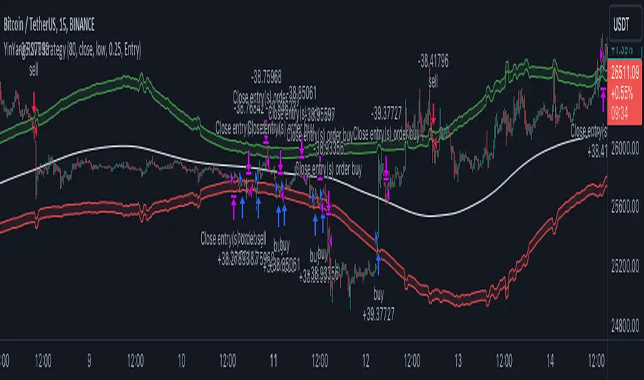
YinYang RSI Volume Trend StrategyThere are many strategies that use RSI or Volume but very few that take advantage of how useful and important the two of them combined are. This strategy uses the Highs and Lows with Volume and RSI weighted calculations on top of them. You may be wondering how much of an impact Volume and RSI can have on the prices; the answer is a lot and we will discuss those with plenty of examples below, but first…
How does this strategy work?
It’s simple really, when the purchase source crosses above the inner low band (red) it creates a Buy or Long. This long has a Trailing Stop Loss band (the outer low band that's also red) that can be adjusted in the Settings. The Stop Loss is based on a % of the inner low band’s price and by default it is 0.1% lower than the inner band’s price. This Stop Loss is not only a stop loss but it can also act as a Purchase Available location.
You can get back into a trade after a stop loss / take profit has been hit when your Reset Purchase Availability After condition has been met. This can either be at Stop Loss, Entry or None.
It is advised to allow it to reset in case the stop loss was a fake out but the call was right. Sometimes it may trigger stop loss multiple times in a row, but you don’t lose much on stop loss and you gain lots when the call is right.
The Take Profit location is the basis line (white). Take Profit occurs when the Exit Source (close, open, high, low or other) crosses the basis line and then on a different bar the Exit Source crosses back over the basis line. For example, if it was a Long and the bar’s Exit Source closed above the basis line, and then 2 bars later its Exit Source closed below the basis line, Take Profit would occur. You can disable Take Profit in Settings, but it is very useful as many times the price will cross the Basis and then correct back rather than making it all the way to the opposing zone.
Longs:
If for instance your Long doesn’t need to Take Profit and instead reaches the top zone, it will close the position when it crosses above the inner top line (green).
Please note you can change the Exit Source too which is what source (close, open, high, low) it uses to end the trades.
The Shorts work the same way as the Long but just opposite, they start when the purchase source crosses under the inner upper band (green).
Shorts:
Shorts take profit when it crosses under the basis line and then crosses back.
Shorts will Stop loss when their outer upper band (green) is crossed with the Exit Source.
Short trades are completed and closed when its Exit Source crosses under the inner low red band.
So, now that you understand how the strategy works, let’s discuss why this strategy works and how it is profitable.
First we will discuss Volume as we deem it plays a much bigger role overall and in our strategy:
As I’m sure many of you know, Volume plays a huge factor in how much something moves, but it also plays a role in the strength of the movement. For instance, let’s look at two scenarios:
Bitcoin’s price goes up $1000 in 1 Day but the Volume was only 10 million
Bitcoin’s price goes up $200 in 1 Day but the Volume was 40 million
If you were to only look at the price, you’d say #1 was more important because the price moved x5 the amount as #2, but once you factor in the volume, you know this is not true. The reason why Volume plays such a huge role in Price movement is because it shows there is a large Limit Order battle going on. It means that both Bears and Bulls believe that price is a good time to Buy and Sell. This creates a strong Support and Resistance price point in this location. If we look at scenario #2, when there is high volume, especially if it is drastically larger than the average volume Bitcoin was displaying recently, what can we decipher from this? Well, the biggest take away is that the Bull’s won the battle, and that likely when that happens we will see bullish movement continuing to happen as most of the Bears Limit Orders have been fulfilled. Whereas with #2, when large price movement happens and Bitcoin goes up $1000 with low volume what can we deduce? The main takeaway is that Bull’s pressured the price up with Market Orders where they purchased the best available price, also what this means is there were very few people who were wanting to sell. This generally dictates that Whale Limit orders for Sells/Shorts are much higher up and theres room for movement, but it also means there is likely a whale that is ready to dump and crash it back down.
You may be wondering, what did this example have to do with YinYang RSI Volume Trend Strategy? Well the reason we’ve discussed this is because we use Volume multiple times to apply multiplications in our calculations to add large weight to the price when there is lots of volume (this is applied both positively and negatively). For instance, if the price drops a little and there is high volume, our strategy will move its bounds MUCH lower than the price actually dropped, and if there was low volume but the price dropped A LOT, our strategy will only move its bounds a little. We believe this reflects higher levels of price accuracy than just price alone based on the examples described above.
Don’t believe us?
Here is with Volume NOT factored in (VWMA = SMA and we remove our Volume Filter calculation):
Which produced -$2880 Profit
Here is with our Volume factored in:
Which produced $553,000 (55.3%)
As you can see, we wen’t from $-2800 profit with volume not factored to $553,000 with volume factored. That's quite a big difference! (Please note previous success does not predict future success we are simply displaying the $ amounts as example).
Now how about RSI and why does it matter in this strategy?
As I’m sure most of you are aware, RSI is one of the leading indicators used in trading. For this reason we figured it would only make sense to incorporate it into our calculations. We fiddled with RSI for quite awhile and sometimes what logically seems to be the right way to use it isn’t. Now, because of this, our RSI calculation is a little odd, but basically what we’re doing is we calculate the RSI, then turn it into a percentage (between 0-1) that can easily be multiplied to the price point we need. The price point we use is the difference between our high purchase zone and our low purchase zone. This allows us to see how much price movement there is between zones. We multiply our zone size with our RSI multiplication and we get the amount we will add +/- to our basis line (white line). This officially creates the NEW high and low purchase zones that we are actually using and displaying in our trades.
If you found that confusing, here are some examples to why it is an important calculation for this strategy:
Before RSI factored in:
Which produced 27.8% Profit
After RSI factored in:
Which produced 553% Profit
As you can see, the RSI makes not only the purchase zones more accurate, but it also greatly increases the profit the strategy is able to make. It also helps ensure an relatively linear profit slope so you know it is reliable with its trades.
This strategy can work on pretty much anything, but you should tweak the values a bit for each pair you are trading it with for best results.
We hope you can find some use out of this simple but effective strategy, if you have any questions, comments or concerns please let us know.
HAPPY TRADING!
Crude Oil Time + Fix Catalyst StrategyHybrid Workflow: Event-Driven Macro + Market DNA Micro
1. Macro Catalyst Layer (Your Overlays)
Event Mapping: Fed decisions, LBMA fixes, EIA releases, OPEC+ meetings.
Regime Filters: Risk-on/off, volatility regimes, macro bias (hawkish/dovish).
Volatility Scaling: ATR-based position sizing, adaptive overlays for London/NY sessions.
Governance: Max trades/day, cool-down logic, session boundaries.
👉 This layer answers when and why to engage.
2. Micro Execution Layer (Market DNA)
Order Flow Confirmation: Tape reading (Level II, time & sales, bid/ask).
Liquidity Zones: Identify support/resistance pools where buyers/sellers cluster.
Imbalance Detection: Aggressive buyers/sellers overwhelming the other side.
Precision Entry: Only trigger trades when order flow confirms macro catalyst bias.
Risk Discipline: Tight stops beyond liquidity zones, conviction-based scaling.
👉 This layer answers how and where to engage.
3. Unified Playbook
Step Macro Overlay (Your Edge) Market DNA (Jay’s Edge) Result
Event Trigger Fed/LBMA/OPEC+ catalyst flagged — Volatility window opens
Bias Filter Hawkish/dovish regime filter — Directional bias set
Sizing ATR volatility scaling — Position size calibrated
Execution — Tape confirms liquidity imbalance Precision entry
Risk Control Governance rules (cool-down, max trades) Tight stops beyond liquidity zones Disciplined exits
4. Gold & Silver Use Case
Gold (Fed Day):
Overlay flags volatility window → bias hawkish.
Market DNA shows sellers hitting bids at resistance.
Enter short with volatility-scaled size, stop just above liquidity zone.
Silver (LBMA Fix):
Overlay highlights fix window → bias neutral.
Market DNA shows buyers stepping in at support.
Enter long with adaptive size, HUD displays risk metrics.
5. HUD Integration
Macro Dashboard: Catalyst timeline, regime filter status, volatility bands.
Micro Dashboard: Live tape imbalance meter, liquidity zone map, conviction score.
Unified View: Macro tells you when to look, micro tells you when to pull the trigger.
⚡ This hybrid workflow gives you macro awareness + micro precision. Your overlays act as the radar, Jay’s Market DNA acts as the laser scope. Together, they create a disciplined, event-aware, volatility-scaled playbook for gold and silver.
Antonio — do you want me to draft this into a compile-safe Pine Script v6 template that embeds the macro overlay logic, while leaving hooks for Market DNA-style execution (order flow confirmation)? That way you’d have a production-ready skeleton to extend across TradingView, TradeStation, and NinjaTrader.
Antonio — do you want me to draft this into a compile-safe Pine Script v6 template that embeds the macro overlay logic, while leaving hooks for Market DNA-style execution (order flow confirmation)? That way you’d have a production-ready skeleton to extend across TradingView, TradeStation, and NinjaTrader.

BOCS Channel Scalper Strategy - Automated Mean Reversion System# BOCS Channel Scalper Strategy - Automated Mean Reversion System
## WHAT THIS STRATEGY DOES:
This is an automated mean reversion trading strategy that identifies consolidation channels through volatility analysis and executes scalp trades when price enters entry zones near channel boundaries. Unlike breakout strategies, this system assumes price will revert to the channel mean, taking profits as price bounces back from extremes. Position sizing is fully customizable with three methods: fixed contracts, percentage of equity, or fixed dollar amount. Stop losses are placed just outside channel boundaries with take profits calculated either as fixed points or as a percentage of channel range.
## KEY DIFFERENCE FROM ORIGINAL BOCS:
**This strategy is designed for traders seeking higher trade frequency.** The original BOCS indicator trades breakouts OUTSIDE channels, waiting for price to escape consolidation before entering. This scalper version trades mean reversion INSIDE channels, entering when price reaches channel extremes and betting on a bounce back to center. The result is significantly more trading opportunities:
- **Original BOCS**: 1-3 signals per channel (only on breakout)
- **Scalper Version**: 5-15+ signals per channel (every touch of entry zones)
- **Trade Style**: Mean reversion vs trend following
- **Hold Time**: Seconds to minutes vs minutes to hours
- **Best Markets**: Ranging/choppy conditions vs trending breakouts
This makes the scalper ideal for active day traders who want continuous opportunities within consolidation zones rather than waiting for breakout confirmation. However, increased trade frequency also means higher commission costs and requires tighter risk management.
## TECHNICAL METHODOLOGY:
### Price Normalization Process:
The strategy normalizes price data to create consistent volatility measurements across different instruments and price levels. It calculates the highest high and lowest low over a user-defined lookback period (default 100 bars). Current close price is normalized using: (close - lowest_low) / (highest_high - lowest_low), producing values between 0 and 1 for standardized volatility analysis.
### Volatility Detection:
A 14-period standard deviation is applied to the normalized price series to measure price deviation from the mean. Higher standard deviation values indicate volatility expansion; lower values indicate consolidation. The strategy uses ta.highestbars() and ta.lowestbars() to identify when volatility peaks and troughs occur over the detection period (default 14 bars).
### Channel Formation Logic:
When volatility crosses from a high level to a low level (ta.crossover(upper, lower)), a consolidation phase begins. The strategy tracks the highest and lowest prices during this period, which become the channel boundaries. Minimum duration of 10+ bars is required to filter out brief volatility spikes. Channels are rendered as box objects with defined upper and lower boundaries, with colored zones indicating entry areas.
### Entry Signal Generation:
The strategy uses immediate touch-based entry logic. Entry zones are defined as a percentage from channel edges (default 20%):
- **Long Entry Zone**: Bottom 20% of channel (bottomBound + channelRange × 0.2)
- **Short Entry Zone**: Top 20% of channel (topBound - channelRange × 0.2)
Long signals trigger when candle low touches or enters the long entry zone. Short signals trigger when candle high touches or enters the short entry zone. This captures mean reversion opportunities as price reaches channel extremes.
### Cooldown Filter:
An optional cooldown period (measured in bars) prevents signal spam by enforcing minimum spacing between consecutive signals. If cooldown is set to 3 bars, no new long signal will fire until 3 bars after the previous long signal. Long and short cooldowns are tracked independently, allowing both directions to signal within the same period.
### ATR Volatility Filter:
The strategy includes a multi-timeframe ATR filter to avoid trading during low-volatility conditions. Using request.security(), it fetches ATR values from a specified timeframe (e.g., 1-minute ATR while trading on 5-minute charts). The filter compares current ATR to a user-defined minimum threshold:
- If ATR ≥ threshold: Trading enabled
- If ATR < threshold: No signals fire
This prevents entries during dead zones where mean reversion is unreliable due to insufficient price movement.
### Take Profit Calculation:
Two TP methods are available:
**Fixed Points Mode**:
- Long TP = Entry + (TP_Ticks × syminfo.mintick)
- Short TP = Entry - (TP_Ticks × syminfo.mintick)
**Channel Percentage Mode**:
- Long TP = Entry + (ChannelRange × TP_Percent)
- Short TP = Entry - (ChannelRange × TP_Percent)
Default 50% targets the channel midline, a natural mean reversion target. Larger percentages aim for opposite channel edge.
### Stop Loss Placement:
Stop losses are placed just outside the channel boundary by a user-defined tick offset:
- Long SL = ChannelBottom - (SL_Offset_Ticks × syminfo.mintick)
- Short SL = ChannelTop + (SL_Offset_Ticks × syminfo.mintick)
This logic assumes channel breaks invalidate the mean reversion thesis. If price breaks through, the range is no longer valid and position exits.
### Trade Execution Logic:
When entry conditions are met (price in zone, cooldown satisfied, ATR filter passed, no existing position):
1. Calculate entry price at zone boundary
2. Calculate TP and SL based on selected method
3. Execute strategy.entry() with calculated position size
4. Place strategy.exit() with TP limit and SL stop orders
5. Update info table with active trade details
The strategy enforces one position at a time by checking strategy.position_size == 0 before entry.
### Channel Breakout Management:
Channels are removed when price closes more than 10 ticks outside boundaries. This tolerance prevents premature channel deletion from minor breaks or wicks, allowing the mean reversion setup to persist through small boundary violations.
### Position Sizing System:
Three methods calculate position size:
**Fixed Contracts**:
- Uses exact contract quantity specified in settings
- Best for futures traders (e.g., "trade 2 NQ contracts")
**Percentage of Equity**:
- position_size = (strategy.equity × equity_pct / 100) / close
- Dynamically scales with account growth
**Cash Amount**:
- position_size = cash_amount / close
- Maintains consistent dollar exposure regardless of price
## INPUT PARAMETERS:
### Position Sizing:
- **Position Size Type**: Choose Fixed Contracts, % of Equity, or Cash Amount
- **Number of Contracts**: Fixed quantity per trade (1-1000)
- **% of Equity**: Percentage of account to allocate (1-100%)
- **Cash Amount**: Dollar value per position ($100+)
### Channel Settings:
- **Nested Channels**: Allow multiple overlapping channels vs single channel
- **Normalization Length**: Lookback for high/low calculation (1-500, default 100)
- **Box Detection Length**: Period for volatility detection (1-100, default 14)
### Scalping Settings:
- **Enable Long Scalps**: Toggle long entries on/off
- **Enable Short Scalps**: Toggle short entries on/off
- **Entry Zone % from Edge**: Size of entry zone (5-50%, default 20%)
- **SL Offset (Ticks)**: Distance beyond channel for stop (1+, default 5)
- **Cooldown Period (Bars)**: Minimum spacing between signals (0 = no cooldown)
### ATR Filter:
- **Enable ATR Filter**: Toggle volatility filter on/off
- **ATR Timeframe**: Source timeframe for ATR (1, 5, 15, 60 min, etc.)
- **ATR Length**: Smoothing period (1-100, default 14)
- **Min ATR Value**: Threshold for trade enablement (0.1+, default 10.0)
### Take Profit Settings:
- **TP Method**: Choose Fixed Points or % of Channel
- **TP Fixed (Ticks)**: Static distance in ticks (1+, default 30)
- **TP % of Channel**: Dynamic target as channel percentage (10-100%, default 50%)
### Appearance:
- **Show Entry Zones**: Toggle zone labels on channels
- **Show Info Table**: Display real-time strategy status
- **Table Position**: Corner placement (Top Left/Right, Bottom Left/Right)
- **Color Settings**: Customize long/short/TP/SL colors
## VISUAL INDICATORS:
- **Channel boxes** with semi-transparent fill showing consolidation zones
- **Colored entry zones** labeled "LONG ZONE ▲" and "SHORT ZONE ▼"
- **Entry signal arrows** below/above bars marking long/short entries
- **Active TP/SL lines** with emoji labels (⊕ Entry, 🎯 TP, 🛑 SL)
- **Info table** showing position status, channel state, last signal, entry/TP/SL prices, and ATR status
## HOW TO USE:
### For 1-3 Minute Scalping (NQ/ES):
- ATR Timeframe: "1" (1-minute)
- ATR Min Value: 10.0 (for NQ), adjust per instrument
- Entry Zone %: 20-25%
- TP Method: Fixed Points, 20-40 ticks
- SL Offset: 5-10 ticks
- Cooldown: 2-3 bars
- Position Size: 1-2 contracts
### For 5-15 Minute Day Trading:
- ATR Timeframe: "5" or match chart
- ATR Min Value: Adjust to instrument (test 8-15 for NQ)
- Entry Zone %: 20-30%
- TP Method: % of Channel, 40-60%
- SL Offset: 5-10 ticks
- Cooldown: 3-5 bars
- Position Size: Fixed contracts or 5-10% equity
### For 30-60 Minute Swing Scalping:
- ATR Timeframe: "15" or "30"
- ATR Min Value: Lower threshold for broader market
- Entry Zone %: 25-35%
- TP Method: % of Channel, 50-70%
- SL Offset: 10-15 ticks
- Cooldown: 5+ bars or disable
- Position Size: % of equity recommended
## BACKTEST CONSIDERATIONS:
- Strategy performs best in ranging, mean-reverting markets
- Strong trending markets produce more stop losses as price breaks channels
- ATR filter significantly reduces trade count but improves quality during low volatility
- Cooldown period trades signal quantity for signal quality
- Commission and slippage materially impact sub-5-minute timeframe performance
- Shorter timeframes require tighter entry zones (15-20%) to catch quick reversions
- % of Channel TP adapts better to varying channel sizes than fixed points
- Fixed contract sizing recommended for consistent risk per trade in futures
**Backtesting Parameters Used**: This strategy was developed and tested using realistic commission and slippage values to provide accurate performance expectations. Recommended settings: Commission of $1.40 per side (typical for NQ futures through discount brokers), slippage of 2 ticks to account for execution delays on fast-moving scalp entries. These values reflect real-world trading costs that active scalpers will encounter. Backtest results without proper cost simulation will significantly overstate profitability.
## COMPATIBLE MARKETS:
Works on any instrument with price data including stock indices (NQ, ES, YM, RTY), individual stocks, forex pairs (EUR/USD, GBP/USD), cryptocurrency (BTC, ETH), and commodities. Volume-based features require data feed with volume information but are optional for core functionality.
## KNOWN LIMITATIONS:
- Immediate touch entry can fire multiple times in choppy zones without adequate cooldown
- Channel deletion at 10-tick breaks may be too aggressive or lenient depending on instrument tick size
- ATR filter from lower timeframes requires higher-tier TradingView subscription (request.security limitation)
- Mean reversion logic fails in strong breakout scenarios leading to stop loss hits
- Position sizing via % of equity or cash amount calculates based on close price, may differ from actual fill price
- No partial closing capability - full position exits at TP or SL only
- Strategy does not account for gap openings or overnight holds
## RISK DISCLOSURE:
Trading involves substantial risk of loss. Past performance does not guarantee future results. This strategy is for educational purposes and backtesting only. Mean reversion strategies can experience extended drawdowns during trending markets. Stop losses may not fill at intended levels during extreme volatility or gaps. Thoroughly test on historical data and paper trade before risking real capital. Use appropriate position sizing and never risk more than you can afford to lose. Consider consulting a licensed financial advisor before making trading decisions. Automated trading systems can malfunction - monitor all live positions actively.
## ACKNOWLEDGMENT & CREDITS:
This strategy is built upon the channel detection methodology created by **AlgoAlpha** in the "Smart Money Breakout Channels" indicator. Full credit and appreciation to AlgoAlpha for pioneering the normalized volatility approach to identifying consolidation patterns. The core channel formation logic using normalized price standard deviation is AlgoAlpha's original contribution to the TradingView community.
Enhancements to the original concept include: mean reversion entry logic (vs breakout), immediate touch-based signals, multi-timeframe ATR volatility filtering, flexible position sizing (fixed/percentage/cash), cooldown period filtering, dual TP methods (fixed points vs channel percentage), automated strategy execution with exit management, and real-time position monitoring table.

IU EMA Channel StrategyIU EMA Channel Strategy
Overview:
The IU EMA Channel Strategy is a simple yet effective trend-following strategy that uses two Exponential Moving Averages (EMAs) based on the high and low prices. It provides clear entry and exit signals by identifying price crossovers relative to the EMAs while incorporating a built-in Risk-to-Reward Ratio (RTR) for effective risk management.
Inputs ( Settings ):
- RTR (Risk-to-Reward Ratio): Define the ratio for risk-to-reward (default = 2).
- EMA Length: Adjust the length of the EMA channels (default = 100).
How the Strategy Works
1. EMA Channels:
- High-based EMA: EMA calculated on the high price.
- Low-based EMA: EMA calculated on the low price.
The area between these two EMAs creates a "channel" that visually highlights potential support and resistance zones.
2. Entry Rules:
- Long Entry: When the price closes above the high-based EMA (crossover).
- Short Entry: When the price closes below the low-based EMA (crossunder).
These entries ensure trades are taken in the direction of momentum.
3. Stop Loss (SL) and Take Profit (TP):
- Stop Loss:
- For long positions, the SL is set at the previous bar's low.
- For short positions, the SL is set at the previous bar's high.
- Take Profit:
- TP is automatically calculated using the Risk-to-Reward Ratio (RTR) you define.
- Example: If RTR = 2, the TP will be 2x the risk distance.
4. Exit Rules:
- Positions are closed at either the stop loss or the take profit level.
- The strategy manages exits automatically to enforce disciplined risk management.
Visual Features
1. EMA Channels:
- The high and low EMAs are dynamically color-coded:
- Green: Price is above the EMA (bullish condition).
- Red: Price is below the EMA (bearish condition).
- The area between the EMAs is shaded for better visual clarity.
2. Stop Loss and Take Profit Zones:
- SL and TP levels are plotted for both long and short positions.
- Zones are filled with:
- Red: Stop Loss area.
- Green: Take Profit area.
Be sure to manage your risk and position size properly.

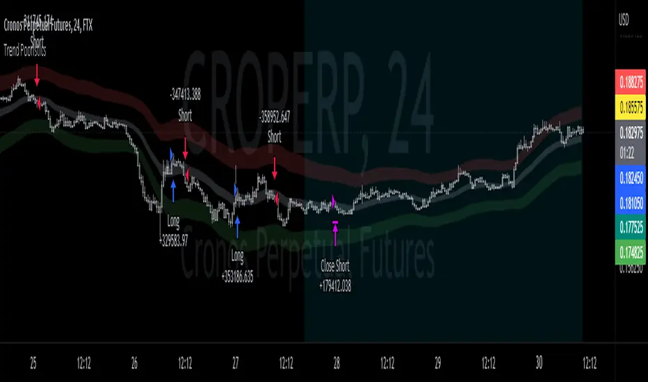
Trend Pullback System```{"variant":"standard","id":"36492","title":"Trend Pullback System Description"}
Trend Pullback System is a price-action trend continuation model that looks to enter on pullbacks, not breakouts. It’s designed to find high-quality long/short entries inside an already established trend, place the stop at meaningful structure, trail that stop as structure evolves, and warn you when the trade thesis is no longer valid.
Developed by: Mohammed Bedaiwi
---------------------------------
HOW IT WORKS
---------------------------------
1. Trend Detection
• The strategy defines overall bias using moving averages.
• Bullish environment (“uptrend”): price above the slower MA, fast MA above slow MA, and the slow MA is sloping up.
• Bearish environment (“downtrend”): price below the slower MA, fast MA below slow MA, and the slow MA is sloping down.
This prevents trading against chop and focuses on continuation moves in the dominant direction.
2. Pullback + Re-entry Logic
• The script waits for price to pull back into structure (support in an uptrend, resistance in a downtrend), and then push back in the direction of the main trend.
• That “push back” is the setup trigger. We don’t chase the first breakout candle — we buy/sell the retest + resume.
3. Structural Levels (“Diamonds”)
• Green diamond (below bar): bullish pivot low formed while the trend is bullish. This marks defended support.
- Use it as a re-entry zone for longs.
- Use it to trail a stop higher when you’re already long.
- Shorts can take profit here because buyers stepped in.
• Red diamond (above bar): bearish pivot high formed while the trend is bearish. This marks defended resistance.
- Use it as a re-entry zone for shorts.
- Use it to trail a stop lower when you’re already short.
- Longs can take profit here because sellers stepped in.
4. Entry Signals
• BUY arrow (green triangle up under the candle, text like “BUY” / “BUY Zone”):
- LongSetup is true.
- Trend is bullish or turning bullish.
- Price just bounced off recent defended support (green diamond) and reclaimed short-term momentum.
Meaning: enter long here or cover/exit shorts.
• SELL arrow (red triangle down above the candle):
- ShortSetup is true.
- Trend is bearish or turning bearish.
- Price just rolled down from defended resistance (red diamond) and lost short-term momentum.
Meaning: enter short here or take profit on longs.
These are the primary trade entries. They are meant to be actionable.
5. Weak Setups (“W” in yellow)
• Yellow triangle with “W”:
- A possible long/short idea is trying to form, BUT the higher-timeframe confirmation is not fully there yet.
- Think of it as early pressure / early caution, not a full signal.
• You usually watch these areas rather than jumping in immediately.
6. Exit Warning (orange “EXIT” label above a bar)
• The strategy will raise an EXIT marker when you’re in a trade and the *opposite* side just produced a confirmed setup.
- You’re short and a valid longSetup appears → EXIT.
- You’re long and a valid shortSetup appears → EXIT.
• This is basically: “Close or reduce — the other side just took control.”
• It’s not just a trailing stop hit; it’s a regime flip warning.
7. Stop, Target, and Trailing
• On every new setup, the script records:
- Initial stop: recent swing beyond the defended level (below support for longs, above resistance for shorts).
- Initial target: recent opposing swing.
• While you’re in position, if new confirming diamonds print in your favor, the stop can trail toward the new defended level.
• This creates structure-based risk management (not just fixed % or ATR).
8. Reference Levels
• The strategy also plots prior higher-timeframe closes (last week’s close, last month’s close, last year’s close). These can behave as magnets or stall points.
• They’re helpful for take-profit timing and for reading “are we trading above or below last month’s close?”
9. Momentum Panel (hidden by default)
• Internally, the script calculates an SMI-style momentum oscillator with overbought/oversold zones.
• This is optional visual confirmation and does not drive the core entry/exit logic.
---------------------------------
WHAT A TRADE LOOKS LIKE IN REAL PRICE ACTION
---------------------------------
Early warning
• Yellow W + red diamonds + red down arrows = “This is getting weak. Short setups are here.”
• You may also see something like “My Short Entry Id.” That’s where the short side actually engages.
Bearish follow-through, then exhaustion
• Price bleeds down.
• Then the orange EXIT appears.
→ Translation: “If you’re still short, close it. Buyers are stepping in hard. Risk of reversal is now high.”
Regime flip
• Right after EXIT, multiple green BUY arrows fire together (“BUY”, “BUYZone”).
• That’s the true long trigger.
→ This is where you either enter long or flip from short to long.
Expansion leg
• After that flip, price rips up for multiple candles / days / weeks.
• While it runs:
- Green diamonds appear under pullbacks → “dip buy zones / trail stop up here.”
- More BUY arrows show on minor pullbacks → continuation long / scale adds.
Distribution / topping
• Later, you start seeing new yellow W triangles again near local highs. That’s your “careful, this might be topping” warning.
• You finally get a hard red candle, and green diamonds stop stacking.
→ That’s where you tighten risk, scale out, or assume the move is mature.
In plain terms, the model is doing the following for you:
• It puts you short during weakness.
• It tells you when to get OUT of the short.
• It flips you long right as control changes.
• It gives you a structure-based trail the whole way up.
• It warns you again when momentum at the top starts cracking.
That is exactly how the logic was designed.
---------------------------------
QUICK INTERPRETATION CHEAT SHEET
---------------------------------
🔻 Red triangle + “Short Entry” near a red diamond
→ Short entry zone (or take profit on a long).
🟥 Red diamond above bar
→ Sellers defended here. Treat it as resistance. Good place to trail short stops just above that level. Avoid chasing longs straight into it.
🟨 Yellow W
→ Attention only. Early pressure / possible turn. Not fully confirmed.
🟧 EXIT (orange label)
→ The opposite side just printed a real setup. Close the old idea (cover shorts if you’re short, exit longs if you’re long). Thesis invalid.
🟩 Burst of green BUY triangles after EXIT
→ Long entry. Also a “cover shorts now” alert. This is the core money entry in bullish reversals.
💎 Green diamond below bar
→ Bulls defended that level. Good for trailing your long stop up, and good “buy the dip in trend” locations.
📈 Blue / teal MAs stacked and rising
→ Confirmed bullish structure. You’re in trend continuation mode, so dips are opportunities, not automatic exits.
---------------------------------
COLOR / SHAPE KEY
---------------------------------
• Green triangle up (“BUY”, “BUY Zone”):
Long entry / cover shorts / continuation long trigger.
• Red triangle down:
Short entry / take profit on longs / continuation short trigger.
• Orange “EXIT” label:
Opposite side just fired a real setup. The previous trade thesis is now invalid.
• Green diamond below price:
Bullish defended support in an uptrend. Use for dip buys, trailing stops on longs, and objective cover zones for shorts.
• Red diamond above price:
Bearish defended resistance in a downtrend. Use for re-entry shorts, trailing stops on shorts, and objective scale-out zones for longs.
• Yellow “W”:
Weak / early potential setup. Watch it, don’t blindly trust it.
• Moving average bands (fast MA, slow MA, Hull MA):
When stacked and rising, bullish control. When stacked and falling, bearish control.
---------------------------------
INTENT
---------------------------------
This system is built to:
• Trade with momentum, not against it.
• Enter on pullbacks into proven structure, not chase stretched breakouts.
• Automate stop/target logic around actual defended swing levels.
• Warn you when the other side takes over so you don’t give back gains.
Typical usage:
1. In an uptrend, wait for price to pull back, print a green diamond (support proved), then take the first BUY arrow that fires.
2. In a downtrend, wait for a bounce into resistance, print a red diamond (sellers proved), then take the first SELL arrow that fires.
3. Respect EXIT when it appears — that’s the model saying “this trade is done.”
---------------------------------
DISCLAIMER
---------------------------------
This script is for educational and research purposes only. It is not financial advice, investment advice, or a recommendation to buy or sell any security, cryptoasset, or derivative. Markets carry risk. Past performance does not guarantee future results. You are fully responsible for your own decisions, position sizing, risk management, and compliance with all applicable laws and regulations.

RSI Divergence StrategyOverview
The RSI Divergence Strategy Indicator is a trading tool that uses the RSI and divergences created to generate high-probability buy and sell signals.
I have provided the best formula of numbers to use for BTC on a 30 minute timeframe.
You can change where on RSI you enter and exit both long or short trades. This way you can experiment on different tokens using different entry/exit points. Can use on multiple timeframes.
This strategy is designed to open and close long or short trades based on the levels you provide it. You can then check on the RSI where the best levels are for each token you want to trade and amend it as required to generate a profitable strategy.
How It Works
The RSI Divergence Strategy Indicator uses bear and bull divergences in conjuction with a level you have input on the RSI.
RSI for Overbought/Oversold:
• Input variables for entry and exit levels and when the entry levels combine with a bear or bull divergence signal, a trade is alerted.
RSI Divergence:
• Buy and sell signals are confirmed when the RSI creates bearish or bullish divergences and these divergences are in the same area as your levels you input for entry to short or long.
After 7 years of experience and testing I have calculated the exact numbers required and produced a formula to calculate the exact input variables for a 30 minute Bitcoin chart.
Key Features
1️⃣ Divergence Identification – Ensures trades are taken only when a bull or bear divergence has formed.
2️⃣ Overbought/Oversold Input Filtering – Set up your own variables on the RSI for different markets after identifying patterns on the RSI in relation to a bearish or bullish divergence.
3️⃣ Works on any chart – Suitable for all markets and timeframes once you input the correct variables for entry and exit levels.
How to Use
🟢 Basic Trading:
• Use on any timeframe.
• Enter trade only when alert has fired off. Close when it says to exit.
• Change entry and exit levels in the properties of the strategy indicator.
• Make entry and exit levels coincide with bearish or bullish divergences on the RSI.
Check the strategy tester to see backtesting so you know if the indicator is profitable or not for that market and timeframe as each crypto token is different and so is the timeframe you choose.
📢 Webhook Automation:
• Set up TradingView Alerts to auto-execute trades via Webhook-compatible platforms.
Key additions for divergence visualization:
Divergence Arrows:
Bullish divergence: Green label with white 'bull ' text
Bearish divergence: Red label with white 'bear' text
Positioned at the pivot point
Divergence Lines:
Connects consecutive RSI pivot points
Automatically drawn between consecutive pivot points
Enhanced RSI Coloring:
Overbought zone: Red
Oversold zone: Green
Neutral zone: Gray
The visualization helps you instantly spot:
Where divergences are forming on the RSI
The pattern of higher lows (bullish) or lower highs (bearish)
Contextual coloring of RSI relative to standard levels
All divergence markers appear at the correct historical pivot points, making it easy to visually confirm divergence patterns as they develop.
Strategy levels and background zones also shown to help visual look.
Why This Combination?
This indicator is just a simple RSI tool.
It is designed to filter out weak trades and only execute trades that have:
✅ RSI Divergence
✅ Overbought or Oversold Conditions
It does not calculate downtrends or bear markets so care is recommended taking long trades during these times.
Why It’s Worth Using?
📈 Open Source – Free to use and learn from.
📉 Long or Short Term Trading Style – Entry/Exit parameters options are designed for both short or long term trades allowing you to experiment until you find a profitable strategy for that market you want to trade.
📢 Seamless Webhook Automation – Execute trades automatically with TradingView alerts.
💲 Ready to trade smarter?
✅ Add the RSI Divergence Strategy Indicator to your TradingView chart.
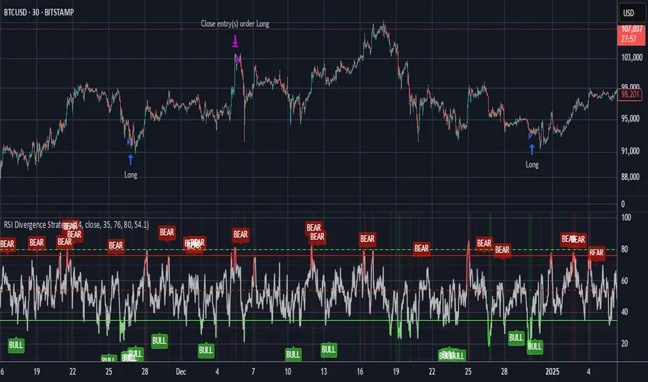
ALT Risk Metric StrategyHere's a professional write-up for your ALT Risk Strategy script:
ALT/BTC Risk Strategy - Multi-Crypto DCA with Bitcoin Correlation Analysis
Overview
This strategy uses Bitcoin correlation as a risk indicator to time entries and exits for altcoins. By analyzing how your chosen altcoin performs relative to Bitcoin, the strategy identifies optimal accumulation periods (when alt/BTC is oversold) and profit-taking opportunities (when alt/BTC is overbought). Perfect for traders who want to outperform Bitcoin by strategically timing altcoin positions.
Key Innovation: Why Alt/BTC Matters
Most traders focus solely on USD price, but Alt/BTC ratios reveal true altcoin strength:
When Alt/BTC is low → Altcoin is undervalued relative to Bitcoin (buy opportunity)
When Alt/BTC is high → Altcoin has outperformed Bitcoin (take profits)
This approach captures the rotation between BTC and alts that drives crypto cycles
Key Features
📊 Advanced Technical Analysis
RSI (60% weight): Primary momentum indicator on weekly timeframe
Long-term MA Deviation (35% weight): Measures distance from 150-period baseline
MACD (5% weight): Minor confirmation signal
EMA Smoothing: Filters noise while maintaining responsiveness
All calculations performed on Alt/BTC pairs for superior market timing
💰 3-Tier DCA System
Level 1 (Risk ≤ 70): Conservative entry, base allocation
Level 2 (Risk ≤ 50): Increased allocation, strong opportunity
Level 3 (Risk ≤ 30): Maximum allocation, extreme undervaluation
Continuous buying: Executes every bar while below threshold for true DCA behavior
Cumulative sizing: L3 triggers = L1 + L2 + L3 amounts combined
📈 Smart Profit Management
Sequential selling: Must complete L1 before L2, L2 before L3
Percentage-based exits: Sell portions of position, not fixed amounts
Auto-reset on re-entry: New buy signals reset sell progression
Prevents premature full exits during volatile conditions
🤖 3Commas Automation
Pre-configured JSON webhooks for Custom Signal Bots
Multi-exchange support: Binance, Coinbase, Kraken, Bitfinex, Bybit
Flexible quote currency: USD, USDT, or BUSD
Dynamic order sizing: Automatically adjusts to your tier thresholds
Full webhook documentation compliance
🎨 Multi-Asset Support
Pre-configured for popular altcoins:
ETH (Ethereum)
SOL (Solana)
ADA (Cardano)
LINK (Chainlink)
UNI (Uniswap)
XRP (Ripple)
DOGE
RENDER
Custom option for any other crypto
How It Works
Risk Metric Calculation (0-100 scale):
Fetches weekly Alt/BTC price data for stability
Calculates RSI, MACD, and deviation from 150-period MA
Normalizes MACD to 0-100 range using 500-bar lookback
Combines weighted components: (MACD × 0.05) + (RSI × 0.60) + (Deviation × 0.35)
Applies 5-period EMA smoothing for cleaner signals
Color-Coded Risk Zones:
Green (0-30): Extreme buying opportunity - Alt heavily oversold vs BTC
Lime/Yellow (30-70): Accumulation range - favorable risk/reward
Orange (70-85): Caution zone - consider taking initial profits
Red/Maroon (85-100+): Euphoria zone - aggressive profit-taking
Entry Logic:
Buys execute every candle when risk is below threshold
As risk decreases, position sizing automatically scales up
Example: If risk drops from 60→25, you'll be buying at L1 rate until it hits 50, then L2 rate, then L3 rate
Exit Logic:
Sells only trigger when in profit AND risk exceeds thresholds
Sequential execution ensures partial profit-taking
If new buy signal occurs before all sells complete, sell levels reset to L1
Configuration Guide
Choosing Your Altcoin:
Select crypto from dropdown (or use CUSTOM for unlisted coins)
Pick your exchange
Choose quote currency (USD, USDT, BUSD)
Risk Metric Tuning:
Long Term MA (default 150): Higher = more extreme signals, Lower = more frequent
RSI Length (default 10): Lower = more volatile, Higher = smoother
Smoothing (default 5): Increase for less noise, decrease for faster reaction
Buy Settings (Aggressive DCA Example):
L1 Threshold: 70 | Amount: $5
L2 Threshold: 50 | Amount: $6
L3 Threshold: 30 | Amount: $7
Total L3 buy = $18 per candle when deeply oversold
Sell Settings (Balanced Exit Example):
L1: 70 threshold, 25% position
L2: 85 threshold, 35% position
L3: 100 threshold, 40% position (final exit)
3Commas Setup
Bot Configuration:
Create Custom Signal Bot in 3Commas
Set trading pair to your altcoin/USD (e.g., ETH/USD, SOL/USDT)
Order size: Select "Send in webhook, quote" to use strategy's dollar amounts
Copy Bot UUID and Secret Token
Script Configuration:
Paste credentials into 3Commas section inputs
Check "Enable 3Commas Alerts"
Save and apply to chart
TradingView Alert:
Create Alert → Condition: "alert() function calls only"
Webhook URL: api.3commas.io
Enable "Webhook URL" checkbox
Expiration: Open-ended
Strategy Advantages
✅ Outperform Bitcoin: Designed specifically to beat BTC by timing alt rotations
✅ Capture Alt Seasons: Automatically accumulates when alts lag, sells when they pump
✅ Risk-Adjusted Sizing: Buys more when cheaper (better risk/reward)
✅ Emotional Discipline: Systematic approach removes fear and FOMO
✅ Multi-Asset: Run same strategy across multiple altcoins simultaneously
✅ Proven Indicators: Combines RSI, MACD, and MA deviation - battle-tested tools
Backtesting Insights
Optimal Timeframes:
Daily chart: Best for backtesting and signal generation
Weekly data is fetched internally regardless of display timeframe
Historical Performance Characteristics:
Accumulates heavily during bear markets and BTC dominance periods
Captures explosive altcoin rallies when BTC stagnates
Sequential selling preserves capital during extended downtrends
Works best on established altcoins with multi-year history
Risk Considerations:
Requires capital reserves for extended accumulation periods
Some altcoins may never recover if fundamentals deteriorate
Past correlation patterns may not predict future performance
Always size positions according to personal risk tolerance
Visual Interface
Indicator Panel Displays:
Dynamic color line: Green→Lime→Yellow→Orange→Red as risk increases
Horizontal threshold lines: Dashed lines mark your buy/sell levels
Entry/Exit labels: Green labels for buys, Orange/Red/Maroon for sells
Real-time risk value: Numerical display on price scale
Customization:
All threshold lines are adjustable via inputs
Color scheme clearly differentiates buy zones (green spectrum) from sell zones (red spectrum)
Line weights emphasize most extreme thresholds (L3 buy and L3 sell)
Strategy Philosophy
This strategy is built on the principle that altcoins move in cycles relative to Bitcoin. During Bitcoin rallies, alts often bleed against BTC (high sell, accumulate). When Bitcoin consolidates, alts pump (take profits). By measuring risk on the Alt/BTC chart instead of USD price, we time these rotations with precision.
The 3-tier system ensures you're always averaging in at better prices and scaling out at better prices, maximizing your Bitcoin-denominated returns.
Advanced Tips
Multi-Bot Strategy:
Run this on 5-10 different altcoins simultaneously to:
Diversify correlation risk
Capture whichever alt is pumping
Smooth equity curve through rotation
Pairing with BTC Strategy:
Use alongside the BTC DCA Risk Strategy for complete portfolio coverage:
BTC strategy for core holdings
ALT strategies for alpha generation
Rebalance between them based on BTC dominance
Threshold Calibration:
Check 2-3 years of historical data for your chosen alt
Note where risk metric sat during major bottoms (set buy thresholds)
Note where it peaked during euphoria (set sell thresholds)
Adjust for your risk tolerance and holding period
Credits
Strategy Development & 3Commas Integration: Claude AI (Anthropic)
Technical Analysis Framework: RSI, MACD, Moving Average theory
Implementation: pommesUNDwurst
Disclaimer
This strategy is for educational purposes only. Cryptocurrency trading involves substantial risk of loss. Altcoins are especially volatile and many fail completely. The strategy assumes liquid markets and reliable Alt/BTC price data. Always do your own research, understand the fundamentals of any asset you trade, and never risk more than you can afford to lose. Past performance does not guarantee future results. The authors are not financial advisors and assume no liability for trading decisions.
Additional Warning: Using leverage or trading illiquid altcoins amplifies risk significantly. This strategy is designed for spot trading of established cryptocurrencies with deep liquidity.
Tags: Altcoin, Alt/BTC, DCA, Risk Metric, Dollar Cost Averaging, 3Commas, ETH, SOL, Crypto Rotation, Bitcoin Correlation, Automated Trading, Alt Season
Feel free to modify any sections to better match your style or add specific backtesting results you've observed! 🚀Claude is AI and can make mistakes. Please double-check responses. Sonnet 4.5

🧪 Yuri Garcia Smart Money Strategy FULL (Slope Divergence))📣 Yuri Garcia – Smart Money Strategy FULL
This is my private Smart Money Concept strategy, designed for my family and community to learn, trade, and grow sustainably.
🔑 How it works:
✅ Volume Cluster Zones: Automatically detects areas where strong buyers or sellers concentrate, acting as dynamic S/R levels.
✅ HTF Institutional Zones (4H): Higher timeframe trend filter ensures you’re always trading in the direction of major flows.
✅ Wick Pullback Filter: Confirms price rejects the zone, catching smart money traps and reversals.
✅ Cumulative Delta (CVD): Confirms whether buyers or sellers are truly in control.
✅ Slope-Based Divergence: Optional hidden divergence between price & CVD to spot reversals others miss.
✅ ATR Dynamic SL/TP: Adapts stop loss and take profit to live volatility with adjustable risk/reward.
🧩 Visual Markers Explained:
🟦 Blue X: Price inside HTF zone
🟨 Yellow X: Price inside Volume Cluster zone
🟧 Orange Circle: Wick pullback detected
🟥 Red Square: CVD confirms order flow strength
🔼 Aqua Triangle Up: Bullish slope divergence
🔽 Purple Triangle Down: Bearish slope divergence
🟢 Green Triangle Up: Final Long Entry confirmed
🔴 Red Triangle Down: Final Short Entry confirmed
⚡ Who is this for?
This strategy is best suited for traders who understand smart money concepts, order flow, and want an adaptive framework to trade major assets like BTC, Gold, SP500, NASDAQ, or FX pairs.
🔒 Important
Use responsibly, backtest extensively, and combine with solid risk management. This is for educational purposes only.
✨ Credits
Built with ❤️ by Yuri Garcia – dedicated to my family & community.
✅ How to use it
1️⃣ Add to chart
2️⃣ Adjust inputs for your asset & timeframe
3️⃣ Enable/disable slope divergence filter to match your style
4️⃣ Set your alerts with built-in conditions
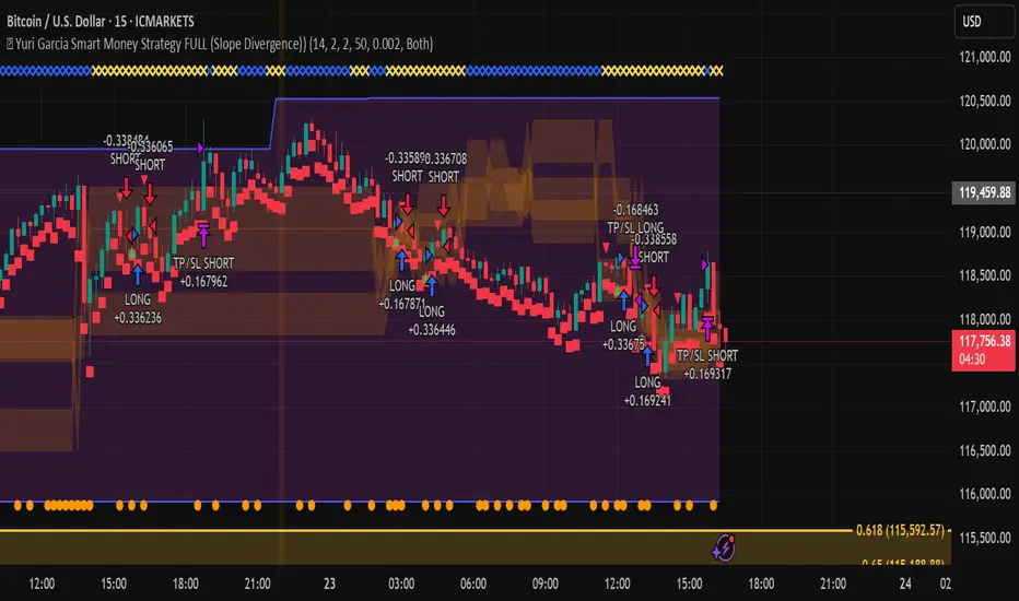
PowerZone Trading StrategyExplanation of the PowerZone Trading Strategy for Your Users
The PowerZone Trading Strategy is an automated trading strategy that detects strong price movements (called "PowerZones") and generates signals to enter a long (buy) or short (sell) position, complete with predefined take profit and stop loss levels. Here’s how it works, step by step:
1. What is a PowerZone?
A "PowerZone" (PZ) is a zone on the chart where the price has shown a significant and consistent movement over a specific number of candles (bars). There are two types:
Bullish PowerZone (Bullish PZ): Occurs when the price rises consistently over several candles after an initial bearish candle.
Bearish PowerZone (Bearish PZ): Occurs when the price falls consistently over several candles after an initial bullish candle.
The code analyzes:
A set number of candles (e.g., 5, adjustable via "Periods").
A minimum percentage move (adjustable via "Min % Move for PowerZone") to qualify as a strong zone.
Whether to use the full candle range (highs and lows) or just open/close prices (toggle with "Use Full Range ").
2. How Does It Detect PowerZones?
Bullish PowerZone:
Looks for an initial bearish candle (close below open).
Checks that the next candles (e.g., 5) are all bullish (close above open).
Ensures the total price movement exceeds the minimum percentage set.
Defines a range: from the high (or open) to the low of the initial candle.
Bearish PowerZone:
Looks for an initial bullish candle (close above open).
Checks that the next candles are all bearish (close below open).
Ensures the total price movement exceeds the minimum percentage.
Defines a range: from the high to the low (or close) of the initial candle.
These zones are drawn on the chart with lines: green or white for bullish, red or blue for bearish, depending on the color scheme ("DARK" or "BRIGHT").
3. When Does It Enter a Trade?
The strategy waits for a breakout from the PowerZone range to enter a trade:
Buy (Long): When the price breaks above the high of a Bullish PowerZone.
Sell (Short): When the price breaks below the low of a Bearish PowerZone.
The position size is set to 100% of available equity (adjustable in the code).
4. Take Profit and Stop Loss
Take Profit (TP): Calculated as a multiple (adjustable via "Take Profit Factor," default 1.5) of the PowerZone height. For example:
For a buy, TP = Entry price + (PZ height × 1.5).
For a sell, TP = Entry price - (PZ height × 1.5).
Stop Loss (SL): Calculated as a multiple (adjustable via "Stop Loss Factor," default 1.0) of the PZ height, placed below the range for buys or above for sells.
5. Visualization on the Chart
PowerZones are displayed with lines on the chart (you can hide them with "Show Bullish Channel" or "Show Bearish Channel").
An optional info panel ("Show Info Panel") displays key levels: PZ high and low, TP, and SL.
You can also enable brief documentation on the chart ("Show Documentation") explaining the basic rules.
6. Alerts
The code generates automatic alerts in TradingView:
For a bullish breakout: "Bullish PowerZone Breakout - LONG!"
For a bearish breakdown: "Bearish PowerZone Breakdown - SHORT!"
7. Customization
You can tweak:
The number of candles to detect a PZ ("Periods").
The minimum percentage move ("Min % Move").
Whether to use highs/lows or just open/close ("Use Full Range").
The TP and SL factors.
The color scheme and what elements to display on the chart.
Practical Example
Imagine you set "Periods = 5" and "Min % Move = 2%":
An initial bearish candle appears, followed by 5 consecutive bullish candles.
The total move exceeds 2%.
A Bullish PowerZone is drawn with a high and low.
If the price breaks above the high, you enter a long position with a TP 1.5 times the PZ height and an SL equal to the height below.
The system executes the trade and exits automatically at TP or SL.
Conclusion
This strategy is great for capturing strong price movements after consolidation or momentum zones. It’s automated, visual, and customizable, making it useful for both beginner and advanced traders. Try it out and adjust it to fit your trading style!
Rally Base Drop SND Pivots Strategy [LuxAlgo X PineIndicators]This strategy is based on the Rally Base Drop (RBD) SND Pivots indicator developed by LuxAlgo. Full credit for the concept and original indicator goes to LuxAlgo.
The Rally Base Drop SND Pivots Strategy is a non-repainting supply and demand trading system that detects pivot points based on Rally, Base, and Drop (RBD) candles. This strategy automatically identifies key market structure levels, allowing traders to:
Identify pivot-based supply and demand (SND) zones.
Use fixed criteria for trend continuation or reversals.
Filter out market noise by requiring structured price formations.
Enter trades based on breakouts of key SND pivot levels.
How the Rally Base Drop SND Pivots Strategy Works
1. Pivot Point Detection Using RBD Candles
The strategy follows a rigid market structure methodology, where pivots are detected only when:
A Rally (R) consists of multiple consecutive bullish candles.
A Drop (D) consists of multiple consecutive bearish candles.
A Base (B) is identified as a transition between Rallies and Drops, acting as a pivot point.
The pivot level is confirmed when the formation is complete.
Unlike traditional fractal-based pivots, RBD Pivots enforce stricter structural rules, ensuring that each pivot:
Has a well-defined bullish or bearish price movement.
Reduces false signals caused by single-bar fluctuations.
Provides clear supply and demand levels based on structured price movements.
These pivot levels are drawn on the chart using color-coded boxes:
Green zones represent bullish pivot levels (Rally Base formations).
Red zones represent bearish pivot levels (Drop Base formations).
Once a pivot is confirmed, the high or low of the base candle is used as the reference level for future trades.
2. Trade Entry Conditions
The strategy allows traders to select from three trading modes:
Long Only – Only takes long trades when bullish pivot breakouts occur.
Short Only – Only takes short trades when bearish pivot breakouts occur.
Long & Short – Trades in both directions based on pivot breakouts.
Trade entry signals are triggered when price breaks through a confirmed pivot level:
Long Entry:
A bullish pivot level is formed.
Price breaks above the bullish pivot level.
The strategy enters a long position.
Short Entry:
A bearish pivot level is formed.
Price breaks below the bearish pivot level.
The strategy enters a short position.
The strategy includes an optional mode to reverse long and short conditions, allowing traders to experiment with contrarian entries.
3. Exit Conditions Using ATR-Based Risk Management
This strategy uses the Average True Range (ATR) to calculate dynamic stop-loss and take-profit levels:
Stop-Loss (SL): Placed 1 ATR below entry for long trades and 1 ATR above entry for short trades.
Take-Profit (TP): Set using a Risk-Reward Ratio (RR) multiplier (default = 6x ATR).
When a trade is opened:
The entry price is recorded.
ATR is calculated at the time of entry to determine stop-loss and take-profit levels.
Trades exit automatically when either SL or TP is reached.
If reverse conditions mode is enabled, stop-loss and take-profit placements are flipped.
Visualization & Dynamic Support/Resistance Levels
1. Pivot Boxes for Market Structure
Each pivot is marked with a colored box:
Green boxes indicate bullish demand zones.
Red boxes indicate bearish supply zones.
These boxes remain on the chart to act as dynamic support and resistance levels, helping traders identify key price reaction zones.
2. Horizontal Entry, Stop-Loss, and Take-Profit Lines
When a trade is active, the strategy plots:
White line → Entry price.
Red line → Stop-loss level.
Green line → Take-profit level.
Labels display the exact entry, SL, and TP values, updating dynamically as price moves.
Customization Options
This strategy offers multiple adjustable settings to optimize performance for different market conditions:
Trade Mode Selection → Choose between Long Only, Short Only, or Long & Short.
Pivot Length → Defines the number of required Rally & Drop candles for a pivot.
ATR Exit Multiplier → Adjusts stop-loss distance based on ATR.
Risk-Reward Ratio (RR) → Modifies take-profit level relative to risk.
Historical Lookback → Limits how far back pivot zones are displayed.
Color Settings → Customize pivot box colors for bullish and bearish setups.
Considerations & Limitations
Pivot Breakouts Do Not Guarantee Reversals. Some pivot breaks may lead to continuation moves instead of trend reversals.
Not Optimized for Low Volatility Conditions. This strategy works best in trending markets with strong momentum.
ATR-Based Stop-Loss & Take-Profit May Require Optimization. Different assets may require different ATR multipliers and RR settings.
Market Noise May Still Influence Pivots. While this method filters some noise, fake breakouts can still occur.
Conclusion
The Rally Base Drop SND Pivots Strategy is a non-repainting supply and demand system that combines:
Pivot-based market structure analysis (using Rally, Base, and Drop candles).
Breakout-based trade entries at confirmed SND levels.
ATR-based dynamic risk management for stop-loss and take-profit calculation.
This strategy helps traders:
Identify high-probability supply and demand levels.
Trade based on structured market pivots.
Use a systematic approach to price action analysis.
Automatically manage risk with ATR-based exits.
The strict pivot detection rules and built-in breakout validation make this strategy ideal for traders looking to:
Trade based on market structure.
Use defined support & resistance levels.
Reduce noise compared to traditional fractals.
Implement a structured supply & demand trading model.
This strategy is fully customizable, allowing traders to adjust parameters to fit their market and trading style.
Full credit for the original concept and indicator goes to LuxAlgo.
BTC DCA Risk Metric StrategyBTC DCA Risk Strategy - Automated Dollar Cost Averaging with 3Commas Integration
Overview
This strategy combines the proven Oakley Wood Risk Metric with an intelligent tiered Dollar Cost Averaging (DCA) system, designed to help traders systematically accumulate Bitcoin during periods of low risk and take profits during high-risk conditions.
Key Features
📊 Multi-Component Risk Assessment
4-Year SMA Deviation: Measures Bitcoin's distance from its long-term mean
20-Week MA Analysis: Tracks medium-term momentum shifts
50-Day/50-Week MA Ratio: Captures short-to-medium term trend strength
All metrics are normalized by time to account for Bitcoin's maturing market dynamics
💰 3-Tier DCA Buy System
Level 1 (Low Risk): Conservative entry with base allocation
Level 2 (Lower Risk): Increased allocation as opportunity improves
Level 3 (Extreme Low Risk): Maximum allocation during rare buying opportunities
Buys execute every bar while risk remains below thresholds, enabling true DCA accumulation
📈 Progressive Profit Taking
Sell Level 1: Take initial profits as risk increases
Sell Level 2: Scale out further positions during elevated risk
Sell Level 3: Final exit during extreme market conditions
Sell levels automatically reset when new buy signals occur, allowing flexible re-entry
🤖 3Commas Integration
Fully automated webhook alerts for Custom Signal Bots
JSON payloads formatted per 3Commas API specifications
Supports multiple exchanges (Binance, Coinbase, Kraken, Gemini, Bybit)
Configurable quote currency (USD, USDT, BUSD)
How It Works
The strategy calculates a composite risk metric (0-1 scale):
0.0-0.2: Extreme buying opportunity (green zone)
0.2-0.5: Favorable accumulation range (yellow zone)
0.5-0.8: Neutral to cautious territory (orange zone)
0.8-1.0+: High risk, profit-taking zone (red zone)
Buy Logic: As risk decreases, position sizes increase automatically. If risk drops from L1 to L3 threshold, the strategy combines all three tier allocations for maximum exposure.
Sell Logic: Sequential profit-taking ensures you capture gains progressively. The system won't advance to Sell L2 until L1 completes, preventing premature full exits.
Configuration
Risk Metric Parameters:
All calculations use Bitcoin price data (any BTC chart works)
Time-normalized formulas adapt to market maturity
No manual parameter tuning required
Buy Settings:
Set risk thresholds for each tier (default: 0.20, 0.10, 0.00)
Define dollar amounts per tier (default: $10, $15, $20)
Fully customizable to your risk tolerance and capital
Sell Settings:
Configure risk thresholds for profit-taking (default: 1.00, 1.50, 2.00)
Set percentage of position to sell at each level (default: 25%, 35%, 40%)
3Commas Setup:
Create a Custom Signal Bot in 3Commas
Copy Bot UUID and Secret Token into strategy inputs
Enable 3Commas Alerts checkbox
Create TradingView alert: Condition → "alert() function calls only", Webhook → api.3commas.io
Backtesting Results
Strengths:
Systematically buys dips without emotion
Averages down during extended bear markets
Captures explosive bull run profits through tiered exits
Pyramiding (1000 max orders) allows true DCA behavior
Considerations:
Requires sufficient capital for multiple buys during prolonged downtrends
Backtest on Daily timeframe for most reliable signals
Past performance does not guarantee future results
Visual Design
The indicator pane displays:
Color-coded risk metric line: Changes from white→red→orange→yellow→green as risk decreases
Background zones: Green (buy), yellow (hold), red (sell) areas
Dashed threshold lines: Clear visual markers for each buy/sell level
Entry/Exit labels: Green buy labels and orange/red sell labels mark all trades
Credits
Original Risk Metric: Oakley Wood
Strategy Development & 3Commas Integration: Claude AI (Anthropic)
Modifications: pommesUNDwurst
Disclaimer
This strategy is for educational and informational purposes only. Cryptocurrency trading carries substantial risk of loss. Always conduct your own research and never invest more than you can afford to lose. The authors are not financial advisors and assume no responsibility for trading decisions made using this tool.

USDJPY Fair Value Gap + Session Strategy🎯 Overview
This strategy combines Fair Value Gaps (FVGs) with session-based order flow analysis, specifically optimized for USDJPY. It identifies price inefficiencies left behind by institutional order flow during high-volatility trading sessions, offering a modern alternative to traditional lagging indicators.
🔬 What Are Fair Value Gaps?
Fair Value Gaps represent areas where aggressive institutional buying or selling created "gaps" in the market structure:
Bullish FVG: Price moves up so aggressively that it leaves unfilled buy orders behind
Bearish FVG: Price moves down so quickly that it leaves unfilled sell orders behind
Research shows approximately 80% of FVGs get "filled" (price returns to the gap) within 20-60 bars, making them highly predictable trading zones.
(see the generated image above)
(see the generated image above)
FVG Detection Logic:
text
// Bullish FVG: Gap between high and current low
bullishFVG = low > high and high > high
// Bearish FVG: Gap between low and current high
bearishFVG = high < low and low < low
🌏 Session-Based Trading
Why Sessions Matter for USDJPY
(see the generated image above)
Tokyo Session (00:00-09:00 UTC)
Highest volatility during first hour (00:00-01:00 UTC)
Average movement: 51-60 pips
Best for breakout strategies
London/NY Overlap (13:00-16:00 UTC)
Maximum liquidity and institutional participation
Tightest spreads and most reliable FVG formations
Optimal for continuation trades
Monday Premium Effect
USDJPY moves 120+ pips on Mondays due to weekend positioning
Enhanced FVG formation during session opens
📊 Strategy Components
(see the generated image above)
1. Fair Value Gap Detection
Identifies bullish and bearish FVGs automatically
Age limit: FVGs expire after 20 bars to avoid stale setups
Size filter: Minimum gap size to filter out noise
2. Session Filtering
Tokyo Open focus: Trades during first hour of Asian session
London/NY Overlap: Captures high-liquidity institutional flows
Weekend gap strategy: Enhanced signals on Monday opens
3. Volume Confirmation
Requires 1.5x average volume spike
Confirms institutional participation
Reduces false signals
4. Trend Alignment
50 EMA filter ensures trades align with higher timeframe trend
Long trades above EMA, short trades below
Prevents costly counter-trend trades
5. Risk Management
2:1 Risk/Reward minimum ensures profitability with 40%+ win rate
Percentage-based stops adapt to USDJPY volatility (0.3% default)
Configurable position sizing
🎯 Entry Conditions
(see the generated image above)
Long Entry (BUY)
✅ Bullish FVG detected in previous bars
✅ Price returns to FVG zone during active trading session
✅ Volume spike above 1.5x average
✅ Price above 50 EMA (trend confirmation)
✅ Bullish candle closes within FVG zone
✅ Trading during Tokyo open OR London/NY overlap
Short Entry (SELL)
✅ Bearish FVG detected in previous bars
✅ Price returns to FVG zone during active trading session
✅ Volume spike above 1.5x average
✅ Price below 50 EMA (trend confirmation)
✅ Bearish candle closes within FVG zone
✅ Trading during Tokyo open OR London/NY overlap
📈 Expected Performance
Backtesting Results (Based on Similar Strategies):
Win Rate: 44-59% (profitable due to high R:R ratio)
Average Winner: 60-90 pips during London/NY sessions
Average Loser: 30-40 pips (tight stops at FVG boundaries)
Risk/Reward: 2:1 minimum, often 3:1 during strong trends
Best Performance: Monday Tokyo opens and Wednesday London/NY overlaps
Why This Works for USDJPY:
90% correlation with US-Japan bond yield spreads
High volatility provides sufficient pip movement
Heavy institutional/central bank participation creates clear FVGs
Consistent volatility patterns across trading sessions
⚙️ Configurable Parameters
Session Settings:
Trade Tokyo Session (Enable/Disable)
Trade London/NY Overlap (Enable/Disable)
FVG Settings:
FVG Minimum Size (Filter small gaps)
Maximum FVG Age (20 bars default)
Show FVG Markers (Visual display)
Volume Settings:
Use Volume Filter (Enable/Disable)
Volume Multiplier (1.5x default)
Volume Average Period (20 bars)
Trend Settings:
Use Trend Filter (Enable/Disable)
Trend EMA Period (50 default)
Risk Management:
Risk/Reward Ratio (2.0 default)
Stop Loss Percentage (0.3% default)
🎨 Visual Indicators
🟡 Yellow Line: 50 EMA trend filter
🟢 Green Triangles: Long entry signals
🔴 Red Triangles: Short entry signals
🟢 Green Dots: Bullish FVG zones
🔴 Red Dots: Bearish FVG zones
🟦 Blue Background: Tokyo open session
🟧 Orange Background: London/NY overlap
📊 Recommended Settings
Optimal Timeframes:
Primary: 5-minute charts (scalping)
Secondary: 15-minute charts (swing trading)
Parameter Optimization:
Conservative: Stop Loss 0.2%, R:R 2:1, Volume 2.0x
Balanced: Stop Loss 0.3%, R:R 2:1, Volume 1.5x (default)
Aggressive: Stop Loss 0.4%, R:R 1.5:1, Volume 1.2x
Risk Management:
Maximum 1-2% of account per trade
Daily loss limit: Stop after 3-5 consecutive losses
Use fixed percentage position sizing
⚠️ Important Considerations
Avoid Trading During:
Major news events (BOJ interventions, NFP, FOMC)
Holiday periods with reduced liquidity
Low volatility Asian afternoon sessions
When US-Japan yield differential narrows sharply
Best Practices:
Limit to 2-3 trades per session maximum
Always respect the 50 EMA trend filter
Never risk more than planned per trade
Paper trade for 2-4 weeks before live implementation
Track performance by session and day of week
🚀 How to Use
Add the script to your USDJPY chart
Set timeframe to 5-minute or 15-minute
Adjust parameters based on your risk tolerance
Enable strategy alerts for automated notifications
Wait for visual signals (triangles) to appear
Enter trades according to your risk management rules
📚 Strategy Foundation
This strategy is based on:
Smart Money Concepts (SMC): Institutional order flow tracking
Market Microstructure: Understanding how FVGs form in electronic trading
Quantified Risk Management: Statistical edge through proper R:R ratios
Session Liquidity Patterns: Exploiting predictable volatility cycles