1M XAU Cumulative Delta Volume with OB Breakouts
### Overview
This is a **session-based CVD strategy** built around the **00:00–07:00 CEST range**. It finds the high/low of that session, turns them into **adaptive ATR-based support (yellow)** and **resistance (purple)** zones, and trades only **CVD-confirmed reversals** off those levels.
---
### How it Works
* For each day, the script:
* Builds a 00:00–07:00 CEST **profile high/low**.
* Creates a **support zone** around the session low and a **resistance zone** around the session high.
* Using lower timeframe data, it reconstructs **Cumulative Volume Delta (CVD)** and a **recent delta** filter.
* It arms “pending” states when price **enters a zone from the correct side**, then confirms:
* **BUY (long):** price reclaims above support and recent CVD is strongly positive.
* **SELL (short):** price rejects below resistance and recent CVD is strongly negative.
Only these two CVD signals (`buySignal` / `sellSignal`) open trades.
---
### Strategy Logic
* **Entries**
* `buySignal` → open **long** (if flat).
* `sellSignal` → open **short** (if flat).
* No pyramiding; one position at a time.
* **Exits (only TP & SL)**
* Long: TP at `avg_price * (0.5 + TP%)`, SL at `avg_price * (1 – SL%)`.
* Short: TP at `avg_price * (0.5 – TP%)`, SL at `avg_price * (1 + SL%)`.
* No opposite-signal exits.
---
### Extras
* **Reversal markers** on yellow/purple zones and **breakout/retest markers** are plotted for context and alerts but **do not trigger entries**.
* Zone width and “thickening” are ATR-based so important touches and near-touches are easy to see.
* Only suited for **1m intraday scalping** (e.g. XAU/USD), but can be tested on other markets/timeframes.
Cari dalam skrip untuk "zone"

Volume weighted average price band strategy [Kevin-Patrick]VWAP Bands strategy, Credit
VWAP Machine Learning Bands is an advanced indicator designed to enhance trading analysis by integrating VWAP with a machine learning-inspired adaptive smoothing approach. This tool helps traders identify trend-based support and resistance zones, predict potential price movements, and generate dynamic trade signals.
Key Features
Adaptive ML VWAP Calculation: Uses a dynamically adjusted SMA-based VWAP model with volatility sensitivity for improved trend analysis.
Forecasting Mechanism: The 'Forecast' parameter shifts the ML output forward, providing predictive insights into potential price movements.
Volatility-Based Band Adjustments: The 'Sigma' parameter fine-tunes the impact of volatility on ML smoothing, adapting to market conditions.
Multi-Tier Standard Deviation Bands: Includes two levels of bands to define potential breakout or mean-reversion zones.
Dynamic Trend-Based Colouring: The VWAP and ML lines change colour based on their relative positions, visually indicating bullish and bearish conditions.
Custom Signal Detection Modes: Allows traders to choose between signals from Band 1, Band 2, or both, for more tailored trade setups.
+ Strategy setting by Kevin-Patrick

Bitcoin Halving Strategy
A systematic, data-driven trading strategy based on Bitcoin's 4-year halving cycles. This strategy capitalizes on historical price patterns that emerge around halving events, providing clear entry and exit signals for both accumulation and profit-taking phases.
🎯 Strategy Overview
This automated trading system identifies optimal buy and sell zones based on the predictable Bitcoin halving cycle that occurs approximately every 4 years. By analyzing historical data from all previous halvings (2012, 2016, 2020, 2024), the strategy pinpoints high-probability trading opportunities.
📊 Key Features
Automated Signal Generation: Buy signals at halving events and DCA zones, sell signals at profit-taking peaks
Multi-Phase Analysis: Tracks Accumulation, Profit Taking, Bear Market, and DCA phases
Visual Dashboard: Real-time performance metrics, phase countdown, and position tracking
Backtesting Enabled: Comprehensive historical performance analysis with configurable parameters
Risk Management: Built-in position sizing, slippage control, and optional short trading
⚙️ Strategy Logic
Buy Signals:
At halving event (Week 0)
DCA zone entry (Week 135 post-halving)
Sell Signals:
Profit-taking zone (Week 80 post-halving)
Optional short position entry for advanced traders
📈 Performance Highlights
Captures major bull run profits while avoiding prolonged bear markets
Clear visual indicators for all phases and transitions
Customizable timing parameters for personalized risk tolerance
Professional dashboard with live P&L, win rate, and drawdown metrics
🛠️ Customization Options
Adjustable phase timing (profit start/end, DCA timing)
Position sizing control
Enable/disable short trading
Visual customization (colors, labels, zones)
Table positioning and transparency
⚠️ Risk Disclosure
Past performance does not guarantee future results. This strategy is based on historical halving cycle patterns and should be used as part of a comprehensive trading plan. Always conduct your own research and consider your risk tolerance before trading.
💡 Ideal For
Long-term Bitcoin investors seeking systematic entry/exit points
Swing traders capitalizing on multi-month trends
Portfolio managers implementing cycle-based allocation strategies

FlowStateTrader FlowState Trader - Advanced Time-Filtered Strategy
## Overview
FlowState Trader is a sophisticated algorithmic trading strategy that combines precision entry signals with intelligent time-based filtering and adaptive risk management. Built for traders seeking to achieve their optimal performance state, FlowState identifies high-probability trading opportunities within user-defined time windows while employing dynamic trailing stops and partial position management.
## Core Strategy Philosophy
FlowState Trader operates on the principle that peak trading performance occurs when three elements align: **Focus** (precise entry signals), **Flow** (optimal time windows), and **State** (intelligent position management). This strategy excels at finding reversal opportunities at key support and resistance levels while filtering out suboptimal trading periods to keep traders in their optimal flow state.
## Key Features
### 🎯 Focus Entry System
**Support/Resistance Zone Trading**:
- Dynamic identification of key price levels using configurable lookback periods
- Entry signals triggered when price interacts with these critical zones
- Volume confirmation ensures genuine breakout/reversal momentum
- Trend filter alignment prevents counter-trend disasters
**Entry Conditions**:
- **Long Signals**: Price closes above support buffer, touches support level, with above-average volume
- **Short Signals**: Price closes below resistance buffer, touches resistance level, with above-average volume
- Optional trend filter using EMA or SMA for directional bias confirmation
### ⏰ FlowState Time Filtering System
**Comprehensive Time Controls**:
- **12-Hour Format Trading Windows**: User-friendly AM/PM time selection
- **Multi-Timezone Support**: UTC, EST, PST, CST with automatic conversion
- **Day-of-Week Filtering**: Trade only weekdays, weekends, or both
- **Lunch Hour Avoidance**: Automatically skips low-volume lunch periods (12-1 PM)
- **Visual Time Indicators**: Background coloring shows active/inactive trading periods
**Smart Time Features**:
- Handles overnight trading sessions seamlessly
- Prevents trades during historically poor performance periods
- Customizable trading hours for different market sessions
- Real-time trading window status in dashboard
### 🛡️ Adaptive Risk Management
**Multi-Level Take Profit System**:
- **TP1**: First profit target with optional partial position closure
- **TP2**: Final profit target for remaining position
- **Flexible Scaling**: Choose number of contracts to close at each level
**Dynamic Trailing Stop Technology**:
- **Three Operating Modes**:
- **Conservative**: Earlier activation, tighter trailing (protect profits)
- **Balanced**: Optimal risk/reward balance (recommended)
- **Aggressive**: Later activation, wider trailing (let winners run)
- **ATR-Based Calculations**: Adapts to current market volatility
- **Automatic Activation**: Engages when position reaches profitability threshold
### 📊 Intelligent Position Sizing
**Contract-Based Management**:
- Configurable entry quantity (1-1000 contracts)
- Partial close quantities for profit-taking
- Clear position tracking and P&L monitoring
- Real-time position status updates
### 🎨 Professional Visualization
**Enhanced Chart Elements**:
- **Entry Zone Highlighting**: Clear visual identification of trading opportunities
- **Dynamic Risk/Reward Lines**: Real-time TP and SL levels with price labels
- **Trailing Stop Visualization**: Live tracking of adaptive stop levels
- **Support/Resistance Lines**: Key level identification
- **Time Window Background**: Visual confirmation of active trading periods
**Dual Dashboard System**:
- **Strategy Dashboard**: Real-time position info, settings status, and current levels
- **Performance Scorecard**: Live P&L tracking, win rates, and trade statistics
- **Customizable Sizing**: Small, Medium, or Large display options
### ⚙️ Comprehensive Customization
**Core Strategy Settings**:
- **Lookback Period**: Support/resistance calculation period (5-100 bars)
- **ATR Configuration**: Period and multipliers for stops/targets
- **Reward-to-Risk Ratios**: Customizable profit target calculations
- **Trend Filter Options**: EMA/SMA selection with adjustable periods
**Time Filter Controls**:
- **Trading Hours**: Start/end times in 12-hour format
- **Timezone Selection**: Four major timezone options
- **Day Restrictions**: Weekend-only, weekday-only, or unrestricted
- **Session Management**: Lunch hour avoidance and custom periods
**Risk Management Options**:
- **Trailing Stop Modes**: Conservative/Balanced/Aggressive presets
- **Partial Close Settings**: Enable/disable with custom quantities
- **Alert System**: Comprehensive notifications for all trade events
### 📈 Performance Tracking
**Real-Time Metrics**:
- Net profit/loss calculation
- Win rate percentage
- Profit factor analysis
- Maximum drawdown tracking
- Total trade count and breakdown
- Current position P&L
**Trade Analytics**:
- Winner/loser ratio tracking
- Real-time performance scorecard
- Strategy effectiveness monitoring
- Risk-adjusted return metrics
### 🔔 Alert System
**Comprehensive Notifications**:
- Entry signal alerts with price and quantity
- Take profit level hits (TP1 and TP2)
- Stop loss activations
- Trailing stop engagements
- Position closure notifications
## Strategy Logic Deep Dive
### Entry Signal Generation
The strategy identifies high-probability reversal points by combining multiple confirmation factors:
1. **Price Action**: Looks for price interaction with key support/resistance levels
2. **Volume Confirmation**: Ensures sufficient market interest and liquidity
3. **Trend Alignment**: Optional filter prevents counter-trend positions
4. **Time Validation**: Only trades during user-defined optimal periods
5. **Zone Analysis**: Entry occurs within calculated buffer zones around key levels
### Risk Management Philosophy
FlowState Trader employs a three-tier risk management approach:
1. **Initial Protection**: ATR-based stop losses set at strategy entry
2. **Profit Preservation**: Trailing stops activate once position becomes profitable
3. **Scaled Exit**: Partial profit-taking allows for both security and potential
### Time-Based Edge
The time filtering system recognizes that not all trading hours are equal:
- Avoids low-volume, high-spread periods
- Focuses on optimal liquidity windows
- Prevents trading during news events (lunch hours)
- Allows customization for different market sessions
## Best Practices and Optimization
### Recommended Settings
**For Scalping (1-5 minute charts)**:
- Lookback Period: 10-20
- ATR Period: 14
- Trailing Stop: Conservative mode
- Time Filter: Major session hours only
**For Day Trading (15-60 minute charts)**:
- Lookback Period: 20-30
- ATR Period: 14-21
- Trailing Stop: Balanced mode
- Time Filter: Extended trading hours
**For Swing Trading (4H+ charts)**:
- Lookback Period: 30-50
- ATR Period: 21+
- Trailing Stop: Aggressive mode
- Time Filter: Disabled or very broad
### Market Compatibility
- **Forex**: Excellent for major pairs during active sessions
- **Stocks**: Ideal for liquid stocks during market hours
- **Futures**: Perfect for index and commodity futures
- **Crypto**: Effective on major cryptocurrencies (24/7 capability)
### Risk Considerations
- **Market Conditions**: Performance varies with volatility regimes
- **Timeframe Selection**: Lower timeframes require tighter risk management
- **Position Sizing**: Never risk more than 1-2% of account per trade
- **Backtesting**: Always test on historical data before live implementation
## Educational Value
FlowState serves as an excellent learning tool for:
- Understanding support/resistance trading
- Learning proper time-based filtering
- Mastering trailing stop techniques
- Developing systematic trading approaches
- Risk management best practices
## Disclaimer
This strategy is for educational and informational purposes only. Past performance does not guarantee future results. Trading involves substantial risk of loss and is not suitable for all investors. Users should thoroughly backtest the strategy and understand all risks before live trading. Always use proper position sizing and never risk more than you can afford to lose.
---
*FlowState Trader represents the evolution of systematic trading - combining classical technical analysis with modern risk management and intelligent time filtering to help traders achieve their optimal performance state through systematic, disciplined execution.*

Dskyz (DAFE) Aurora Divergence – Quant Master Dskyz (DAFE) Aurora Divergence – Quant Master
Introducing the Dskyz (DAFE) Aurora Divergence – Quant Master , a strategy that’s your secret weapon for mastering futures markets like MNQ, NQ, MES, and ES. Born from the legendary Aurora Divergence indicator, this fully automated system transforms raw divergence signals into a quant-grade trading machine, blending precision, risk management, and cyberpunk DAFE visuals that make your charts glow like a neon skyline. Crafted with care and driven by community passion, this strategy stands out in a sea of generic scripts, offering traders a unique edge to outsmart institutional traps and navigate volatile markets.
The Aurora Divergence indicator was a cult favorite for spotting price-OBV divergences with its aqua and fuchsia orbs, but traders craved a system to act on those signals with discipline and automation. This strategy delivers, layering advanced filters (z-score, ATR, multi-timeframe, session), dynamic risk controls (kill switches, adaptive stops/TPs), and a real-time dashboard to turn insights into profits. Whether you’re a newbie dipping into futures or a pro hunting reversals, this strat’s got your back with a beginner guide, alerts, and visuals that make trading feel like a sci-fi mission. Let’s dive into every detail and see why this original DAFE creation is a must-have.
Why Traders Need This Strategy
Futures markets are a battlefield—fast-paced, volatile, and riddled with institutional games that can wipe out undisciplined traders. From the April 28, 2025 NQ 1k-point drop to sneaky ES slippage, the stakes are high. Meanwhile, platforms are flooded with unoriginal, low-effort scripts that promise the moon but deliver noise. The Aurora Divergence – Quant Master rises above, offering:
Unmatched Originality: A bespoke system built from the ground up, with custom divergence logic, DAFE visuals, and quant filters that set it apart from copycat clutter.
Automation with Precision: Executes trades on divergence signals, eliminating emotional slip-ups and ensuring consistency, even in chaotic sessions.
Quant-Grade Filters: Z-score, ATR, multi-timeframe, and session checks filter out noise, targeting high-probability reversals.
Robust Risk Management: Daily loss and rolling drawdown kill switches, plus ATR-based stops/TPs, protect your capital like a fortress.
Stunning DAFE Visuals: Aqua/fuchsia orbs, aurora bands, and a glowing dashboard make signals intuitive and charts a work of art.
Community-Driven: Evolved from trader feedback, this strat’s a labor of love, not a recycled knockoff.
Traders need this because it’s a complete, original system that blends accessibility, sophistication, and style. It’s your edge to trade smarter, not harder, in a market full of traps and imitators.
1. Divergence Detection (Core Signal Logic)
The strategy’s core is its ability to detect bullish and bearish divergences between price and On-Balance Volume (OBV), pinpointing reversals with surgical accuracy.
How It Works:
Price Slope: Uses linear regression over a lookback (default: 9 bars) to measure price momentum (priceSlope).
OBV Slope: OBV tracks volume flow (+volume if price rises, -volume if falls), with its slope calculated similarly (obvSlope).
Bullish Divergence: Price slope negative (falling), OBV slope positive (rising), and price above 50-bar SMA (trend_ma).
Bearish Divergence: Price slope positive (rising), OBV slope negative (falling), and price below 50-bar SMA.
Smoothing: Requires two consecutive divergence bars (bullDiv2, bearDiv2) to confirm signals, reducing false positives.
Strength: Divergence intensity (divStrength = |priceSlope * obvSlope| * sensitivity) is normalized (0–1, divStrengthNorm) for visuals.
Why It’s Brilliant:
- Divergences catch hidden momentum shifts, often exploited by institutions, giving you an edge on reversals.
- The 50-bar SMA filter aligns signals with the broader trend, avoiding choppy markets.
- Adjustable lookback (min: 3) and sensitivity (default: 1.0) let you tune for different instruments or timeframes.
2. Filters for Precision
Four advanced filters ensure signals are high-probability and market-aligned, cutting through the noise of volatile futures.
Z-Score Filter:
Logic: Calculates z-score ((close - SMA) / stdev) over a lookback (default: 50 bars). Blocks entries if |z-score| > threshold (default: 1.5) unless disabled (useZFilter = false).
Impact: Avoids trades during extreme price moves (e.g., blow-off tops), keeping you in statistically safe zones.
ATR Percentile Volatility Filter:
Logic: Tracks 14-bar ATR in a 100-bar window (default). Requires current ATR > 80th percentile (percATR) to trade (tradeOk).
Impact: Ensures sufficient volatility for meaningful moves, filtering out low-volume chop.
Multi-Timeframe (HTF) Trend Filter:
Logic: Uses a 50-bar SMA on a higher timeframe (default: 60min). Longs require price > HTF MA (bullTrendOK), shorts < HTF MA (bearTrendOK).
Impact: Aligns trades with the bigger trend, reducing counter-trend losses.
US Session Filter:
Logic: Restricts trading to 9:30am–4:00pm ET (default: enabled, useSession = true) using America/New_York timezone.
Impact: Focuses on high-liquidity hours, avoiding overnight spreads and erratic moves.
Evolution:
- These filters create a robust signal pipeline, ensuring trades are timed for optimal conditions.
- Customizable inputs (e.g., zThreshold, atrPercentile) let traders adapt to their style without compromising quality.
3. Risk Management
The strategy’s risk controls are a masterclass in balancing aggression and safety, protecting capital in volatile markets.
Daily Loss Kill Switch:
Logic: Tracks daily loss (dayStartEquity - strategy.equity). Halts trading if loss ≥ $300 (default) and enabled (killSwitch = true, killSwitchActive).
Impact: Caps daily downside, crucial during events like April 27, 2025 ES slippage.
Rolling Drawdown Kill Switch:
Logic: Monitors drawdown (rollingPeak - strategy.equity) over 100 bars (default). Stops trading if > $1000 (rollingKill).
Impact: Prevents prolonged losing streaks, preserving capital for better setups.
Dynamic Stop-Loss and Take-Profit:
Logic: Stops = entry ± ATR * multiplier (default: 1.0x, stopDist). TPs = entry ± ATR * 1.5x (profitDist). Longs: stop below, TP above; shorts: vice versa.
Impact: Adapts to volatility, keeping stops tight but realistic, with TPs targeting 1.5:1 reward/risk.
Max Bars in Trade:
Logic: Closes trades after 8 bars (default) if not already exited.
Impact: Frees capital from stagnant trades, maintaining efficiency.
Kill Switch Buffer Dashboard:
Logic: Shows smallest buffer ($300 - daily loss or $1000 - rolling DD). Displays 0 (red) if kill switch active, else buffer (green).
Impact: Real-time risk visibility, letting traders adjust dynamically.
Why It’s Brilliant:
- Kill switches and ATR-based exits create a safety net, rare in generic scripts.
- Customizable risk inputs (maxDailyLoss, dynamicStopMult) suit different account sizes.
- Buffer metric empowers disciplined trading, a DAFE signature.
4. Trade Entry and Exit Logic
The entry/exit rules are precise, filtered, and adaptive, ensuring trades are deliberate and profitable.
Entry Conditions:
Long Entry: bullDiv2, cooldown passed (canSignal), ATR filter passed (tradeOk), in US session (inSession), no kill switches (not killSwitchActive, not rollingKill), z-score OK (zOk), HTF trend bullish (bullTrendOK), no existing long (lastDirection != 1, position_size <= 0). Closes shorts first.
Short Entry: Same, but for bearDiv2, bearTrendOK, no long (lastDirection != -1, position_size >= 0). Closes longs first.
Adaptive Cooldown: Default 2 bars (cooldownBars). Doubles (up to 10) after a losing trade, resets after wins (dynamicCooldown).
Exit Conditions:
Stop-Loss/Take-Profit: Set per trade (ATR-based). Exits on stop/TP hits.
Other Exits: Closes if maxBarsInTrade reached, ATR filter fails, or kill switch activates.
Position Management: Ensures no conflicting positions, closing opposites before new entries.
Built To Be Reliable and Consistent:
- Multi-filtered entries minimize false signals, a stark contrast to basic scripts.
- Adaptive cooldown prevents overtrading, especially after losses.
- Clean position handling ensures smooth execution, even in fast markets.
5. DAFE Visuals
The visuals are a DAFE hallmark, blending function with clean flair to make signals intuitive and charts stunning.
Aurora Bands:
Display: Bands around price during divergences (bullish: below low, bearish: above high), sized by ATR * bandwidth (default: 0.5).
Colors: Aqua (bullish), fuchsia (bearish), with transparency tied to divStrengthNorm.
Purpose: Highlights divergence zones with a glowing, futuristic vibe.
Divergence Orbs:
Display: Large/small circles (aqua below for bullish, fuchsia above for bearish) when bullDiv2/bearDiv2 and canSignal. Labels show strength (0–1).
Purpose: Pinpoints entries with eye-catching clarity.
Gradient Background:
Display: Green (bullish), red (bearish), or gray (neutral), 90–95% transparent.
Purpose: Sets the market mood without clutter.
Strategy Plots:
- Stop/TP Lines: Red (stops), green (TPs) for active trades.
- HTF MA: Yellow line for trend context.
- Z-Score: Blue step-line (if enabled).
- Kill Switch Warning: Red background flash when active.
What Makes This Next-Level?:
- Visuals make complex signals (divergences, filters) instantly clear, even for beginners.
- DAFE’s unique aesthetic (orbs, bands) sets it apart from generic scripts, reinforcing originality.
- Functional plots (stops, TPs) enhance trade management.
6. Metrics Dashboard
The top-right dashboard (2x8 table) is your command center, delivering real-time insights.
Metrics:
Daily Loss ($): Current loss vs. day’s start, red if > $300.
Rolling DD ($): Drawdown vs. 100-bar peak, red if > $1000.
ATR Threshold: Current percATR, green if ATR exceeds, red if not.
Z-Score: Current value, green if within threshold, red if not.
Signal: “Bullish Div” (aqua), “Bearish Div” (fuchsia), or “None” (gray).
Action: “Consider Buying”/“Consider Selling” (signal color) or “Wait” (gray).
Kill Switch Buffer ($): Smallest buffer to kill switch, green if > 0, red if 0.
Why This Is Important?:
- Consolidates critical data, making decisions effortless.
- Color-coded metrics guide beginners (e.g., green action = go).
- Buffer metric adds transparency, rare in off-the-shelf scripts.
7. Beginner Guide
Beginner Guide: Middle-right table (shown once on chart load), explains aqua orbs (bullish, buy) and fuchsia orbs (bearish, sell).
Key Features:
Futures-Optimized: Tailored for MNQ, NQ, MES, ES with point-value adjustments.
Highly Customizable: Inputs for lookback, sensitivity, filters, and risk settings.
Real-Time Insights: Dashboard and visuals update every bar.
Backtest-Ready: Fixed qty and tick calc for accurate historical testing.
User-Friendly: Guide, visuals, and dashboard make it accessible yet powerful.
Original Design: DAFE’s unique logic and visuals stand out from generic scripts.
How to Use
Add to Chart: Load on a 5min MNQ/ES chart in TradingView.
Configure Inputs: Adjust instrument, filters, or risk (defaults optimized for MNQ).
Monitor Dashboard: Watch signals, actions, and risk metrics (top-right).
Backtest: Run in strategy tester to evaluate performance.
Live Trade: Connect to a broker (e.g., Tradovate) for automation. Watch for slippage (e.g., April 27, 2025 ES issues).
Replay Test: Use bar replay (e.g., April 28, 2025 NQ drop) to test volatility handling.
Disclaimer
Trading futures involves significant risk of loss and is not suitable for all investors. Past performance is not indicative of future results. Backtest results may not reflect live trading due to slippage, fees, or market conditions. Use this strategy at your own risk, and consult a financial advisor before trading. Dskyz (DAFE) Trading Systems is not responsible for any losses incurred.
Backtesting:
Frame: 2023-09-20 - 2025-04-29
Fee Typical Range (per side, per contract)
CME Exchange $1.14 – $1.20
Clearing $0.10 – $0.30
NFA Regulatory $0.02
Firm/Broker Commis. $0.25 – $0.80 (retail prop)
TOTAL $1.60 – $2.30 per side
Round Turn: (enter+exit) = $3.20 – $4.60 per contract
Final Notes
The Dskyz (DAFE) Aurora Divergence – Quant Master isn’t just a strategy—it’s a movement. Crafted with originality and driven by community passion, it rises above the flood of generic scripts to deliver a system that’s as powerful as it is beautiful. With its quant-grade logic, DAFE visuals, and robust risk controls, it empowers traders to tackle futures with confidence and style. Join the DAFE crew, light up your charts, and let’s outsmart the markets together!
(This publishing will most likely be taken down do to some miscellaneous rule about properly displaying charting symbols, or whatever. Once I've identified what part of the publishing they want to pick on, I'll adjust and repost.)
Use it with discipline. Use it with clarity. Trade smarter.
**I will continue to release incredible strategies and indicators until I turn this into a brand or until someone offers me a contract.
Created by Dskyz, powered by DAFE Trading Systems. Trade fast, trade bold.

TASC 2025.05 Trading The Channel█ OVERVIEW
This script implements channel-based trading strategies based on the concepts explained by Perry J. Kaufman in the article "A Test Of Three Approaches: Trading The Channel" from the May 2025 edition of TASC's Traders' Tips . The script explores three distinct trading methods for equities and futures using information from a linear regression channel. Each rule set corresponds to different market behaviors, offering flexibility for trend-following, breakout, and mean-reversion trading styles.
█ CONCEPTS
Linear regression
Linear regression is a model that estimates the relationship between a dependent variable and one or more independent variables by fitting a straight line to the observed data. In the context of financial time series, traders often use linear regression to estimate trends in price movements over time.
The slope of the linear regression line indicates the strength and direction of the price trend. For example, a larger positive slope indicates a stronger upward trend, and a larger negative slope indicates the opposite. Traders can look for shifts in the direction of a linear regression slope to identify potential trend trading signals, and they can analyze the magnitude of the slope to support trading decisions.
One caveat to linear regression is that most financial time series data does not follow a straight line, meaning a regression line cannot perfectly describe the relationships between values. Prices typically fluctuate around a regression line to some degree. As such, analysts often project ranges above and below regression lines, creating channels to model the expected extent of the data's variability. This strategy constructs a channel based on the method used in Kaufman's article. It measures the maximum distances from points on the linear regression line to historical price values, then adds those distances and the current slope to the regression points.
Depending on the trading style, traders might look for prices to move outside an established channel for breakout signals, or they might look for price action to reach extremes within the channel for potential mean reversion opportunities.
█ STRATEGY CALCULATIONS
Primary trade rules
This strategy implements three distinct sets of rules for trend, breakout, and mean-reversion trades based on the methods Kaufman describes in his article:
Trade the trend (Rule 1) : Open new positions when the sign of the slope changes, indicating a potential trend reversal. Close short trades and enter a long trade when the slope changes from negative to positive, and do the opposite when the slope changes from positive to negative.
Trade channel breakouts (Rule 2) : Open new positions when prices cross outside the linear regression channel for the current sample. Close short trades and enter a long trade when the price moves above the channel, and do the opposite when the price moves below the channel.
Trade within the channel (Rule 3) : Open new positions based on price values within the channel's range. Close short trades and enter a long trade when the price is near the channel's low, within a specified percentage of the channel's range, and do the opposite when the price is near the channel's high. With this rule, users can also filter the trades based on the channel's slope. When the filter is active, long positions are allowed only when the slope is positive, and short positions are allowed only when it is negative.
Position sizing
Kaufman's strategy uses specific trade sizes for equities and futures markets:
For an equities symbol, the number of shares traded is $10,000 divided by the current price.
For a futures symbol, the number of contracts traded is based on a volatility-adjusted formula that divides $25,000 by the product of the 20-bar average true range and the instrument's point value.
By default, this script automatically uses these sizes for its trade simulation on equities and futures symbols and does not simulate trading on other symbols. However, users can control position sizes from the "Settings/Properties" tab and enable trade simulation on other symbol types by selecting the "Manual" option in the script's "Position sizing" input.
Stop-loss
This strategy includes the option to place an accompanying stop-loss order for each trade, which users can enable from the "SL %" input in the "Settings/Inputs" tab. When enabled, the strategy places a stop-loss order at a specified percentage distance from the closing price where the entry order occurs, allowing users to compare how the strategy performs with added loss protection.
█ USAGE
This strategy adapts its display logic for the three trading approaches based on the rule selected in the "Trade rule" input:
For all rules, the script plots the linear regression slope in a separate pane. The plot is color-coded to indicate whether the current slope is positive or negative.
When the selected rule is "Trade the trend", the script plots triangles in the separate pane to indicate when the slope's direction changes from positive to negative or vice versa. Additionally, it plots a color-coded SMA on the main chart pane, allowing visual comparison of the slope to directional changes in a moving average.
When the rule is "Trade channel breakouts" or "Trade within the channel", the script draws the current period's linear regression channel on the main chart pane, and it plots bands representing the history of the channel values from the specified start time onward.
When the rule is "Trade within the channel", the script plots overbought and oversold zones between the bands based on a user-specified percentage of the channel range to indicate the value ranges where new trades are allowed.
Users can customize the strategy's calculations with the following additional inputs in the "Settings/Inputs" tab:
Start date : Sets the date and time when the strategy begins simulating trades. The script marks the specified point on the chart with a gray vertical line. The plots for rules 2 and 3 display the bands and trading zones from this point onward.
Period : Specifies the number of bars in the linear regression channel calculation. The default is 40.
Linreg source : Specifies the source series from which to calculate the linear regression values. The default is "close".
Range source : Specifies whether the script uses the distances from the linear regression line to closing prices or high and low prices to determine the channel's upper and lower ranges for rules 2 and 3. The default is "close".
Zone % : The percentage of the channel's overall range to use for trading zones with rule 3. The default is 20, meaning the width of the upper and lower zones is 20% of the range.
SL% : If the checkbox is selected, the strategy adds a stop-loss to each trade at the specified percentage distance away from the closing price where the entry order occurs. The checkbox is deselected by default, and the default percentage value is 5.
Position sizing : Determines whether the strategy uses Kaufman's predefined trade sizes ("Auto") or allows user-defined sizes from the "Settings/Properties" tab ("Manual"). The default is "Auto".
Long trades only : If selected, the strategy does not allow short positions. It is deselected by default.
Trend filter : If selected, the strategy filters positions for rule 3 based on the linear regression slope, allowing long positions only when the slope is positive and short positions only when the slope is negative. It is deselected by default.
NOTE: Because of this strategy's trading rules, the simulated results for a specific symbol or channel configuration might have significantly fewer than 100 trades. For meaningful results, we recommend adjusting the start date and other parameters to achieve a reasonable number of closed trades for analysis.
Additionally, this strategy does not specify commission and slippage amounts by default, because these values can vary across market types. Therefore, we recommend setting realistic values for these properties in the "Cost simulation" section of the "Settings/Properties" tab.

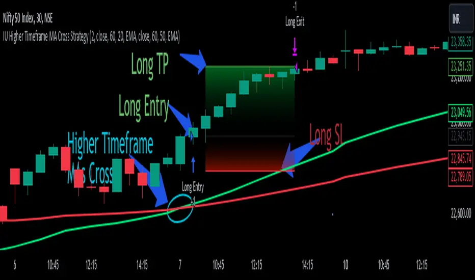
IU Higher Timeframe MA Cross StrategyIU Higher Timeframe MA Cross Strategy
The IU Higher Timeframe MA Cross Strategy is a versatile trading tool designed to identify trend by utilizing two customizable moving averages (MAs) across different timeframes and types. This strategy includes detailed entry and exit rules with fully configurable inputs, offering flexibility to suit various trading styles.
Key Features:
- Two moving averages (MA1 and MA2) with customizable types, lengths, sources, and timeframes.
- Both long and short trade setups based on MA crossovers.
- Integrated risk management with adjustable stop-loss and take-profit levels based on a user-defined risk-to-reward (RTR) ratio.
- Clear visualization of MAs, entry points, stop-loss, and take-profit zones.
Inputs:
1. Risk-to-Reward Ratio (RTR):
- Defines the take-profit level in relation to the stop-loss distance. Default is 2.
2. MA1 Settings:
- Source: Select the data source for calculating MA1 (e.g., close, open, high, low). Default is close.
- Timeframe: Specify the timeframe for MA1 calculation. Default is 60 (60-minute chart).
- Length: Set the lookback period for MA1 calculation. Default is 20.
- Type: Choose the type of moving average (options: SMA, EMA, SMMA, WMA, VWMA). Default is EMA.
- Smooth: Option to enable or disable smoothing of MA1 to merge gaps. Default is true.
3. MA2 Settings:
- Source: Select the data source for calculating MA2 (e.g., close, open, high, low). Default is close.
- Timeframe: Specify the timeframe for MA2 calculation. Default is 60 (60-minute chart).
- Length: Set the lookback period for MA2 calculation. Default is 50.
- Type: Choose the type of moving average (options: SMA, EMA, SMMA, WMA, VWMA). Default is EMA.
- Smooth: Option to enable or disable smoothing of MA2 to merge gaps. Default is true.
Entry Rules:
- Long Entry:
- Triggered when MA1 crosses above MA2 (crossover).
- Entry is confirmed only when the bar is closed and no existing position is active.
- Short Entry:
- Triggered when MA1 crosses below MA2 (crossunder).
- Entry is confirmed only when the bar is closed and no existing position is active.
Exit Rules:
- Stop-Loss:
- For long positions: Set at the low of the bar preceding the entry.
- For short positions: Set at the high of the bar preceding the entry.
- Take-Profit:
- For long positions: Calculated as (Entry Price - Stop-Loss) * RTR + Entry Price.
- For short positions: Calculated as Entry Price - (Stop-Loss - Entry Price) * RTR.
Visualization:
- Plots MA1 and MA2 on the chart with distinct colors for easy identification.
- Highlights stop-loss and take-profit levels using shaded zones for clear visual representation.
- Displays the entry level for active positions.
This strategy provides a robust framework for traders to identify and act on trend reversals while maintaining strict risk management. The flexibility of its inputs allows for seamless customization to adapt to various market conditions and trading preferences.
Kernel Regression Envelope with SMI OscillatorThis script combines the predictive capabilities of the **Nadaraya-Watson estimator**, implemented by the esteemed jdehorty (credit to him for his excellent work on the `KernelFunctions` library and the original Nadaraya-Watson Envelope indicator), with the confirmation strength of the **Stochastic Momentum Index (SMI)** to create a dynamic trend reversal strategy. The core idea is to identify potential overbought and oversold conditions using the Nadaraya-Watson Envelope and then confirm these signals with the SMI before entering a trade.
**Understanding the Nadaraya-Watson Envelope:**
The Nadaraya-Watson estimator is a non-parametric regression technique that essentially calculates a weighted average of past price data to estimate the current underlying trend. Unlike simple moving averages that give equal weight to all past data within a defined period, the Nadaraya-Watson estimator uses a **kernel function** (in this case, the Rational Quadratic Kernel) to assign weights. The key parameters influencing this estimation are:
* **Lookback Window (h):** This determines how many historical bars are considered for the estimation. A larger window results in a smoother estimation, while a smaller window makes it more reactive to recent price changes.
* **Relative Weighting (alpha):** This parameter controls the influence of different time frames in the estimation. Lower values emphasize longer-term price action, while higher values make the estimator more sensitive to shorter-term movements.
* **Start Regression at Bar (x\_0):** This allows you to exclude the potentially volatile initial bars of a chart from the calculation, leading to a more stable estimation.
The script calculates the Nadaraya-Watson estimation for the closing price (`yhat_close`), as well as the highs (`yhat_high`) and lows (`yhat_low`). The `yhat_close` is then used as the central trend line.
**Dynamic Envelope Bands with ATR:**
To identify potential entry and exit points around the Nadaraya-Watson estimation, the script uses **Average True Range (ATR)** to create dynamic envelope bands. ATR measures the volatility of the price. By multiplying the ATR by different factors (`nearFactor` and `farFactor`), we create multiple bands:
* **Near Bands:** These are closer to the Nadaraya-Watson estimation and are intended to identify potential immediate overbought or oversold zones.
* **Far Bands:** These are further away and can act as potential take-profit or stop-loss levels, representing more extreme price extensions.
The script calculates both near and far upper and lower bands, as well as an average between the near and far bands. This provides a nuanced view of potential support and resistance levels around the estimated trend.
**Confirming Reversals with the Stochastic Momentum Index (SMI):**
While the Nadaraya-Watson Envelope identifies potential overextended conditions, the **Stochastic Momentum Index (SMI)** is used to confirm a potential trend reversal. The SMI, unlike a traditional stochastic oscillator, oscillates around a zero line. It measures the location of the current closing price relative to the median of the high/low range over a specified period.
The script calculates the SMI on a **higher timeframe** (defined by the "Timeframe" input) to gain a broader perspective on the market momentum. This helps to filter out potential whipsaws and false signals that might occur on the current chart's timeframe. The SMI calculation involves:
* **%K Length:** The lookback period for calculating the highest high and lowest low.
* **%D Length:** The period for smoothing the relative range.
* **EMA Length:** The period for smoothing the SMI itself.
The script uses a double EMA for smoothing within the SMI calculation for added smoothness.
**How the Indicators Work Together in the Strategy:**
The strategy enters a long position when:
1. The closing price crosses below the **near lower band** of the Nadaraya-Watson Envelope, suggesting a potential oversold condition.
2. The SMI crosses above its EMA, indicating positive momentum.
3. The SMI value is below -50, further supporting the oversold idea on the higher timeframe.
Conversely, the strategy enters a short position when:
1. The closing price crosses above the **near upper band** of the Nadaraya-Watson Envelope, suggesting a potential overbought condition.
2. The SMI crosses below its EMA, indicating negative momentum.
3. The SMI value is above 50, further supporting the overbought idea on the higher timeframe.
Trades are closed when the price crosses the **far band** in the opposite direction of the trade. A stop-loss is also implemented based on a fixed value.
**In essence:** The Nadaraya-Watson Envelope identifies areas where the price might be deviating significantly from its estimated trend. The SMI, calculated on a higher timeframe, then acts as a confirmation signal, suggesting that the momentum is shifting in the direction of a potential reversal. The ATR-based bands provide dynamic entry and exit points based on the current volatility.
**How to Use the Script:**
1. **Apply the script to your chart.**
2. **Adjust the "Kernel Settings":**
* **Lookback Window (h):** Experiment with different values to find the smoothness that best suits the asset and timeframe you are trading. Lower values make the envelope more reactive, while higher values make it smoother.
* **Relative Weighting (alpha):** Adjust to control the influence of different timeframes on the Nadaraya-Watson estimation.
* **Start Regression at Bar (x\_0):** Increase this value if you want to exclude the initial, potentially volatile, bars from the calculation.
* **Stoploss:** Set your desired stop-loss value.
3. **Adjust the "SMI" settings:**
* **%K Length, %D Length, EMA Length:** These parameters control the sensitivity and smoothness of the SMI. Experiment to find settings that work well for your trading style.
* **Timeframe:** Select the higher timeframe you want to use for SMI confirmation.
4. **Adjust the "ATR Length" and "Near/Far ATR Factor":** These settings control the width and sensitivity of the envelope bands. Smaller ATR lengths make the bands more reactive to recent volatility.
5. **Customize the "Color Settings"** to your preference.
6. **Observe the plots:**
* The **Nadaraya-Watson Estimation (yhat)** line represents the estimated underlying trend.
* The **near and far upper and lower bands** visualize potential overbought and oversold zones based on the ATR.
* The **fill areas** highlight the regions between the near and far bands.
7. **Look for entry signals:** A long entry is considered when the price touches or crosses below the lower near band and the SMI confirms upward momentum. A short entry is considered when the price touches or crosses above the upper near band and the SMI confirms downward momentum.
8. **Manage your trades:** The script provides exit signals when the price crosses the far band. The fixed stop-loss will also close trades if the price moves against your position.
**Justification for Combining Nadaraya-Watson Envelope and SMI:**
The combination of the Nadaraya-Watson Envelope and the SMI provides a more robust approach to identifying potential trend reversals compared to using either indicator in isolation. The Nadaraya-Watson Envelope excels at identifying potential areas where the price is overextended relative to its recent history. However, relying solely on the envelope can lead to false signals, especially in choppy or volatile markets. By incorporating the SMI as a confirmation tool, we add a momentum filter that helps to validate the potential reversals signaled by the envelope. The higher timeframe SMI further helps to filter out noise and focus on more significant shifts in momentum. The ATR-based bands add a dynamic element to the entry and exit points, adapting to the current market volatility. This mashup aims to leverage the strengths of each indicator to create a more reliable trading strategy.

Korneev Reverse RSIRethinking the Legendary Relative Strength Index by John Welles Wilder
The essence of the new approach lies in the reverse use of the so-called "overbought" and "oversold" zones. In his 1978 book, "New Concepts in Technical Trading Systems," where the RSI mechanism was thoroughly described, Wilder writes that one way to use the oscillator is to open a long position when the RSI drops into oversold territory (below 30) and to open a short position when the RSI rises to overbought levels (above 70). However, backtesting this strategy with such inputs yields rather mediocre results.
Based on the calculation formula, the RSI calculates the rate of price change over a certain period. Therefore, overbought and oversold zones will have relative significance (relative to the set calculation period). It is no coincidence that the word "relative" was added to the name of the oscillator. It is worth accepting as an axiom the assertion that the price of an asset is fair at every moment in time.
Essentially, the RSI calculates the strength of a trend. If the oscillator value is above 70, it is highly likely that an upward movement is occurring in the market. Therefore, in the current strategy, a long position is opened precisely at the moment of greatest buyer strength (when RSI > 80), i.e., in the direction of the trend, since counter-trend trading with the RSI has proven to be ineffective. The position is closed after the buyers lose their advantage and the RSI drops to 40.
The strategy is recommended to be used only with long positions, as short positions show negative results. The strategy uses a moving average for the RSI with a period of 14 to smooth the oscillator data.
--------------------------------------------------------------------------------------------
Переосмысление легендарного осциллятора Relative strength index Джона Уэллса Уайлдера
Суть нового подхода заключается в реверсивном использовании так называемых зон "перекупленности" и "перепроданности". В своей книге от 1978 года "New concepts in tecnical trading systems", в которой был подробно описан механизм работы RSI, Уайлдер пишет, что один из способов использования осциллятора - открытие длинной позиции при снижении RSI в перепроданность (ниже 30) и открытие короткой позиции при повышении RSI до перекупленности (выше 70). Однако бэктест стратегии с такими вводными дает весьма посредственные результаты.
Исходя из формулы расчета, RSI рассчитывает скорость изменения цены за определенный период. Поэтому зоны перекупленности и перепроданности будут иметь относительное значение (относительно установленного периода расчета). Не зря ведь в названии осциллятора было добавлено слово "относительной". Стоит принять за аксиому утверждение, что цена актива справедлива в каждый момент времени.
По сути, RSI рассчитывает силу тренда. Если значение осциллятора выше 70, то на рынке с высокой долей вероятности происходит восходящее движение. Поэтому в текущей стратегии открытие лонга происходит именно в момент наибольшей силы покупателей (когда RSI > 80), то есть в сторону тренда, поскольку контртрендовая торговля по RSI показала свою несостоятельность. Закрытие позиции происходит после того, как покупатели теряют преимущество и RSI снижается до 40.
Стратегию рекомендуется использовать только с длинными позициями, поскольку короткие позиции показывают отрицательный результат. В стратегии используется скользящая средняя для RSI с периодом 14 для сглаживания данных осциллятора.

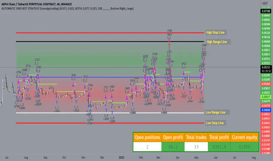
AUTOMATIC GRID BOT STRATEGY [ilovealgotrading]
OVERVIEW:
This Grid trading strategy can help you maximize your profit in a ranging sideways market with no clear direction.
INDICATOR:
We can get some money by taking advantage of the movement of the price between the range we have determined.
Short positions are opened while the price is rising, long positions are opened while the price is falling.
Therefore, there is no need to predict the trend direction.
What is different in this indicator:
I want to say thank you to © thequantscience. His GRID SPOT TRADING ALGORITHM - GRID BOT TRADING strategy helped me when I was writing my indicator.
I want to explain what I have improved:
1- Grid strategy is a type of strategy that can be traded in very short time frames and users can trade this strategy algorithmically by connecting this strategy to their own accounts with the help of API systems. For this reason, I have developed a software that can give us signals by dynamically changing the long and short messages when users are trading.
2- We can change the start and end dates of our grid bot as we want. It is necessary to use this setting when setting up automatic bots, so that previously opened transactions are not taken into account.
3 - Lot or quantity size should not be excessively small when users are taking automatic trades because exchanges have limitations, to avoid this problem, I have prevented this error by automatically rounding up to the nearest quantity size inside the software.
4 - Users can avoid excessive losses by using stop loss on this grid bot if they wish.
5 - When our price is over the range high or below the range low, our open positions are closed, if the stop button is active. We can also change which close price time frame we take as a basis from the settings.
6 -Users can set how many dollars they can enter per transaction while performing their transactions automatically.
IMPLEMENTATION DETAILS – SETTINGS:
This script allows the user to choose the highs and lows leves of our range. Our bot trades in the specified range.
1. This strategy allows us to set start and end backtest dates.
2. We can change range high and range low leves of our bot
3. IF people want to trade algorithmically with the help of this bot, there are 6 different input systems that will receive the Json codes as an alarm
4. IF the price closes above the upper line or below the lower line, all transactions will be closed. We can determine in which time frame our transactions will be stopped if the price closes outside these levels.We can adjust how our bot works by activating or turning off the Stop Loss button.
5. In this strategy, you can determine your dollar cost for per position.
6. The user can also divide the interval we have determined into 10 parts or 20 equal parts.
7. The grid is divided and colored at the interval we set. At the same time, if we don't want we can turn off colored channels.
Notes:
If you're going to connect this bot to an automatic Long and Short direction,
Don’t forget! you need to Webhook URL,
Don’t miss paste this code to your message window {{strategy.order.alert_message}}
ALSO:
Set your range below the support zones and above the resistance zones.
Don't be afraid to take a wide range, it doesn't matter if you make a little money, the important thing is that you don't lose money.
If you have any ideas what to add to my work to add more sources or make calculations cooler, suggest in DM .
Kitchen [ilovealgotrading]
OVERVIEW:
Kitchen is a strategy that aims to trade in the direction of the trend by using supertrend and stochRsi data by calculating at different time values.
IMPLEMENTATION DETAILS – SETTINGS:
First of all, let's understand the supertrend and stocrsi indicators.
How do you read and use Super Trend for trading ?
The price is often going upwards when it breaks the super trend line while keeping its position above the indication level.
When the market is in a bullish trend, the indicator becomes green. The indicator level will act as trendline support in such a scenario. The color of the indicator changes to red to indicate a negative trend once the price crosses the support line. The price uses the super trend level as a trendline resistance during a bearish move.
In our strategy, if our 1-hour and 4-hour supertrend lines show the up or down train in the same direction at the same time, we can assume that a train is forming here.
Why do I use the time of 1 hour and 4 hours ?
When I did a backtest from the past to the present, I discovered that the most accurate and consistent time zones are the 1 hour and 4 hour time zones.
By the way we can change our short term timeframe(1H) and long term timeframe(4H) from settings panel.
How do you read and use the Stoch-RSI Indicator?
This indicator analyzes price dynamics automatically to detect overbought and oversold locations.
The indicator includes:
- The primary line, which typically has values between 0 and 100;
- Two dynamic levels for overbought and oversold conditions.
IF our stoch-rsi indicator value has fallen below our lower boundary line, the oversold event has been observed in the price, if our stoch-rsi value breaks up our bottom line after becoming oversold, we think that the price will start the recovery phase.(The case is also true for the opposite.)
However, this does not always apply and we need additional approvals, Therefore, our 1H and 4H supertrrend indicator provides us with additional confirmation.
Buy Condition:
Our 1H(short term) and 4H(long term) supertrrend indicator, has given the buy signal(green line and yellow line), and if our stochrsi indicator has broken our oversold line up on the past 15 bars, the buy signal is formed here.
Sell Condition:
Our 1H(short term) and 4H(long term) supertrrend indicator, has given the sell signal(red line and orange line), and if our stochrsi indicator has broken our overbuy line down on the past 15 bars, the sell signal is formed here.
Stop Loss or Take Profit Conditions:
Exit Long Senerio:
All conditions are completed, the buy signal has arrived and we have entered a LONG trade, the 1-hour supertrend line follows the price rise(yellow line), if the price breaks below the 1-hour super trend line and a sell condition occurs for 1H timeframe for supertrend indcator, LONG trade will exit here.
Exit Short Senerio:
All conditions are completed, the Sell signal has arrived and we have entered a SHORT trade, the 1-hour supertrend line follows the price down(orange line), if the price breaks up the 1-hour super trend line and a buy condition occurs for 1H timeframe for supertrend indcator, SHORT trade will exit here.
What can you change in the settings panel?
1-We can set Start and End date for backtest and future alarms
2-We can set ATR length and Factor for supertrend indicator
3-We can set our short term and long term timeframe value
4-We can set StochRsi Up and Low limit to confirm buy and sell conditions
5-We can set stochrsi retroactive approval length
6-We can set stochrsi values or the length
7-We can set Dollar cost for per position
8- We can choose the direction of our positions, we can set only LONG, only SHORT or both directions.
9-IF you want to place automatic buy and sell orders with this strategy, you can paste your codes into the Long open-close or Short open-close message sections.
For example
IF you write your alert window this code {{strategy.order.alert_message}}.
When trigger Long signal you will get dynamically what you pasted here for Long Open Message
ALSO:
Please do not open trades without properly managing your risk and psychology!!!
If you have any ideas what to add to my work to add more sources or make calculations cooler, suggest in DM .

Bollinger Bands %B - Belt Holds & Inner CandlesThis is a simple strategy that uses Bollinger Bands %B represented as a histogram combined with Candle Beltholds and Inside candles for entry signals, and combines this with "buy" and "sell" zones of the %B indicator, to buy and sell based on the zones you set.
How to use:
Long when in the green zone and an inside candle (which is highlighted in white) or a bullish belt hold (which is highlighted in yellow), and sell when inside a red zone and has an inside candle or a bearish belt hold (which is highlighted in purple) or the stop loss or take profit is hit.
Short when in the red zone and an inside candle (which is highlighted in white) or a bearish belt hold (which is highlighted in purple), and sell when inside a green zone and has an inside candle or a bullish belt hold (which is highlighted in yellow) or the stop loss or take profit is hit.
Stop loss / take profit selection:
Choose which performs best for you, ATR based uses the average true range, and % based is based on a set percent of loss or profit.

Session Opening Range Breakout (ORBO)This strategy automates a classic Opening Range Breakout (ORBO) approach: it builds a price range for the first minutes after the market opens, then looks for strong breakouts above or below that range to catch early directional moves.
Concept
The idea behind ORBO is simple:
The first minutes after the session open are often highly informative.
Price forms an “opening range” that acts as a mini support/resistance zone.
A clean breakout beyond this zone can lead to high-momentum moves.
This script turns that logic into a fully backtestable strategy in TradingView.
How the strategy works
Opening Range Session
Default session: 09:30–09:50 (exchange time)
During this window, the script tracks:
orHigh → highest high within the session
orLow → lowest low within the session
This forms your Opening Range for the day.
Breakout Logic (after the window ends)
Once the defined session ends:
Long Entry:
If the close crosses above the Opening Range High (orHigh),
→ strategy.entry("OR Long", strategy.long) is triggered.
Short Entry:
If the close crosses below the Opening Range Low (orLow),
→ strategy.entry("OR Short", strategy.short) is triggered.
Only one opening range per day is considered, which keeps the logic clean and easy to interpret.
Daily Reset
At the start of a new trading day, the script resets:
orHigh := na
orLow := na
A fresh Opening Range is then built using the next session’s 09:30–09:50 candles.
This ensures entries are always based on today’s structure, not yesterday’s.
Visuals & Inputs
Inputs:
Opening range session → default: "0930-0950"
Show OR levels → toggle visibility of OR High / Low lines
Fill range body → optional shaded zone between OR High and OR Low
Chart visuals:
A green line marks the Opening Range High.
A red line marks the Opening Range Low.
Optional yellow fill highlights the entire OR zone.
Background shading during the session shows when the range is currently being built.
These visuals make it easy to see:
Where the OR sits relative to current price
How clean / noisy the breakout was
How often price respects or rejects the opening zone
Backtesting & Optimization
Because this is written as a strategy():
You can use TradingView’s Strategy Tester to view:
Win rate
Net profit
Drawdown
Profit factor
Equity curve
Ideas to experiment with:
Change the session window (e.g., 09:15–09:45, 10:00–10:30)
Apply to different:
Markets: indices, FX, crypto, stocks
Timeframes: 1m / 5m / 15m
Add your own:
Stop Loss & Take Profit levels
Time filters (only trade certain days / times)
Volatility filters (e.g., ATR, range size thresholds)
Higher-timeframe trend filter (e.g., only take longs above 200 EMA)

Hilega Milega v6 - Pure EMA/SMA (Nitesh Kumar) + Full BacktestHilega to milega
he Hilega Milega Strategy, inspired by the technique of Nitesh Kumar, is designed for intraday and swing traders who want structured entries and exits with clear demand–supply logic.
🔑 Core Features
Demand & Supply Zones – Automatically plots potential strong buying and selling zones for high-probability trades.
Trend Identification – Uses a blend of EMAs/SMA crossovers to identify bullish and bearish market bias.
Buy & Sell Signals – Generates real-time visual signals based on “Hilega Milega” rules for quick decision-making.
Risk Management – Suggested stop-loss levels are derived from recent demand–supply areas to minimize drawdowns.
Backtesting Enabled – Traders can test the performance across multiple assets (stocks, forex, crypto, commodities).
📊 How It Works
Buy Signal → When price action confirms a bullish zone with supporting trend filters.
Sell Signal → When price action confirms a bearish zone or reversal pattern.
Flat/Exit → Position closed when opposite signal triggers or demand–supply imbalance fades.
⚡ Best Use Cases
Intraday trading (5m, 15m, 1H charts).
Swing trading (4H, Daily charts).
Works across stocks, crypto, commodities, and forex.
⚠️ Disclaimer: This strategy is for educational purposes. Backtest thoroughly and apply proper risk management before live trading.

[Stratégia] VWAP Mean Magnet v9 (Simple Alert)This strategy is specifically designed for a ranging (sideways-moving) Bitcoin market.
A trade is only opened and signaled on the chart if all three of the following conditions are met simultaneously at the close of a candle:
Zone Entry
The price must cross into the signal zone: the red band for a Short (sell) position, or the green band for a Long (buy) position.
RSI Confirmation
The RSI indicator must also confirm the signal. For a Short, it must go above 65 (overbought condition). For a Long, it must fall below 25 (oversold condition).
Volume Filter
The volume on the entry candle cannot be excessively high. This safety filter is designed to prevent trades during risky, high-momentum breakouts.

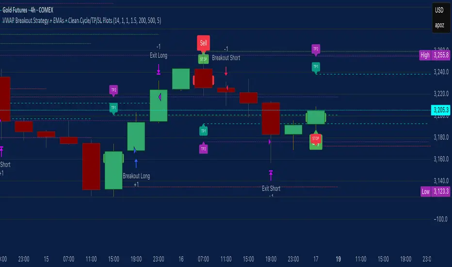
VWAP Breakout Strategy + EMAs + Clean Cycle/TP/SL PlotsHere’s a quick user-guide to get you up and running with your “VWAP Breakout Strategy + EMAs + Clean Cycle/TP/SL Plots” script in TradingView:
⸻
1. Installing the Script
1. Open TradingView, go to Pine Editor (bottom panel).
2. Paste in your full Pine-v6 code and hit Add to chart.
3. Save it (“Save as…”): give it a memorable name (e.g. “VWAP Breakout+EMAs”).
⸻
2. Configuring Your Inputs
Once it’s on the chart, click the ⚙️ Settings icon to tune:
Setting Default What it does
ATR Length 14 Period for average true range (volatility measure)
ATR Multiplier for Stop 1.5 How many ATRs away your stop-loss sits
TP1 / TP2 Multipliers (ATR) 1.0 / 2.0 Distance of TP1 and TP2 in ATR multiples
Show VWAP / EMAs On Toggles the blue VWAP line & EMAs (100/34/5)
Full Cycle Range Points 200 Height of the shaded “cycle zone”
Pivot Lookback 5 How many bars back to detect a pivot low
Round Number Step 500 Spacing of your dotted horizontal lines
Show TP/SL Labels On Toggles all the “ENTRY”, “TP1”, “TP2”, “STOP” tags
Feel free to adjust ATR multipliers and cycle-zone size based on the instrument’s typical range.
⸻
3. Reading the Signals
• Long Entry:
• Trigger: price crosses above VWAP
• You’ll see a green “Buy” tag at the low of the signal bar, plus an “ENTRY (Long)” label at the close.
• Stop is plotted as a red dashed line below (ATR × 1.5), and TP1/TP2 as teal and purple lines above.
• Short Entry:
• Trigger: price crosses below VWAP
• A red “Sell” tag appears at the high, with “ENTRY (Short)” at the close.
• Stop is the green line above; TP1/TP2 are dashed teal/purple lines below.
⸻
4. Full Cycle Zone
Whenever a new pivot low is detected (using your Pivot Lookback), the script deletes the old box and draws a shaded yellow rectangle from that low up by “Full Cycle Range Points.”
• Use this to visualize the “maximum expected swing” from your pivot.
• You can quickly see whether price is still traveling within a normal cycle or has overstretched.
⸻
5. Round-Number Levels
With Show Round Number Levels enabled, you’ll always get horizontal dotted lines at the nearest multiples of your “Round Number Step” (e.g. every 500 points).
• These often act as psychological support/resistance.
• Handy to see confluence with VWAP or cycle-zone edges.
⸻
6. Tips & Best-Practices
• Timeframes: Apply on any intraday chart (5 min, 15 min, H1…), but match your ATR length & cycle-points to the timeframe’s typical range.
• Backtest first: Use the Strategy Tester tab to review performance, tweak ATR multipliers or cycle size, then optimize.
• Combine with context: Don’t trade VWAP breakouts blindly—look for confluence (e.g. support/resistance zones, higher-timeframe trend).
• Label clutter: If too many labels build up, you can toggle Show TP/SL Labels off and rely just on the lines.
⸻
That’s it! Once you’ve added it to your chart and dialed in the inputs, your entries, exits, cycle ranges, and key levels will all be plotted automatically. Feel free to experiment with the ATR multipliers and cycle-zone size until it fits your instrument’s personality. Happy trading!
Multi-Band Comparison Strategy (CRYPTO)Multi-Band Comparison Strategy (CRYPTO)
Optimized for Cryptocurrency Trading
This Pine Script strategy is built from the ground up for traders who want to take advantage of cryptocurrency volatility using a confluence of advanced statistical bands. The strategy layers Bollinger Bands, Quantile Bands, and a unique Power-Law Band to map out crucial support/resistance zones. It then focuses on a Trigger Line—the lower standard deviation band of the upper quantile—to pinpoint precise entry and exit signals.
Key Features
Bollinger Band Overlay
The upper Bollinger Band visually shifts to yellow when price exceeds it, turning black otherwise. This offers a straightforward way to gauge heightened momentum or potential market slowdowns.
Quantile & Power-Law Integration
The script calculates upper and lower quantile bands to assess probabilistic price extremes.
A Power-Law Band is also available to measure historically significant return levels, providing further insight into overbought or oversold conditions in fast-moving crypto markets.
Standard Deviation Trigger
The lower standard deviation band of the upper quantile acts as the strategy’s trigger. If price consistently holds above this line, the strategy interprets it as a strong bullish signal (“green” zone). Conversely, dipping below indicates a “red” zone, signaling potential reversals or exits.
Consecutive Bar Confirmation
To reduce choppy signals, you can fine-tune the number of consecutive bars required to confirm an entry or exit. This helps filter out noise and false breaks—critical in the often-volatile crypto realm.
Adaptive for Multiple Timeframes
Whether you’re scalping on a 5-minute chart or swing trading on daily candles, the strategy’s flexible confirmation and overlay options cater to different market conditions and trading styles.
Complete Plot Customization
Easily toggle visibility of each band or line—Bollinger, Quantile, Power-Law, and more.
Built-in Simple and Exponential Moving Averages can be enabled to further contextualize market trends.
Why It Excels at Crypto
Cryptocurrencies are known for rapid price swings, and this strategy addresses exactly that by combining multiple statistical methods. The quantile-based confirmation reduces noise, while Bollinger and Power-Law bands help highlight breakout regions in trending markets. Traders have reported that it works seamlessly across various coins and tokens, adapting its triggers to each asset’s unique volatility profile.
Give it a try on your favorite cryptocurrency pairs. With advanced data handling, crisp visual cues, and adjustable confirmation logic, the Multi-Band Comparison Strategy provides a robust framework to capture profitable moves and mitigate risk in the ever-evolving crypto space.
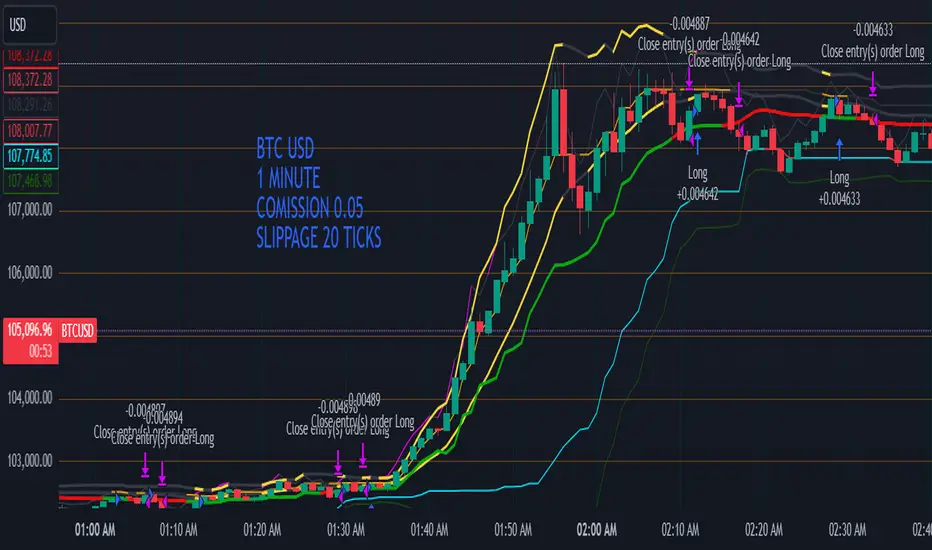
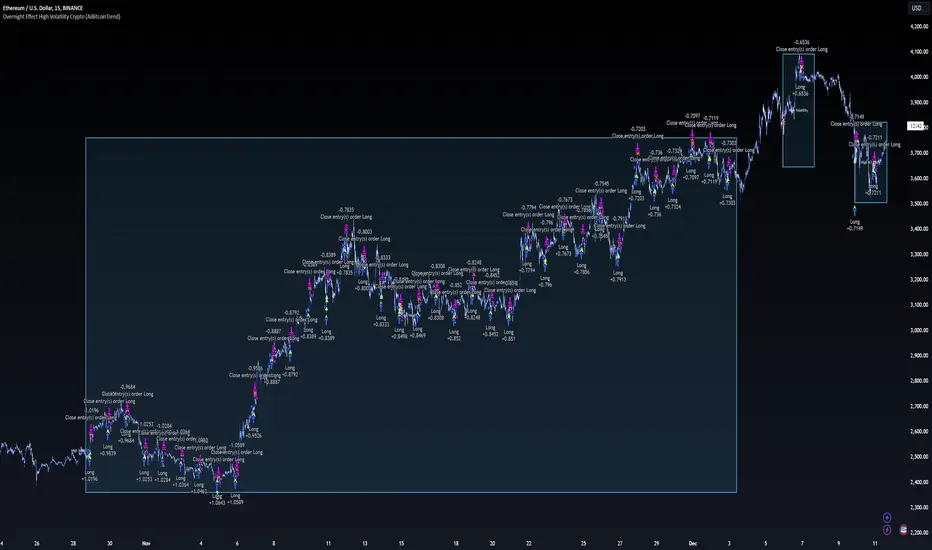
Overnight Effect High Volatility Crypto (AiBitcoinTrend)👽 Overview of the Strategy
This strategy leverages the overnight effect in the cryptocurrency market, specifically targeting the two-hour window from 21:00 UTC to 23:00 UTC. The strategy is designed to be applied only during periods of high volatility, which is determined using historical volatility data. This approach, inspired by research from Padyšák and Vojtko (2022), aims to capitalize on statistically significant return patterns observed during these hours.
Deep Backtesting with a High Volatility Filter
Deep Backtesting without a High Volatility Filter
👽 How the Strategy Works
Volatility Calculation:
Each day at 00:00 UTC, the strategy calculates the 30-day historical volatility of crypto returns (typically Bitcoin). The historical volatility is the standard deviation of the log returns over the past 30 days, representing the market's recent volatility level.
Median Volatility Benchmark:
The median of the 30-day historical volatility is calculated over a 365-day period (one year). This median acts as a benchmark to classify each day as either:
👾 High Volatility: When the current 30-day volatility exceeds the median volatility.
👾 Low Volatility: When the current 30-day volatility is below the median.
Trading Rule:
If the day is classified as a High Volatility Day, the strategy executes the following trades:
👾 Buy at 21:00 UTC.
👾 Sell at 23:00 UTC.
Trade Execution Details:
The strategy uses a 0.02% fee per trade.
Each trade is executed with 25% of the available capital. This allocation helps manage risk while allowing for compounding returns.
Rationale:
The returns during the 22:00 and 23:00 UTC hours have been found to be statistically significant during high volatility periods. The overnight effect is believed to drive this phenomenon due to the asynchronous closing hours of global financial markets. This creates unique trading opportunities in the cryptocurrency market, where exchanges remain open 24/7.
👽 Market Context and Global Time Zone Impact
👾 Why 21:00 to 23:00 UTC?
During this window, major traditional financial markets are closed:
NYSE (New York) closes at 21:00 UTC.
London and European markets are closed during these hours.
Asian markets (Tokyo, Hong Kong, etc.) open later, leaving this window largely unaffected by traditional trading flows.
This global market inactivity creates a period where significant moves can occur in the cryptocurrency market, particularly during high volatility.
👽 Strategy Parameters
Volatility Period: 30 days.
The lookback period for calculating historical volatility.
Median Period: 365 days.
The lookback period for calculating the median volatility benchmark.
Entry Time: 21:00 UTC.
Adjust this to your local time if necessary (e.g., 16:00 in New York, 22:00 in Stockholm).
Exit Time: 23:00 UTC.
Adjust this to your local time if necessary (e.g., 18:00 in New York, 00:00 midnight in Stockholm).
👽 Benefits of the Strategy
Seasonality Effect:
The strategy captures consistent patterns driven by the overnight effect and high volatility periods.
Risk Reduction:
Since trades are executed during a specific window and only on high volatility days, the strategy helps mitigate exposure to broader market risk.
Simplicity and Efficiency:
The strategy is moderately complex, making it accessible for traders while offering significant returns.
Global Applicability:
Suitable for traders worldwide, with clear guidelines on adjusting for local time zones.
👽 Considerations
Market Conditions: The strategy works best in a high-volatility environment.
Execution: Requires precise timing to enter and exit trades at the specified hours.
Time Zone Adjustments: Ensure you convert UTC times accurately based on your location to execute trades at the correct local times.
Disclaimer: This information is for entertainment purposes only and does not constitute financial advice. Please consult with a qualified financial advisor before making any investment decisions.
LUBEThis is a chart meant for 30m BTCUSD but could be used for many other assets, and there are inputs to play with.
I decided on the strange title "LUBE" because I was measuring how many of the previous 500 bars had the current price level already been in. I wanted to discover when the price was in a new zone or an area that it hadn't spent much time in recently... the LUBE zone.
Think of the blue line as showing you the current level friction. If the blue line is high, price is quagmired and not moving quickly. Price could trend sideways for a while before breaking out. A high blue line is a high traffic zone for trading. When the blue line dips low, it's encountering a price zone the asset has not been observed in recently, and this could mean price could break out and move more freely and quickly when it does. We get a trade entry signal if the blue line dips below the bottom white line. The bottom white line is currently set to -10. Think about the lowest the blue line has been recently as 0, and the highest as 100. It is set by default (for BTCUSD 30m chart) to -10 meaning the blue line has to dip a little (-10%) below the lowest it has experienced recently to initiate a trade. This is the LUBE zone. The bottom white line shows that level. Again this is a level lower than the lowest amount of friction experienced in price action for the last 100 bars, but offset by 5 bars showing where that level was at 5 bars ago. We want to dip below that to initiate a trade.
The direction to trade in is determined by a very quick moving weighted moving average (variable name is "fir") to see if the recent trend is up or down. To end a trade, an arbitrary number between 0 and 100 is picked telling us when we are experiencing enough friction again to end the trade. I have it preset to 50 (think of it as 50/100 or half way between the white bars. At a 50% friction level it's time to get out of the trade.
Some shortcomings are missing the bulk of big moves, and experiencing whipsaws where price action zips up and then comes straight back down. Overall the backtest looks sweet enough to use on 2x leverage, experiencing a 17.78% max drawdown at the time of publishing. I wouldn't push the leverage any higher.
To get alerts change the word "strategy" to "study" and delete lines 60-67.
Bot traders using alerts: beware the alert conditions. If a trade goes directly from long to short (which happens rarely), without closing a trade first, it might not act properly. If you use bots to trade, for "LONG" please close any old trades first before putting in instructions to open a leveraged long. To go "SHORT" please remember to close any old trade first as well, and things *should* work out just fine.
Good luck, have fun, and feel free to mess up and butcher this code to your own liking. I'm not responsible if anything bad that happens to you if you use this trading system, or for any bugs you may encounter.

Elliott Wave Full Fractal System v2.0Elliott Wave Full Fractal System v2.0 – Q.C. FINAL (Guaranteed R/R)
Elliott Wave Full Fractal System is a multi-timeframe wave engine that automatically labels Elliott impulses and ABC corrections, then builds a rule-based, ATR-driven risk/reward framework around the “W3–W4–W5” leg.
“Guaranteed R/R” here means every order is placed with a predefined stop-loss and take-profit that respect a minimum Reward:Risk ratio – it does not mean guaranteed profits.
Core Idea
This strategy turns a full fractal Elliott Wave labelling engine into a systematic trading model.
It scans fractal pivots on three wave degrees (Primary, Intermediate, Minor) to detect 5-wave impulses and ABC corrections.
A separate “Trading Degree” pivot stream, filtered by a 200-EMA trend filter and ATR-based dynamic pivots, is then used to find W4 pullback entries with a minimum, user-defined Reward:Risk ratio.
Default Properties & Risk Assumptions
The backtest uses realistic but conservative defaults:
// Default properties used for backtesting
strategy(
"Elliott Wave Full Fractal System - Q.C. FINAL (Guaranteed R/R)",
overlay = true,
initial_capital = 10000, // realistic account size
default_qty_type = strategy.percent_of_equity,
default_qty_value = 1, // 1% risk per trade
commission_type = strategy.commission.cash_per_contract,
commission_value = 0.005, // example stock commission
slippage = 0 // see notes below
)
Account size: 10,000 (can be changed to match your own account).
Position sizing: 1% of equity per trade to keep risk per idea sustainable and aligned with TradingView’s recommendations.
Commission: 0.005 cash per contract/share as a realistic example for stock trading.
Slippage: set to 0 in code for clarity of “pure logic” backtesting. Real-life trading will experience slippage, so users should adjust this according to their market and broker.
Always re-run the backtest after changing any of these values, and avoid using high risk fractions (5–10%+) as that is rarely sustainable.
1. Full Fractal Wave Engine
The script builds and maintains four pivot streams using ATR-adaptive fractals:
Primary Degree (Macro Trend):
Captures the large swings that define the major trend. Labels ①–⑤ and ⒶⒷⒸ using blue “Circle” labels and thicker lines.
Intermediate Degree (Trading Degree):
Captures the medium swings (swing-trading horizon). Uses teal labels ( (1)…(5), (A)(B)(C) ).
Minor Degree (Micro Structure):
Tracks short-term swings inside the larger waves. Uses red roman numerals (i…v, a b c).
ABC Corrections (Optional):
When enabled, the engine tries to detect standard A–B–C corrective structures that follow a completed 5-wave impulse and plots them with dashed lines.
Each degree uses a dynamic pivot lookback that expands when ATR is above its EMA, so the system naturally requires “stronger” pivots in volatile environments and reacts faster in quiet conditions.
2. Theory Rules & Strict Mode
Normal Mode: More permissive detection. Designed to show more wave structures for educational / exploratory use.
Strict Mode: Enforces key Elliott constraints:
Wave 3 not shorter than waves 1 and 5.
No invalid W4 overlap with W1 (for standard impulses).
ABC Logic: After a confirmed bullish impulse, the script expects a down-up-down corrective pattern (A,B,C). After a bearish impulse, it looks for up-down-up.
3. Trend Filter & Pivots
EMA Trend Filter: A configurable EMA (default 200) is used as a non-wave trend filter.
Price above EMA → Only long setups are considered.
Price below EMA → Only short setups are considered.
ATR-Adaptive Pivots: The pivot engine scales its left/right bars based on current ATR vs ATR EMA, making waves and trading pivots more robust in volatile regimes.
4. Dynamic Risk Management (Guaranteed R/R Engine)
The trading engine is designed around risk, not just pattern recognition:
ATR-Based Stop:
Stop-loss is placed at:
Entry ± ATR × Multiplier (user-configurable, default 2.0).
This anchors risk to current volatility.
Minimum Reward:Risk Ratio:
For each setup, the script:
Computes the distance from entry to stop (risk).
Projects a take-profit target at risk × min_rr_ratio away from entry.
Only accepts the setup if risk is positive and the required R:R ratio is achievable.
Result: Every order is created with both TP and SL at a predefined distance, so each trade starts with a known, minimum Reward:Risk profile by design.
“Guaranteed R/R” refers exclusively to this order placement logic (TP/SL geometry), not to win-rate or profitability.
5. Trading Logic – W3–W4–W5 Pattern
The Trading pivot stream (separate from visual wave degrees) looks for a simple but powerful pattern:
Bullish structure:
Sequence of pivots forms a higher-high / higher-low pattern.
Price is above the EMA trend filter.
A strong “W3” leg is confirmed with structure rules (optionally stricter in Strict mode).
Entry (Long – W4 Pullback):
The “height” of W3 is measured.
Entry is placed at a configurable Fibonacci pullback (default 50%) inside that leg.
ATR-based stop is placed below entry.
Take-profit is projected to satisfy min Reward:Risk.
Bearish structure:
Mirrored logic (lower highs/lows, price below EMA, W3 down, W4 retrace up, W5 continuation down).
Once a valid setup is found, the script draws a colored box around the entry zone and a label describing the type of signal (“LONG SETUP” or “SHORT SETUP”) with the suggested limit price.
6. Orders & Execution
Entry Orders: The strategy uses limit orders at the computed W4 level (“Sniper Long” or “Sniper Short”).
Exits: A single strategy.exit() is attached to each entry with:
Take-profit at the projected minimum R:R target.
Stop-loss at ATR-based level.
One Trade at a Time: New setups are only used when there is no open position (strategy.opentrades == 0) to keep the logic clear and risk contained.
7. Visual Guide on the Chart
Wave Labels:
Primary: ①,②,③,④,⑤, ⒶⒷⒸ
Intermediate: (1)…(5), (A)(B)(C)
Minor: i…v, a b c
Trend EMA: Single blue EMA showing the dominant trend.
Setup Boxes:
Green transparent box → long entry zone.
Red transparent box → short entry zone.
Labels: “LONG SETUP / SHORT SETUP” labels mark the proposed limit entry with price.
8. How to Use This Strategy
Attach the strategy to your chart
Choose your market (stocks, indices, FX, crypto, futures, etc.) and timeframe (for example 1h, 4h, or Daily). Then add the strategy to the chart from your Scripts list.
Start with the default settings
Leave all inputs on their defaults first. This lets you see the “intended” behaviour and the exact properties used for the published backtest (account size, 1% risk, commission, etc.).
Study the wave map
Zoom in and out and look at the three wave degrees:
Blue circles → Primary degree (big picture trend).
Teal (1)…(5) → Intermediate degree (swing structure).
Red i…v → Minor degree (micro waves).
Use this to understand how the engine is interpreting the Elliott structure on your symbol.
Watch for valid setups
Look for the coloured boxes and labels:
Green box + “LONG SETUP” label → potential W4 pullback long in an uptrend.
Red box + “SHORT SETUP” label → potential W4 pullback short in a downtrend.
Only trades in the direction of the EMA trend filter are allowed by the strategy.
Check the Reward:Risk of each idea
For each setup, inspect:
Limit entry price.
ATR-based stop level.
Projected take-profit level.
Make sure the minimum Reward:Risk ratio matches your own rules before you consider trading it.
Backtest and evaluate
Open the Strategy Tester:
Verify you have a decent sample size (ideally 100+ trades).
Check drawdowns, average trade, win-rate and R:R distribution.
Change markets and timeframes to see where the logic behaves best.
Adapt to your own risk profile
If you plan to use it live:
Set Initial Capital to your real account size.
Adjust default_qty_value to a risk level you are comfortable with (often 0.5–2% per trade).
Set commission and slippage to realistic broker values.
Re-run the backtest after every major change.
Use as a framework, not a signal machine
Treat this as a structured Elliott/R:R framework:
Filter signals by higher-timeframe trend, major S/R, volume, or fundamentals.
Optionally hide some wave degrees or ABC labels if you want a cleaner chart.
Combine the system’s structure with your own trade management and discretion.
Best Practices & Limitations
This is an approximate Elliott Wave engine based on fractal pivots. It does not replace a full discretionary Elliott analysis.
All wave counts are algorithmic and can differ from a manual analyst’s interpretation.
Like any backtest, results depend heavily on:
Symbol and timeframe.
Sample size (more trades are better).
Realistic commission/slippage settings.
The 0-slippage default is chosen only to show the “raw logic”. In real markets, slippage can significantly impact performance.
No strategy wins all the time. Losing streaks and drawdowns will still occur even with a strict R:R framework.
Disclaimer
This script is for educational and research purposes only and does not constitute financial advice or a recommendation to buy or sell any security. Past performance, whether real or simulated, is not indicative of future results. Always test on multiple symbols/timeframes, use conservative risk, and consult your financial advisor before trading live capital.

Stratégie SMC V18.2 (BTC/EUR FINAL R3 - Tendance)This strategy is an automated implementation of Smart Money Concepts (SMC), designed to operate on the Bitcoin/Euro (BTC/EUR) chart using the 15-minute Timeframe (M15).It focuses on identifying high-probability zones (Order Blocks) after a confirmed Break of Structure (BOS) and a Liquidity Sweep, utilizing an H1/EMA 200 trend filter to only execute trades in the direction of the dominant market flow.Risk management is strict: every trade uses a fixed Risk-to-Reward Ratio (R:R) of 1:3.🧱 Core Logic Components
1. Trend Filter (H1/EMA 200)Objective: To avoid counter-trend entries, which has allowed the success rate to increase to nearly $65\%$ in backtests.Mechanism: A $200$-period EMA is plotted on a higher timeframe (Default: H1/60 minutes).Long (Buy): Entry is only permitted if the current price (M15) is above the trend EMA.Short (Sell): Entry is only permitted if the current price (M15) is below the trend EMA.
2. Order Block (OB) DetectionA potential Order Block is identified on the previous candle if it is
accompanied by an inefficiency (FVG - Fair Value Gap).
3. Advanced SMC ValidationBOS (Break of Structure): A recent BOS must be confirmed by breaking the swing high/low defined by the swing length (Default: 4 M15 candles).Liquidity (Liquidity Sweep): The Order Block zone must have swept recent liquidity (defined by the Liquidity Search Length) within a certain tolerance (Default: $0.1\%$).Point of Interest: The OB must form in a premium zone (for shorts) or a discount zone (for longs) relative to the current swing range (above or below the $50\%$ level of the range).
4. Execution and Risk ManagementEntry: The trade is triggered when the price touches the active Order Block (mitigation).Stop Loss (SL): The SL is fixed at the low of the OB (for longs) or the high of the OB (for shorts).Take Profit (TP): The TP is strictly set at a level corresponding to 3 times the SL distance (R:R 1:3).Lot Sizing: The trade quantity is calculated to risk a fixed amount (Default: 2.00 Euros) per transaction, capped by a Lot Max and Lot Min defined by the user.
Input Parameters (Optimized for BTC/EUR M15)Users can adjust these parameters to modify sensitivity and risk profile. The default values are those optimized for the high-performing backtest (Profit Factor $> 3$).ParameterDescriptionDefault Value (M15)Long. Swing (BOS)Candle length used to define the swing (and thus the BOS).4Long. Recherche Liq.Number of candles to scan to confirm a liquidity sweep.7Tolérance Liq. (%)Price tolerance to validate the liquidity sweep (as a percentage of price).0.1Timeframe TendanceChart timeframe used for the EMA filter (e.g., 60 = H1).60 (H1)Longueur EMA TendancePeriods used for the trend EMA.200Lot Max (Quantité Max BTC)Maximum quantity of BTC the strategy is allowed to trade.0.01Lot Min Réel (Exigence Broker)Minimum quantity required by the broker/exchange.0.00001

15m ORB + FVG Strategy (ChadAnt)Core Logic
The indicator's logic revolves around three main phases:
1. Defining the 15-Minute Opening Range (ORB)
The script calculates the highest high (rangeHigh) and lowest low (rangeLow) that occurred during the first 15 minutes of the trading day.
This time window is defined by the sessionStr input, which defaults to 0930-0945 (exchange time).
The high and low of this range are plotted as small gray dots once the session ends (rangeSet = true).
2. Identifying a Fair Value Gap (FVG) Setup
After the 15-minute range is set, the indicator waits for a breakout of either the range high or range low.
A "Strict FVG breakout" requires two conditions on the first candle that closes beyond the range:
The candle before the breakout candle ( bars ago) must have been inside the range.
The breakout candle ( bar ago) must have closed outside the range.
A Fair Value Gap (FVG) must form on the most recent three candles (the current bar and the two previous bars).
Bullish FVG (Long Setup): The low of the current bar (low) is greater than the high of the bar two periods prior (high ). This FVG represents a price inefficiency that the trade expects to fill.
Bearish FVG (Short Setup): The high of the current bar (high) is less than the low of the bar two periods prior (low ).
If a valid FVG setup occurs, the indicator marks a pending setup and draws a colored box to highlight the FVG area (Green for Bullish FVG, Red for Bearish FVG).
3. Trade Entry and Management
If a pending setup is identified, the trade is structured as a re-entry trade into the FVG zone:
Entry Price: Set at the outer boundary of the FVG, which is the low of the current bar for a Long setup, or the high of the current bar for a Short setup.
Stop Loss (SL): Set at the opposite boundary of the FVG, which is the low for a Long setup, or the high for a Short setup.
The trade is triggered (tradeActive = true) once the price retraces to the pendingEntry level.
Risk/Reward (RR) Targets: Three Take Profit (TP) levels are calculated based on the distance between the Entry and Stop Loss:
$$\text{Risk} = | \text{Entry} - \text{SL} |$$
$$\text{TP}n = \text{Entry} \pm (\text{Risk} \times \text{RR}n)$$
where $n$ is 1, 2, or 3, corresponding to the input $\text{RR}1$, $\text{RR}2$, and $\text{RR}3$ values (defaults: 1.0, 1.5, and 2.0).
Trade Lines: Upon triggering, lines for the Entry, Stop Loss, and three Take Profit levels are drawn on the chart for a specified length (lineLength).
A crucial feature is the directional lock (highBroken / lowBroken):
If the price breaks a range level (e.g., simpleBrokeHigh) but without a valid FVG setup, the corresponding directional flag (e.g., highBroken) is set to true permanently for the day.
This prevents the indicator from looking for any subsequent trade setups in that direction for the rest of the day, suggesting that the initial move, without an FVG, exhausted the opportunity.
Open-source script
In true TradingView spirit, the creator of this script has made it open-source, so that traders can review and verify its functionality. Kudos to the author! While you can use it for free, remember that republishing the code is subject to our House Rules.
ChadAnt
Disclaimer
The information and publications are not meant to be, and do not constitute, financial, investment, trading, or other types of advice or recommendations supplied

TMB Invest - Smart Money Concept StrategyEnglish:
**Quick Overview**
The "TMB_SMC_Strategy_v1.1.3" combines a classic trend filter using two EMAs with contrarian RSI entries and simple SMC elements (Fair Value Gaps & Order Blocks). Stop-loss and take-profit orders are volatility-adaptive and controlled via the ATR. An integrated dashboard displays the setup status, stop-loss/take-profit levels, entry reference, and trend, RSI, and ATR values.
---
## Operating Principle
1. **Trend Filter:** A fast EMA (default 50) is compared to a slow EMA (default 200). Trading occurs only in the direction of the trend: long in uptrends, short in downtrends.
2. **Timing via RSI:** Contrarian entries within the trend. Go long when the RSI is below a buy level (default 40); Short when the RSI is above a sell level (standard 60).
3. **Structure Check (SMC Proxy):** An "FVG Touch" serves as additional confirmation that an inefficient price zone has been tested. Order blocks are visualized for guidance but are not a direct entry trigger.
4. **Risk Management via ATR:** Stop-loss and take-profit levels are set as multipliers of the current ATR (e.g., SL = 1×ATR, TP = 2×ATR). This allows target and risk distances to adjust to market volatility.
5. **Simple Position Logic:** Only one position is held at a time (no pyramiding). After entry, stop and limit orders (bracket exit) are automatically placed.
---
## Input Values
* **EMA Fast / EMA Slow:** Lengths of the moving averages for the trend filter.
* **RSI Length / Levels:** Length of the RSI as well as buy and sell thresholds (contra signals within the trend direction).
* **Take Profit (RR) / Stop Loss (RR):** ATR multipliers for TP and SL.
* **Show FVGs & Order Blocks:** Toggles the visual SMC elements (zones/boxes) on or off.
--
## Signals & Execution
* **Long Setup:** Uptrend (fast EMA above slow EMA) **and** RSI below the buy level **and** a current FVG signal in a bullish direction.
* **Short Setup:** Downtrend (fast EMA below slow EMA) **and** RSI above the sell level **and** a current FVG touch in a bearish direction.
* **Entry & Exit:** If the setup is met, the market is entered; stop-loss/take-profit orders are placed immediately according to ATR multiples.
--
## Visualization
* **EMAs:** The fast and slow EMAs are plotted to illustrate the trend.
* **FVGs:** Fair Value Gaps are drawn as semi-transparent boxes in the trend color and projected slightly into the future.
* **Order Blocks:** Potential order block zones from the previous candle are visually highlighted (for informational purposes only).
---
## Integrated Dashboard
A compact table dashboard (bottom left) displays:
* Current **Setup Status** (Long/Short active, Long/Short ready, No Setup),
* **Stop-Loss**, **Take-Profit**, and **Entry Reference**,
* **Trend Status** (Bull/Bear/Sideways),
* **RSI Value**, and **ATR Value**.
Active long/short positions are highlighted in color (green/red).
--
## Practical Guide
1. **Place on Chart** and select the desired timeframe.
2. **Calibrate Parameters** (EMA lengths, RSI levels, ATR multipliers) to match the market and timeframe.
3. **Backtest** across different market phases; prioritize robustness over maximum curve fit.
4. **Fine-Tuning:**
* Shorter EMAs are often useful intraday (e.g., 20/100 or 34/144).
* Adjust RSI levels to market characteristics (45/55 for aggressive trading, 30/70 for conservative trading).
* Increase or decrease ATR multipliers depending on volatility/trading style.
--
## Notes, Limitations & Extensions
* **FVG Definition:** The FVG detection used here is intentionally simplified. Those who prefer a more rigorous approach can switch to a 3-candle definition and fill levels.
* **Order Blocks:** These primarily serve as a guide. Integration into entry/exit logic (e.g., retests) is possible as an extension.
* **Backtest Realism:** Fills may differ from the displayed closing price. For greater accuracy, intrabar backtests or an entry indicator based on the average position price are conceivable.
* **Alerts:** Currently, no alert conditions are defined; these can be added for long/short setups and status messages.
* **Position Management:** By default, no scaling is performed. Partial sales, trailing stops, or multiple entries can be added.
---
## Purpose & Benefits
The strategy offers a clear, modular framework: trend filter (direction), RSI contra timing (entry), SMC proxy via FVG Touch (structure), and ATR-based exits (risk adaptation). This makes it robust, easy to understand, and highly extensible—both for discretionary traders who appreciate visual SMC elements and for systematic testers who prefer a clean, parameterizable foundation.
