TMT Support & Resistance - Hitesh NimjeTMT Support & Resistance - HiteshNimje Indicator
Overview
The TMT Support & Resistance indicator is a professional pivot point analysis tool that automatically calculates and displays key support and resistance levels across multiple timeframe perspectives. It offers various pivot point calculation methods and provides customizable visual elements for comprehensive technical analysis.
Key Features
Pivot Point Calculation Methods
1. Traditional Pivot Points
Standard pivot point calculation using Previous Period High, Low, and Close
Creates P, S1, S2, S3, R1, R2, R3 levels
Most widely used method for day trading and swing trading
2. Fibonacci Pivot Points
Incorporates Fibonacci retracement levels (38.2%, 61.8%)
Uses traditional pivot as base with Fibonacci extensions
Popular among traders following Fibonacci analysis
3. Woodie Pivot Points
Alternative calculation method with different weighting
Emphasizes opening price in calculations
Preferred by some intraday traders
4. Classic Pivot Points
Similar to traditional but with different level calculations
Balanced approach to support/resistance identification
Timeframe Options
* Auto: Automatically selects optimal timeframe based on chart timeframe
Intraday ≤15min → Daily
Intraday >15min → Weekly
Daily → Monthly
* Fixed Timeframes: Daily, Weekly, Monthly, Quarterly, Yearly
* Extended Periods: Biyearly, Triyearly, Quinquennially, Decennially
Level Management System
Support Levels (Blue Colored)
* TMT Support 1 (S1): First major support level
* TMT Support 2 (S2): Second support level
* TMT Support 3 (S3): Third support level
* TMT Support 4 (S4): Fourth support level (Traditional/Camarilla only)
* TMT Support 5 (S5): Fifth support level (Traditional/Camarilla only)
Resistance Levels (Black Colored)
* TMT Resistance 1 (R1): First major resistance level
* TMT Resistance 2 (R2): Second resistance level
* TMT Resistance 3 (R3): Third resistance level
* TMT Resistance 4 (R4): Fourth resistance level (Traditional/Camarilla only)
* TMT Resistance 5 (R5): Fifth resistance level (Traditional/Camarilla only)
Central Pivot (Orange Colored)
* Pivot Point (P): Central price level used for S/R calculations
Customization Options
Display Settings
* Show Labels: Toggle pivot level identification labels
* Show Prices: Display actual price values next to levels
* Labels Position: Choose between Left or Right positioning
* Line Width: Adjustable thickness (1-100 pixels) for all pivot lines
Data Source Options
* Use Daily-based Values:
ON: Uses official daily OHLC values for calculations
OFF: Uses intraday data with extended hours consideration
* Number of Pivots Back: Historical pivot display (1-200 levels)
Color Customization
* Individual color selection for each support/resistance level
* Default colors: Supports (Blue), Resistances (Black), Pivot (Orange)
* Full color picker integration for all levels
Technical Features
Smart Display Logic
* Intraday Charts: Automatically uses daily-based calculations when intraday data is insufficient
* Multi-timeframe Compatibility: Adapts to chart timeframe and pivot timeframe differences
* Extended Hours Handling: Incorporates extended trading hours when enabled on chart
Dynamic Level Management
* Real-time Updates: Levels update as new data becomes available
* Historical Tracking: Maintains configurable number of historical pivot periods
* Automatic Cleanup: Removes old pivot graphics when limit is exceeded
Visual Elements
* Time-based Lines: Lines extend across full time periods for clear visual reference
* Price Labels: Contextual information showing level names and prices
* Professional Styling: Clean, professional appearance suitable for any trading style
Use Cases
Day Trading Applications
* Session Management: Use daily pivots for intraday trading decisions
* Range Trading: Camarilla levels excellent for range-bound strategies
* Breakout Confirmation: Use pivot breaks as entry/exit signals
Swing Trading Applications
* Weekly/Monthly Pivots: Identify key levels for multi-day positions
* Trend Analysis: Track how price interacts with higher timeframe pivots
* Risk Management: Set stop-losses and take-profits at pivot levels
Long-term Trading Applications
* Quarterly/Yearly Pivots: Major institutional levels for position trading
* Support/Resistance Maps: Create comprehensive price level roadmap
* Market Structure Analysis: Understand price behavior around key levels
Benefits for Traders
Professional Analysis
* Multiple Methodologies: Choose pivot calculation that matches trading style
* Timeframe Flexibility: Analyze from multiple temporal perspectives
* Historical Context: See how price has historically responded to pivot levels
Risk Management
* Level Identification: Clear visual reference for stop-loss placement
* Position Sizing: Use pivot distances for risk/reward calculations
* Entry Timing: Identify optimal entry points near support/resistance
Market Understanding
* Psychological Levels: Understand where market participants react
* Volume Confirmation: Cross-reference pivot levels with volume data
* Trend Continuation: Identify pivot levels that may continue or reverse trends
Technical Specifications
* Pine Script Version: 6
* Overlay: True (displays on price chart)
* Performance: Optimized for up to 200 historical pivot periods
* Compatibility: All trading instruments and timeframes
* Data Source: OHLC-based pivot calculations with security function integration
Trading Strategy Integration
1. Support/Resistance Trading: Enter trades at S1/R1 with stops beyond S2/R2
2. Pivot Bounce Strategy: Trade bounces from established pivot levels
3. Range Trading: Use Camarilla pivots for tight range strategies
4. Breakout Strategy: Enter breakouts with confirmation from pivot breaks
5. Multiple Timeframe Analysis: Combine daily, weekly, and monthly pivots for comprehensive analysis
This indicator serves as a comprehensive support and resistance analysis tool, providing traders with institutional-quality pivot point analysis across multiple calculation methods and timeframes. It combines professional-grade pivot point calculations with intuitive customization options, making it suitable for traders of all experience levels and trading styles.
TRADING DISCLAIMER
RISK WARNING
Trading involves substantial risk of loss and is not suitable for all investors. Past performance is not indicative of future results. You should carefully consider whether trading is suitable for you in light of your circumstances, knowledge, and financial resources.
NO FINANCIAL ADVICE
This indicator is provided for educational and informational purposes only. It does not constitute:
* Financial advice or investment recommendations
* Buy/sell signals or trading signals
* Professional investment advice
* Legal, tax, or accounting guidance
LIMITATIONS AND DISCLAIMERS
Technical Analysis Limitations
* Pivot points are mathematical calculations based on historical price data
* No guarantee of accuracy of price levels or calculations
* Markets can and do behave irrationally for extended periods
* Past performance does not guarantee future results
* Technical analysis should be used in conjunction with fundamental analysis
Data and Calculation Disclaimers
* Calculations are based on available price data at the time of calculation
* Data quality and availability may affect accuracy
* Pivot levels may differ when calculated on different timeframes
* Gaps and irregular market conditions may cause level failures
* Extended hours trading may affect intraday pivot calculations
Market Risks
* Extreme market volatility can invalidate all technical levels
* News events, economic announcements, and market manipulation can cause gaps
* Liquidity issues may prevent execution at calculated levels
* Currency fluctuations, inflation, and interest rate changes affect all levels
* Black swan events and market crashes cannot be predicted by technical analysis
USER RESPONSIBILITIES
Due Diligence
* You are solely responsible for your trading decisions
* Conduct your own research before using this indicator
* Verify calculations with multiple sources before trading
* Consider multiple timeframes and confirm levels with other technical tools
* Never rely solely on one indicator for trading decisions
Risk Management
* Always use proper risk management and position sizing
* Set appropriate stop-losses for all positions
* Never risk more than you can afford to lose
* Consider the inherent risks of leverage and margin trading
* Diversify your portfolio and trading strategies
Professional Consultation
* Consult with qualified financial advisors before trading
* Consider your tax obligations and legal requirements
* Understand the regulations in your jurisdiction
* Seek professional advice for complex trading strategies
LIMITATION OF LIABILITY
Indemnification
The creator and distributor of this indicator shall not be liable for:
* Any trading losses, whether direct or indirect
* Inaccurate or delayed price data
* System failures or technical malfunctions
* Loss of data or profits
* Interruption of service or connectivity issues
No Warranty
This indicator is provided "as is" without warranties of any kind:
* No guarantee of accuracy or completeness
* No warranty of uninterrupted or error-free operation
* No warranty of merchantability or fitness for a particular purpose
* The software may contain bugs or errors
Maximum Liability
In no event shall the liability exceed the purchase price (if any) paid for this indicator. This limitation applies regardless of the theory of liability, whether contract, tort, negligence, or otherwise.
REGULATORY COMPLIANCE
Jurisdiction-Specific Risks
* Regulations vary by country and region
* Some jurisdictions prohibit or restrict certain trading strategies
* Tax implications differ based on your location and trading frequency
* Commodity futures and options trading may have additional requirements
* Currency trading may be regulated differently than stock trading
Professional Trading
* If you are a professional trader, ensure compliance with all applicable regulations
* Adhere to fiduciary duties and best execution requirements
* Maintain required records and reporting
* Follow market abuse regulations and insider trading laws
TECHNICAL SPECIFICATIONS
Data Sources
* Calculations based on TradingView data feeds
* Data accuracy depends on broker and exchange reporting
* Historical data may be subject to adjustments and corrections
* Real-time data may have delays depending on data providers
Software Limitations
* Internet connectivity required for proper operation
* Software updates may change calculations or functionality
* TradingView platform dependencies may affect performance
* Third-party integrations may introduce additional risks
MONEY MANAGEMENT RECOMMENDATIONS
Conservative Approach
* Risk only 1-2% of capital per trade
* Use position sizing based on volatility
* Maintain adequate cash reserves
* Avoid over-leveraging accounts
Portfolio Management
* Diversify across multiple strategies
* Don't put all capital into one approach
* Regularly review and adjust trading strategies
* Maintain detailed trading records
FINAL LEGAL NOTICES
Acceptance of Terms
* By using this indicator, you acknowledge that you have read and understood this disclaimer
* You agree to assume all risks associated with trading
* You confirm that you are legally permitted to trade in your jurisdiction
Updates and Changes
* This disclaimer may be updated without notice
* Continued use constitutes acceptance of any changes
* It is your responsibility to stay informed of updates
Governing Law
* This disclaimer shall be governed by the laws of the jurisdiction where the indicator was created
* Any disputes shall be resolved in the appropriate courts
* Severability clause: If any part of this disclaimer is invalid, the remainder remains enforceable
REMEMBER: THERE ARE NO GUARANTEES IN TRADING. THE MAJORITY OF RETAIL TRADERS LOSE MONEY. TRADE AT YOUR OWN RISK.
Contact Information:
* Creator: Hitesh_Nimje
* Phone: Contact@8087192915
* Source: Thought Magic Trading
© HiteshNimje - All Rights Reserved
This disclaimer should be prominently displayed whenever the indicator is shared, sold, or distributed to ensure users are fully aware of the risks and limitations involved in trading.
Statistics

Self-Organized Criticality - Avalanche DistributionHere's all you need to know: This indicator applies Self-Organized Criticality (SOC) theory to financial markets, measuring the power-law exponent (alpha) of price drawdown distributions. It identifies whether markets are in stable Gaussian regimes or critical states where large cascading moves become more probable.
Self-Organized Criticality
SOC theory, introduced by Per Bak, Tang, and Wiesenfeld (1987), describes how complex systems naturally evolve toward critical (fragile) states. An example is a sand pile: adding grains creates avalanches whose sizes follow a power-law distribution rather than a normal distribution.
Financial markets exhibit similar behavior. Price movements aren't purely random walks—they display:
Fat-tailed distributions (more extreme events than Gaussian models predict)
Scale invariance (no characteristic avalanche size)
Intermittent dynamics (periods of calm punctuated by large cascades)
Power-Law Distributions
When a system is in a critical state, the probability of an avalanche of size s follows:
P(s) ∝ s^(-α)
Where:
α (alpha) is the power-law exponent
Higher α → distribution resembles Gaussian (large events rare)
Lower α → heavy tails dominate (large events common)
This indicator estimates α from the empirical distribution of price drawdowns.
Mathematical Method
1. Avalanche Detection
The indicator identifies local price peaks (highest point in a lookback window), then measures the percentage drawdown to the next trough. A dynamic ATR-based threshold filters out noise—small drops in calm markets count, but the bar rises in volatile periods.
2. Logarithmic Binning
Avalanche sizes are sorted into logarithmically-spaced bins (e.g., 1-2%, 2-4%, 4-8%) rather than linear bins. This captures power-law behavior across multiple scales - a 2% drop and 20% crash both matter. The indicator creates 12 adaptive bins spanning from your smallest to largest observed avalanche.
3. Bin-to-Bin Ratio Estimation
For each pair of adjacent bins, we calculate:
α ≈ log(N₁/N₂) / log(s₂/s₁)
Where N₁ and N₂ are avalanche counts, s₁ and s₂ are bin sizes.
Example: If 2% drops happen 4× more often than 4% drops, then α ≈ log(4)/log(2) ≈ 2.0.
We get 8-11 independent estimates and average them. This is more robust than fitting one line through all points—outliers can't dominate.
4. Rolling Window Analysis
Alpha recalculates using only recent avalanches (default: last 500 bars). Old data drops out as new avalanches occur, so the indicator tracks regime shifts in real-time.
Regime Classification
🟢 Gaussian α ≥ 2.8 Normal distribution behavior; large moves are rare outliers
🟡 Transitional 1.8 ≤ α < 2.8 Moderate fat tails; system approaching criticality
🟠 Critical 1.0 ≤ α < 1.8 Heavy tails; large avalanches increasingly common
🔴 Super-Critical α < 1.0 Extreme tail risk; system prone to cascading failures
What Alpha Tells You
Declining alpha → Market moving toward criticality; tail risk increasing
Rising alpha → Market stabilizing; returns to normal distribution
Persistent low alpha → Sustained fragility; heightened crash probability
Supporting Metrics
Heavy Tail %: Concentration of total drawdown in largest 10% of events
Populated Bins: Data coverage quality (11-12 out of 12 is ideal)
Avalanche Count: Sample size for statistical reliability
Limitations
This is a distributional measure, not a timing indicator. Low alpha indicates increased systemic risk but doesn't predict when a cascade will occur. Only that the probability distribution has shifted toward larger events.
How This Differs from the Per Bak Fragility Index
The SOC Avalanche Distribution calculates the power-law exponent (alpha) directly from price drawdown distributions - a pure mathematical analysis requiring only price data. The Per Bak Fragility Index aggregates external stress indicators (VIX, SKEW, credit spreads, put/call ratios) into a weighted composite score.
Technical Notes
Default settings optimized for daily and weekly timeframes on major indices
Requires minimum 200 bars of history for stable estimates
ATR-based dynamic sizing prevents scale-dependent bias
Alerts available for regime transitions and super-critical entry
References
Bak, P., Tang, C., & Wiesenfeld, K. (1987). Self-organized criticality: An explanation of the 1/f noise. Physical Review Letters.
Sornette, D. (2003). Why Stock Markets Crash: Critical Events in Complex Financial Systems. Princeton University Press.

Jenkins OscillatorAn oscillator designed to capture price movement relative to recent intra-candle volatility. Z-score normalization is applied to smoothed price and therefore should be read in terms of standard deviation AND direction.

MNQ Momentum Suite – Intraday Confluence Dashboard (1-5M)MNQ Momentum Suite is a multi-factor intraday momentum dashboard designed primarily for MNQ / NQ on the 1M–5M timeframes during the New York session.
Instead of staring at 3–4 separate indicators, this script combines them into one clean pane
DMI / ADX → who’s in control (+DI vs –DI) and how strong the move is
Momentum MA Slope (T3 or EMA) → directional bias and trend quality
Squeeze Logic (BB vs Keltner) → volatility compression & expansion zones
Composite Momentum Score (–4 to +4) → single number capturing total confluence
Color-coded Dashboard Table → instant Bull / Bear / Flat status for each component
Core Components
1️⃣ Composite Momentum (Main Histogram)
Score range : –4 to +4
Built from 4 building blocks :
DMI direction (Bull/Bear)
ADX strength above threshold
MA slope direction (up/down)
Squeeze direction (after it fires)
Interpretation:
+3 / +4 → strong bullish confluence
+1 / +2 → mild bullish bias
0 → mixed / no edge
–1 / –2 → mild bearish bias
–3 / –4 → strong bearish confluence
2️⃣ DMI / ADX Block
Uses ta.dmi() under the hood.
DI spread histogram (teal/orange) shows which side is in control.
White ADX line measures trend strength – higher = cleaner moves, low = chop.
3️⃣ Momentum MA Slope (T3 / EMA)
User can choose T3 or EMA for the slope engine.
Slope histogram color:
Aqua → MA sloping up (bull-friendly)
Fuchsia → MA sloping down (bear-friendly)
4️⃣ Squeeze (BB vs Keltner)
Yellow dots mark when Bollinger Bands are inside Keltner Channels (volatility squeeze).
When the squeeze releases and price closes on one side of both BB basis and Keltner basis, the script flags a bullish or bearish squeeze fire that feeds the composite score.
Dashboard Table (Top-Right) : The table gives a fast, text-based read of the environment:
DMI Dir – Bull / Bear / Flat
ADX – Numeric trend strength
Slope – Up / Down / Flat based on chosen MA
Squeeze – Building / Fired Up / Fired Down / Idle
Row text is color-coded:
Green when that metric is bull-friendly
Red when it is bear-friendly
Gray/white when neutral
This makes it very easy to glance at the table and see if the environment is mostly green (long-friendly) or mostly red (short-friendly).
Session & Histogram Controls
Use NY Session Filter?
When enabled, all logic is focused on the defined NY session (default 09:30–16:00 exchange time).
how Histograms Only in NY Session?
true → plots only during the NY session (good for live trading focus).
false → plots on all bars, including overnight, so you can study past days and pre-/post-market behavior.
Alerts
Two built-in alert conditions are provided:
Strong Bull Momentum – Composite ≥ 3 during the session.
Strong Bear Momentum – Composite ≤ –3 during the session.
Use these as “heads-up” momentum pings, then confirm with your own price-action, VWAP, HTF levels, and liquidity zones.
Recommended Use
Primary instruments: MNQ / NQ futures, but it can be applied to any intraday symbol.
Primary timeframes: 1M to 5M.
Designed as a confluence and filter tool, not a stand-alone entry system.
Works especially well combined with:
VWAP
10 EMA
Pre-NY and RTH highs/lows
FVG/IFVG and liquidity zones
As with any tool, this is not financial advice and does not guarantee results. Always combine with risk management and your own playbook.

CapitalFlowsResearch: Sensitivity AnalysisCapitalFlowsResearch: Sensitivity Analysis — Driver–Price Beta Gauge
CapitalFlowsResearch: Sensitivity Analysis is built to answer a very specific macro question:
“How sensitive is this price to moves in that driver, right now?”
The indicator compares bar-to-bar changes in a chosen “price” asset with a chosen “driver” (such as an equity index, yield, or cross-asset benchmark), and from that relationship derives a rolling measure of effective beta. That beta is then converted into a “band width” value, representing how much the price typically moves for a standardised shock in the driver, under current conditions.
You can choose whether the driver’s moves are treated in basis points, absolute terms, or percent changes, and optionally smooth the resulting band with a configurable moving average to emphasise structural shifts over noise. The two plotted lines—current band width and its moving average—form a simple yet powerful gauge of how tightly the price is currently “geared” to the driver.
In practice, this makes Sensitivity Analysis a compact tool for:
Tracking when a contract becomes more or less responsive to a key macro factor.
Comparing sensitivity across instruments or timeframes.
Framing expected move scenarios (“if the driver does X, this should roughly do Y”).
All of this is done without exposing the detailed beta or volatility math inside the script.

CapitalFlowsResearch: Returns Regime MapCapitalFlowsResearch: Returns Regime Map — Two-Asset Behaviour & Correlation Lens
CapitalFlowsResearch: Returns Regime Map is a two-asset regime overlay that shows how a primary market and a linked macro series are really moving together over short rolling windows. Instead of just eyeballing two separate charts, the tool classifies each bar into one of four states based on the combined direction of recent returns:
Up / Up
Up / Down
Down / Up
Down / Down
These states are calculated from aggregated, windowed returns (using configurable return definitions for each asset), then painted directly onto the price chart as background regimes. On top of that, the indicator monitors the correlation of the same return streams and can optionally tint periods where correlation sits within a user-defined “low-correlation” band—highlighting moments when the usual relationship between the two series is weak, unstable, or breaking down.
In practice, this turns the chart into a compact co-movement map: you can see at a glance whether price and rates (or any two chosen markets) are trending together, diverging in a meaningful way, or moving in choppy, low-conviction fashion. It’s especially powerful for macro traders who need to frame trades in terms of “risk asset vs. rates,” “index vs. volatility,” or similar pairs—while keeping the actual construction details of the regime logic abstracted.

CapitalFlowsResearch: CB LevelsCapitalFlowsResearch: CB Levels — Policy Path Mapping for STIR & Rates Traders
CapitalFlowsResearch: CB Levels provides a structured, policy-anchored framework for interpreting short-term interest rate futures. Instead of treating STIR pricing as an abstract number, the indicator converts central bank settings—such as the official cash rate, expected hike/cut increments, and basis adjustments—into a clear ladder of explicit rate levels. These levels are then projected directly onto the price chart as horizontal reference bands.
The tool automatically builds a series of future policy steps (e.g., +25bp, +50bp, –25bp, etc.) based on user-defined increments and direction, allowing traders to visualise where the current contract sits relative to hypothetical central bank actions. By plotting settlement levels and multiple forward steps, the script creates a transparent “policy grid” that traders can anchor against when evaluating mispricings, risk/reward asymmetry, or scenario outcomes.
Discreet labels—placed periodically to avoid clutter—identify each policy step in bp terms, making the chart readable even when zoomed out. Whether the mode is set to Cuts or Hikes, the tool instantly recalibrates the entire ladder, offering a consistent structure for comparing different contracts or central bank paths.
In practice, CB Levels acts as a policy-path overlay for futures traders, helping them contextualise market pricing relative to central bank intent, quantify potential repricing ranges, and understand where key inflection levels lie—without revealing the underlying calculation methods that generate the steps.

CapitalFlowsResearch: Vol RangesCapitalFlowsResearch: Vol Ranges — Multi-Timeframe ATR Expansion Map
CapitalFlowsResearch: Vol Ranges creates a structured volatility “roadmap” by projecting expected price extensions across multiple timeframes using ATR-based ranges. Instead of relying on a single ATR reading, the tool pulls in higher-timeframe volatility measures—such as daily and monthly expansions—and uses them to build a set of reference levels that anchor the current market against where it should trade under normal volatility conditions.
The script does two things simultaneously:
Projects volatility-derived target bands
It computes a set of upper and lower expansion levels (e.g., +100%, +50%, –50%, –100%) around prior closing levels on different timeframes. These levels act as structural markers for expected movement, allowing traders to quickly recognise when price is behaving within typical bounds or pressing into statistically stretched territory.
Displays a live dashboard for interpretation
A fully configurable on-chart table displays:
Recent volatility readings
Today's reference ranges
Distance from current price to each expansion level
Whether today's movement is expanding or contracting relative to prior volatility
This gives traders a compact situational summary without cluttering the price chart.
Optional high-timeframe projection lines can also be plotted directly on the chart, updating once per new day or new month, making it easy to visually align intraday price action with broader volatility structure.
In practical terms, Vol Ranges functions as a multi-timeframe volatility compass—highlighting when markets are trading inside normal ranges, when they are beginning to stretch, and when they may be entering conditions supportive of momentum or reversal behaviour. All core mechanics remain abstracted, preserving the proprietary nature of the volatility framework.

CapitalFlowsResearch: CS CorrelationCapitalFlowsResearch: CS Correlation — Multi-Asset Correlation Radar
CapitalFlowsResearch: CS Correlation provides a real-time view of how closely a chosen “base” market is moving relative to a basket of other assets. Instead of relying on a single method, the tool allows you to transform each series (price, log-price, normalized score, or short-term returns) before correlation is calculated. This gives traders the flexibility to analyse relationships on the basis most relevant to their strategy—whether they care about trend alignment, return co-movement, or standardized behaviour.
Each comparison asset is evaluated independently using a rolling lookback window, producing a clean set of correlation lines that update bar-by-bar. The tool is deliberately modular: symbols can be switched on or off individually, and the chart remains uncluttered while still capturing broad cross-asset dynamics. A compact on-chart legend displays the latest correlation reading for each active symbol, making it easy to interpret at a glance.
Conceptually, the indicator helps highlight when normally-linked assets begin to diverge, when new relationships begin to strengthen, or when markets move into low-correlation regimes often associated with macro shifts, liquidity changes, or turning points. It functions as a correlation heatmap in time-series form, offering structural insight without exposing the underlying computation or weighting logic.

CapitalFlowsResearch: PEMA ThresholdCapitalFlowsResearch: PEMA Threshold — Forward Regime Projection
CapitalFlowsResearch: PEMA Threshold extends the logic of the standard PEMA framework by not only identifying when price is in an extended regime, but also calculating the exact price levels where the next regime flip would occur. Instead of waiting for a signal to trigger, the tool projects the thresholds forward in real time, showing traders the points at which the current regime would shift from positive to negative extension (or vice versa).
Conceptually, the script takes the behaviour of price around its moving equilibrium and determines how far price would need to travel for the underlying extension score to breach its upper or lower band. These projected “flip prices” can be displayed as guide lines or labelled directly on the chart, providing a live map of where key behavioural shifts would take place.
This transforms PEMA from a reactive overlay into an anticipatory one—helping traders plan entries, stops, and scenario paths with a clear understanding of where the market’s statistical pressure points sit, without exposing the underlying calculations.

Shezab AlgoLabs EMA Trend UtilityOverview
This tool is a clean and practical EMA trend utility built to help traders quickly understand market direction, trend regime, and momentum shifts. It plots a fast EMA and slow EMA using a branded color theme and highlights transitions between bullish and bearish conditions. The script also includes optional visual crossover markers to make regime changes easier to spot.
How it works
The relationship between the fast and slow EMA is used to classify the trend environment:
When the fast EMA is above the slow EMA, the market is considered in a bullish phase.
When the fast EMA is below the slow EMA, the market is considered in a bearish phase.
The script also provides optional:
Colored bars reflecting trend direction
Crossover labels to highlight momentum shifts
Background cloud to visually emphasize trending or neutral conditions
Optional alerts for crossover events
These visual features help traders recognize potential trend transitions without implying a complete trading system.
How to use it
This tool is designed as a supplemental decision aid. Traders can combine it with their preferred structure analysis, volume tools, oscillators, or confirmation methods. The crossover markers and alerts highlight shifts in trend behavior but are informational rather than mechanical buy/sell signals. Users should apply their own risk-management and entry criteria.
Originality
This script goes beyond a standard EMA by combining multiple elements into a single, cohesive trend-clarification tool:
• regime coloring
• optional cloud regions
• crossover markers
• visual dynamic styling using a unified aesthetic palette
It is not a mashup of existing scripts; all components are integrated specifically to support traders who prefer a simple-yet-clear visual framework for understanding trend behavior.

Position Size Tool [Riley]Automatically determine number of shares for an entry. Quantity based on a stop set at the low of day for long positions or a stop set at the high of the day for short positions. As well as inputs like account balance risk per trade. Also includes a user-defined maximum for percentage of daily dollar volume to consume with entry.

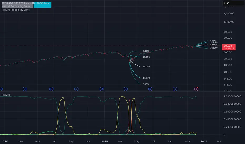
Hierarchical Hidden Markov Model - Probability Cone
The Hierarchical Hidden Markov Model - Probability Cone Indicator employs Hierarchical Hidden Markov Models for forecasting future price movements in financial markets. HHMMs are statistical tools that predict transitions between hidden states, such as different market regimes, based on observed data. This makes them valuable for understanding market behaviours and projecting future price trajectories. As discussed in the Hierarchical Hidden Markov Model indicator, HHMMs predict future states and their associated outputs based on the current state and model parameters. This tool is fundamentally very similar to the traditional HMM . The application of the HHMM for generating a probability cone forecast is therefore also fundamentally the same between HMM and HHMM. Despite their significant similarity I will go through the same fundamental examples of how probability cone is generated for the HHMM as I did for the HMM probability cone .
As you might know by now the probability cone indicator uses the knowledge about the current identified "state" or "regime" and with the help of transition probabilities, emission probabilities and initial probabilities generate a probabilistic forecast of the expected future price movements. To better understand the behind the Probability Cone we encourage you to use and learn about our free version of the Probability Cone as well as for even deeper understanding the Probability Cone Pro.
WHAT ARE REGIME DEPENDENT FORECASTS
We established that the indicator creates probabilistic forecasts of future price movements dependent on the current identified "state" or market "regime" via the Hidden Markov Model. In the image below we can see an example.
In this example we can see 4 different probability cones forecasting a 70% and 90% probability range (15% and 5% quantiles respectively). What you may notice is that the 4 probability cones look vastly different, despite using the same probability ranges as well as being generated from the same model trained on virtually the same data. What allows for this difference in the forecast, is conditioning the forecast on the current most likely identified state by the HHMM.
The first most cone is generating a forecast taking into account that the model identified the current market condition to be a extremely low in volatility this is a characteristic of the state identified by the light green coloured posterior probability. The second cone is significantly wider as well as has a negative drift, this is the case because that state identified by the red posterior probability is characterised by the most extreme volatility along with significant negative returns. The cone after that remains quite wide however is again associated with positive returns, this is characteristic of the state that the model identified via a high yelow coloured posterior probability. The last probability cone is again generated from a state that is characterised by quite low volatility albeit not the lowest. We can also see the state associated with that behaviour is identified by the high dark green posterior probability which is the highest at that time.
NOTE! Those are within sample forecasts, you can find more information on the difference between within sample model fit and out of sample prediction in the HHMM indicator description
This indicator also allows you to specify whether you wish to display probability based labels at the edges of the cone or whether you would prefer to display percent change based labels. With percent change labels you get the exact percentage value of the probabilistic increase or decrease of the price. See the example below
BARS BACK OFFSET vs DATE BASED OFFSET
The cones position can be offset by specifying the number of bars we wish to move it back similarly as with the rest of probability cone indicators. This indicator has however an additional, date based offset implemented. A user can therefore specify the position of the cone by specifying a date in the settings. The advantage of using the date based offset is that once it is turned on the user can also slide the cone up and down the chart with their mouse without having to manually adjust the date in the settings.
DIFFICULTIES WITH GENERATING FORECASTS (advanced):
The estimation of the probability cone, gets more difficult the more complex the model gets. A simple normal distribution probability cone can scale the distribution over time by simply multiplying the drift by the number of time steps and the volatility by the square root of time steps we wish to forecast for. More complex distributions often have to rely on mode advanced methods like convolutions, monte carlo or other kinds of approximations.
To estimate the probability cone forecast for the Hierarchial Hidden Markov Model, the indicator integrates two primary methodologies: Gaussian approximation and importance sampling. The Gaussian approximation is utilised for estimating the central 90% of future prices. This method provides a quick and efficient estimation within this central range, capturing the most likely price movements. The gaussian approximation will result in a forecast with an equal mean and variance as the true forecast, it will however not accurately reflect higher moments like skewness and kurtosis. For that reason the tail quantiles, which represent extreme price movements beyond the central range (90%), are estimated via importance sampling. This approach ensures a more accurate estimation of the skewness and kurtosis associated with extreme scenarios. While importance sampling leverages the flexibility of Monte Carlo as well as attempts to increase its efficiency by sampling from more precise areas of the distribution, the importance sampling may still underestimate most extreme quantiles associated with the lowest probabilities which is an inherent limitation of the indicator.
Example of gaussian approximation cone for probabilities above 5% (90% range):
Example of importance sampling cone for tail probabilities lower than 5% (beyond 90% range):
WARNING!
As per usual understand that the probabilities are estimations and best guesses based on the historical data and the patterns identified by the model and do not represent the true probability which is unknown in reality.
Settings:
- Source: Data source used for the model
- Forecast Period: Number of bars ahead for generating forecasts.
- Simulation Number: Number of Monte Carlo simulations to run in the case of importance sampling
-Body Probability: Specifies the inner range of the probability cone. The probability specifies the ammount of observations that are expected to fall outside of this range
- Tail Probability: Specifies the outter range of the probability cone. When this probability is under 5%, importance sampling will turn on
- Lock Cone: When ticked on, the cone will be locked at its current position.
- Offset Cone Based on Date: When ticked on, the position of the cone will be determined by the selected date.
- Offset: When "Offset Cone Based on Date" is turned off, you can use offset setting to specify the position of the cone projection.
- Date: When "Offset Cone Based on Date" is turned on, you can use the date setting to specify the date from which the forecast starts.
- Reestimate Model Every N Bars: This is especially useful if you wish to use the indicator on lower timeframes where model estimation might take longer than for the new datapoint to arrive. In that case you can specify after how many bars the model should be reestimated.
- Training Period: Length of historical data used to train the HMM.
- Expectation Maximization Iterations: Number of iterations for the EM algorithm.
- Cone Colors: Customizable colors for the probability cone, when approximation is on and when importance sampling is on
NY 8-11 Statistical Bias NQ 【Donkey】This indicator analyzes historical session patterns to predict directional bias during the NY 8:00-11:00 AM trading window for Micro NQ futures.
Simple Logic:
Monitors 3 sessions: Asian (20:00-02:00), London (02:00-08:00), NY (08:00-11:00)
Identifies current pattern based on: ranges, opening positions, and sweep behaviors
Searches database of 2.080 historical sessions for matching patterns
Displays statistical probability: "X% reached HIGH" vs "Y% reached LOW"
Shows expected drawdown levels for risk management
Example: If pattern shows "77% HIGH bias" → historically, 77 out of 100 similar sessions reached London high during NY 8-11 window.
Key Features
✅ Statistical Database:2.080 real sessions analyzed, 236 unique patterns
✅ 4-Level Pattern Matching: Finds best match with minimum 25 occurrences
✅ Live Bias Display: Shows HIGH% vs LOW% probability in real-time table
✅ Risk Management Zones: Visual drawdown levels (50%, 75%, 90%) + stop-loss suggestion
✅ No Repainting: Calculations made in real-time, no look-ahead bias
✅ Session Visualization: Color-coded boxes for Asian/London/NY ranges
How Pattern Matching Works
5 Components Analyzed:
Asian Range: Above/Below average
London Open: Above/Below Asian 50%
London Sweep: H, L, DH (double high→low), DL (double low→high), N (none)
London Range: Above/Below average
NY Open: Above/Below London 50%
Cascade Search (finds best available match):
Level 1: All 5 components (most specific)
Level 2: 4 components (drops London Range)
Level 3: 3 components (core pattern)
Level 4: 2 components (minimal pattern)
Validity: Only displays patterns with ≥25 historical occurrences.
Interpretation
Bias Table Shows:
Pattern match level (1-4) and historical count
Session characteristics (ranges, sweeps, positions)
TOTAL HIGH % = probability of reaching London high
TOTAL LOW % = probability of reaching London low
Bias strength: ⭐⭐⭐ STRONG (≥70%), ⭐⭐ MEDIUM (60-69%), ⭐ WEAK (<60%)
Drawdown Zones (for winning trades):
🟢 Green: 50% of winners stayed within this level
🟡 Yellow: 75% of winners stayed within this level
🟠 Orange: 90% of winners stayed within this level
🔴 Red Line: Suggested stop-loss (95th percentile + buffer)
Settings
Fully Customizable:
Timezone selection (auto-detects sessions correctly)
Minimum session threshold (default: 25)
Toggle boxes, lines, labels, drawdown zones
Complete color customization
Table size and position
Best Use Cases
✅ Optimal Setup:
Instrument: Micro NQ (MNQ) futures
Timeframe: Only 1-minute
Timezone: America/New_York
Historical data: 8+ years loaded
✅ Trading Approach:
Wait for pattern confirmation (≥25 sessions)
Prefer STRONG bias (≥70%) for higher confidence
Use drawdown zones for stop placement
Combine with price action confirmation
Avoid major news events (FOMC, NFP)
⚠️ Required Disclaimers
IMPORTANT RISK WARNINGS:
Past Performance ≠ Future Results: Historical statistics do NOT guarantee future outcomes
Not Financial Advice: Educational tool for statistical analysis only
Risk of Loss: Futures trading involves substantial risk of loss
No Guarantees: Individual trades WILL result in losses regardless of percentages shown
Requires Knowledge: Best for traders familiar with session analysis and risk management
Instrument-Specific: Optimized for Micro NQ - test before using elsewhere
Never risk more than you can afford to lose. Always use proper risk management.

Hidden Markov Model - Probability Cone
The Hidden Markov Model - Probability Cone Indicator employs Hidden Markov Models (HMMs) for forecasting future price movements in financial markets. HMMs are statistical tools that predict transitions between hidden states, such as different market regimes, based on observed data. This makes them valuable for understanding market behaviours and projecting future price trajectories. As discussed in the Hidden Markov Model indicator, HMMs predict future states and their associated outputs based on the current state and model parameters.
The probability cone indicator therefore uses the knowledge about the current identified "state" or "regime" and with the help of transition probabilities, emission probabilities and initial probabilities generate a probabilistic forecast of the expected future price movements. To better understand the behind the Probability Cone we encourage you to use and learn about our free version of the Probability Cone as well as for even deeper understanding the Probability Cone Pro.
WHAT ARE REGIME DEPENDENT FORECASTS
As mentioned above the indicator creates probabilistic forecasts of future price movements dependent on the current identified "state" or market "regime" via the Hidden Markov Model. In the image below we can see an example.
In this example we can see 3 different probability cones forecasting a 70% and 90% probability range (15% and 5% quantiles respectively). What you may notice is that the 3 probability cones look vastly different, despite using the same probability ranges as well as being generated from the same model trained on virtually the same data. What allows for this difference in the forecast is conditioning the forecast on the current most likely identified state by the HMM.
The first most wide cone is generating a forecast taking into account that the model identified the current market condition to be a very volatile which is a characteristic of the state identified by the orange coloured posterior probability. The second cone is significantly more narrow as that state identified by the purple posterior probability is characterised by lower volatility. Nevertheless, the last probability cone is generated from the state that is characterised by the lowest volatility, we can also see the light blue posterior probability to be the highest at that time.
The indicator also allows you to specify whether you wish to display probability based labels at the edges of the cone or whether you would prefer to display percent change based labels. With percent change labels you get the exact percentage value of the probabilistic increase or decrease of the price. See the example below
BARS BACK OFFSET vs DATE BASED OFFSET
The cones position can be offset by specifying the number of bars we wish to move it back similarly as with the rest of probability cone indicators. This indicator has however an additional, date based offset implemented. A user can therefore specify the position of the cone by specifying a date in the settings. The advantage of using the date based offset is that once it is turned on the user can also slide the cone up and down the chart with their mouse without having to manually adjust the date in the settings.
DIFFICULTIES WITH GENERATING FORECASTS (advanced):
The estimation of the probability cone, gets more difficult the more complex the model gets. A simple normal distribution probability cone can scale the distribution over time by simply multiplying the drift by the number of time steps and the volatility by the square root of time steps we wish to forecast for. More complex distributions often have to rely on mode advanced methods like convolutions, monte carlo or other kinds of approximations.
To estimate the probability cone forecast for the Hidden Markov Model, the indicator integrates two primary methodologies: Gaussian approximation and importance sampling. The Gaussian approximation is utilized for estimating the central 90% of future prices. This method provides a quick and efficient estimation within this central range, capturing the most likely price movements. The gaussian approximation will result in a forecast with an equal mean and variance as the true forecast, it will however not accurately reflect higher moments like skewness and kurtosis. For that reason the tail quantiles, which represent extreme price movements beyond the central range (90%), are estimated via importance sampling. This approach ensures a more accurate estimation of the skewness and kurtosis associated with extreme scenarios. While impoortance sampling leverages the flexibility of monte carlo as well as attempts to increase its efficiency by sampling from more precise areas of the distribution, the importance sampling may still underestimate most extreme quantiles associated with the lowest probabilties which is an inherent limitation of the indicator.
Example of gaussian approximation cone for probabilities above 5% (90% range):
Example of importance sampling cone for tail probabilities lower than 5% (beyond 90% range):
WARNING!
As per usual understand that the probabilities are estimations and best guesses based on the historical data and the patterns identified by the model and do not represent the true probability which is unknown in reality.
Settings:
- Source: Data source used for the model
- Forecast Period: Number of bars ahead for generating forecasts.
- Simulation Number: Number of Monte Carlo simulations to run in the case of importance sampling
-Body Probability: Specifies the inner range of the probability cone. The probability specifies the ammount of observations that are expected to fall outside of this range
- Tail Probability: Specifies the outter range of the probability cone. When this probability is under 5%, importance sampling will turn on
- Lock Cone: When ticked on, the cone will be locked at its current position.
- Offset Cone Based on Date: When ticked on, the position of the cone will be determined by the selected date.
- Offset: When "Offset Cone Based on Date" is turned off, you can use offset setting to specify the position of the cone projection.
- Date: When "Offset Cone Based on Date" is turned on, you can use the date setting to specify the date from which the forecast starts.
- Reestimate Model Every N Bars: This is especially useful if you wish to use the indicator on lower timeframes where model estimation might take longer than for the new datapoint to arrive. In that case you can specify after how many bars the model should be reestimated.
- Training Period: Length of historical data used to train the HMM.
- Expectation Maximization Iterations: Number of iterations for the EM algorithm.
- Cone Colors: Customizable colors for the probability cone, when approximation is on and when importance sampling is on

Watermark | Bar Time | Average Daily RangeMulti Info Panel & Watermark
Multi Info Panel & Watermark is a utility indicator that displays several pieces of chart information in a single, customizable panel. It is designed to support intraday and swing analysis by making key data—such as symbol details, date, and average daily range—easy to see at a glance, as well as providing simple tools for notes and backtesting.
Features
Watermark / Custom Note
Optional text overlay that can be used as a watermark or personal note.
Can display a strategy name, reminder, or any other user-defined label on the chart.
Ticker Info
Shows information about the currently active symbol on the chart (for example, symbol name and other basic details depending on the inputs).
Helps keep track of which market or pair is being analyzed, especially when using multiple charts.
Current Date
Displays the current date directly on the chart.
Useful for screenshots, journaling, and documenting analysis.
Average Daily Range (ADR)
Calculates the average daily range of the active symbol over a user-defined number of recent days.
Helps visualize how much price typically moves in a day, which can support position sizing, target setting, or volatility awareness within your own trading approach.
Open Bar Time Marker
Marks the open time of a selected bar (for example, a session open or a specific reference bar).
Primarily intended as a visual aid for manual backtesting and reviewing historical price action.
Usage
Use the watermark and ticker info to keep your charts labeled and organized.
Refer to the ADR readout to understand typical daily volatility of the instrument you are studying.
Use the date and open bar time marker when creating screenshots, trade journals, or when replaying historical sessions for review.
This script does not generate trading signals and does not guarantee any performance or results. It is provided solely as an informational and visualization tool. Always combine it with your own analysis, risk management, and decision-making. Nothing in this indicator or description should be considered financial advice.

Probability Cone ProProbability Cone Pro is based on the Expected Move Pro . While Expected Move only shows the historical value band on every bar, probability cone extend the period in the future and plot a cone or curve shape of the probable range. It plots the range from bar 1 all the way to any specified number of bars up to 1000.
Probability Cone Pro is an upgraded version of the Probability Cone indicator that uses a Normal Distribution to model the returns. This newer version uses a maximum likelihood estimation for Asymmetric Laplace distribution parameters. Asymmetric Laplace distribution takes into account fatter tails and volatility clustering during low volatility. So it will be thinner in the body (eg: <70% range) and fatter in the tails (>95% range) which fits the stock return better. Despite a better fit users should not blindly follow the probabilities derived from the indicator and should understand that these are very precise estimations of probability based on historical data, not the true probability which is in reality unknown.
When we compare the more peaked asymmetric laplace to the bell curve shaped normal distribution we can see that the asymmetric laplace fits the empirical data (blue histogram) significantly better. The fit is improved in both the body (middle peaked part) as well as in the fatter tails (more of extreme occurrences far from the center)
The area of probability range is based on an inverse cumulative distribution function. The inverse cumulative distribution gives the range of price for given input probability. People can adjust the range by adjusting the input probability in the settings. The entered probability will be shown at the edges of the cone when the “show probability” setting is on.
The indicator allows for specifying the probability for 2 quantiles on each side of the distribution , therefore 4 distinct probability values. The exact probability input is another distinction compared to the Normal Distribution based Probability Cone, in which the probability range is determined by the input of a standard deviation. Additionally now the displayed labels at the edges of the probability cone no longer correspond to the total number of outcomes that are expected to occur within the specific range, instead we chose to display the inverse which is the probability of outcomes outside of the specified range. See comparison below:
Probability cone pro with 68% and 95% ranges also defined by 16% and 2.5% probabilities at the tails on both sides:
Normal Probability cone with 68% and 95% ranges defined by 1st and 2nd standard deviation
SETTINGS:
Bars Back : Number of bars the cone is offset by.
Forecast Bar: Number of bars we forecast the cone for in the future.
Lock Cone : Specify whether we wish t lock the cone to the current bar, so it does not move when new bars arrive.
Show Probability : Specify whether you wish to show the probability labels at the edges of the cone.
Source : Source for computation of log returns whose distribution we forecast
Drift : Whether to take into account the drift in returns or assume 0 mean for the distribution.
Period: The sampling period or lookback for both the drift and the volatility estimation (full distribution estimation).
Up/Down Probabilities: 4 distinct probabilities are specified, 2 for the upper and 2 for the lower side of the distribution.

Expected Move ProExpected Move is the amount that an asset is predicted to increase or decrease from its current price, based on the current levels of volatility.
This Expected Move Pro indicator uses a maximum likelihood estimation for Asymmetric Laplace distribution parameters, and is an upgrade from the regular Expected Move indicator that uses a Normal Distribution. The use of the Asymmetric Laplace distribution ensures a probability range more accurate than the more common expected moves based on a normal distribution assumption for returns. Asymmetric Laplace distribution takes in account fatter tails and volatility clustering during low volatility. So it will be thinner in the body (eg: <70% range) and fatter in the tails (>95% range) which fits the stock return better.
When we compare the more peaked asymmetric laplace to the bell curve shaped normal distribution we can see that the asymmetric laplace fits the empirical data (blue histogram) significantly better. The fit is improved in both the body (middle peaked part) as well as in the fatter tails (more of extreme occurrences far from the center)
EXPECTED MOVE PROBABILITY:
In the expected move settings, the user can specify the range probability they wish to display. In a normal distribution a 1 standard deviation range corresponds to a range within which just under 70% of observations fall. So to specify a 70% probability range one would set 15% probability for both the upper and lower range.
For the more extreme ranges a two tail function is used so the user can only specify one probability. When 5% probability is specified the range will cover 95% and on each side of the range the probability of an occurence that extreme will be 2.5%. In the above Image we can see two tail probabilities specified at 5% and 1%, covering the 95% and 99% ranges respectively.
The indicator also allows for multi timeframe usecases. One can request a daily or perhaps even weekly expected move on an hourly chart, like we see below.
SETTINGS:
Resolution: Specify the timeframe and if you want to use the multi timeframe functionality.
Real Time : Do you wish the expected move to adjust with the current open price or do you wish it to be a forecast based on the yesterdays close. If latter, keep it OFF.
Sample Size : Lookback or the number of bars we sample in the calculation.
Optimization : Keep it on for speed purposes, only slightly higher precision will be achieved without optimization.
Probabilities: One tail - left and right, specify probability for each side of the range, two tail - single probability split in half for each side of the range
Center : Displays the central line which is the central tendency of a distribution / the median
Hide History : Hides expected moves and only the expected move for the current bar remains.
Plot Style Settings : One can adjust the line styles, box styles as well as width and transparency.

Probability Cone█ Overview:
Probability Cone is based on the Expected Move . While Expected Move only shows the historical value band on every bar, probability panel extend the period in the future and plot a cone or curve shape of the probable range. It plots the range from bar 1 all the way to bar 31.
In this model, we assume asset price follows a log-normal distribution and the log return follows a normal distribution.
Note: Normal distribution is just an assumption; it's not the real distribution of return.
The area of probability range is based on an inverse normal cumulative distribution function. The inverse cumulative distribution gives the range of price for given input probability. People can adjust the range by adjusting the standard deviation in the settings. The probability of the entered standard deviation will be shown at the edges of the probability cone.
The shown 68% and 95% probabilities correspond to the full range between the two blue lines of the cone (68%) and the two purple lines of the cone (95%). The probabilities suggest the % of outcomes or data that are expected to lie within this range. It does not suggest the probability of reaching those price levels.
Note: All these probabilities are based on the normal distribution assumption for returns. It's the estimated probability, not the actual probability.
█ Volatility Models :
Sample SD : traditional sample standard deviation, most commonly used, use (n-1) period to adjust the bias
Parkinson : Uses High/ Low to estimate volatility, assumes continuous no gap, zero mean no drift, 5 times more efficient than Close to Close
Garman Klass : Uses OHLC volatility, zero drift, no jumps, about 7 times more efficient
Yangzhang Garman Klass Extension : Added jump calculation in Garman Klass, has the same value as Garman Klass on markets with no gaps.
about 8 x efficient
Rogers : Uses OHLC, Assume non-zero mean volatility, handles drift, does not handle jump 8 x efficient.
EWMA : Exponentially Weighted Volatility. Weight recently volatility more, more reactive volatility better in taking account of volatility autocorrelation and cluster.
YangZhang : Uses OHLC, combines Rogers and Garmand Klass, handles both drift and jump, 14 times efficient, alpha is the constant to weight rogers volatility to minimize variance.
Median absolute deviation : It's a more direct way of measuring volatility. It measures volatility without using Standard deviation. The MAD used here is adjusted to be an unbiased estimator.
You can learn more about each of the volatility models in out Historical Volatility Estimators indicator.
█ How to use
Volatility Period is the sample size for variance estimation. A longer period makes the estimation range more stable less reactive to recent price. Distribution is more significant on larger sample size. A short period makes the range more responsive to recent price. Might be better for high volatility clusters.
People usually assume the mean of returns to be zero. To be more accurate, we can consider the drift in price from calculating the geometric mean of returns. Drift happens in the long run, so short lookback periods are not recommended.
The shape of the cone will be skewed and have a directional bias when the length of mean is short. It might be more adaptive to the current price or trend, but more accurate estimation should use a longer period for the mean.
Using a short look back for mean will make the cone having a directional bias.
When we are estimating the future range for time > 1, we typically assume constant volatility and the returns to be independent and identically distributed. We scale the volatility in term of time to get future range. However, when there's autocorrelation in returns( when returns are not independent), the assumption fails to take account of this effect. Volatility scaled with autocorrelation is required when returns are not iid. We use an AR(1) model to scale the first-order autocorrelation to adjust the effect. Returns typically don't have significant autocorrelation. Adjustment for autocorrelation is not usually needed. A long length is recommended in Autocorrelation calculation.
Note: The significance of autocorrelation can be checked on an ACF indicator.
ACF
Time back settings shift the estimation period back by the input number. It's the origin of when the probability cone start to estimation it's range.
E.g., When time back = 5, the probability cone start its prediction interval estimation from 5 bars ago. So for time back = 5 , it estimates the probability range from 5 bars ago to X number of bars in the future, specified by the Forecast Period (max 1000).
█ Warnings:
People should not blindly trust the probability. They should be aware of the risk evolves by using the normal distribution assumption. The real return has skewness and high kurtosis. While skewness is not very significant, the high kurtosis should be noticed. The Real returns have much fatter tails than the normal distribution, which also makes the peak higher. This property makes the tail ranges such as range more than 2SD highly underestimate the actual range and the body such as 1 SD slightly overestimate the actual range. For ranges more than 2SD, people shouldn't trust them. They should beware of extreme events in the tails.
The uncertainty in future bars makes the range wider. The overestimate effect of the body is partly neutralized when it's extended to future bars. We encourage people who use this indicator to further investigate the Historical Volatility Estimators , Fast Autocorrelation Estimator , Expected Move and especially the Linear Moments Indicator .
The probability is only for the closing price, not wicks. It only estimates the probability of the price closing at this level, not in between.

EMA + Sessions + RSI Strategy v1.0A professional trading strategy that combines multiple technical indicators for high-probability entries. This system uses EMA crossovers, RSI zone filtering, and trend confirmation to identify optimal trading opportunities while managing risk with advanced position management tools.
Key Features:
✅ Dual Entry Signals (EMA21 + EMA100 crossover conditions)
✅ Trend Filter EMA750 (trade only with the major trend)
✅ Complete Risk Management (SL 1%, TP 3% default)
✅ Trailing Stop & Breakeven (maximize profits, protect capital)
✅ Compact Statistics Table (real-time performance metrics)
✅ RSI & Session Filters (avoid low-probability setups)
✅ Optional Pyramiding (scale into winning positions)
Perfect for swing trading and trend-following on any timeframe. Fully customizable to match your trading style.

Position Size Calculator + Live R/R Panel — SMC/ICT (@PueblaATH)Position Size + Live R/R Panel — SMC/ICT (@PueblaATH)
Position Size + Live R/R Panel — SMC/ICT (@PueblaATH) is a professional-grade risk management and execution module built for Smart Money Concepts (SMC) and ICT Traders who require accurate, repeatable, institution-style trade planning.
This tool delivers precise position sizing, R:R modeling, leverage and margin projections, fee-adjusted PnL outcomes, and real-time execution metrics—all directly on the chart. Optimized for crypto, forex, and futures, it provides scalpers, day traders, and swing traders with the clarity needed to execute high-quality trades with confidence and consistency.
What the Indicator Does
Institutional Position Sizing Engine
Calculates position size based on account balance, % risk, and SL distance.
Supports custom minimum lot size rounding across crypto, FX, indices, and derivatives.
Intelligent direction logic (Auto / Long / Short) based on SMC/ICT structure.
Advanced Risk/Reward & Profit Modeling
Real-time R:R ratio using actual rounded position size.
Live PnL readout that updates with price movements.
Gross & net profit projections with full fee deduction.
Execution Planning with Draggable Levels
Entry, SL, and TP levels fully draggable for fast scenario modeling.
Automatic projected lines backward/forward with clean label alignment.
TP and SL tags include % movement from Entry, ideal for SMC/ICT journaling.
Precise modeling of real exchange fee structures
Maker fee per side
Taker fee per side
Mixed fee modes (Maker entry, Taker exit, Average, etc.)
Leverage & Margin Forecasting
Margin requirements displayed for 3 customizable leverage settings.
Helps traders understand capital commitment before executing the trade.
Useful for futures, crypto perps, and CFD setups.
Clean HUD Panel for Rapid Decision-Making
A full professional trading panel displays:
Target & actual risk
Position size
Entry / SL / TP
TP/SL percentage distance
Gross profit
Net profit (after fees)
Fees @ TP and @ SL
Live PnL
Margin requirements
Optimized for SMC & ICT Workflows
Perfect for traders using:
Breakers, FVGs, OBs
Liquidity sweeps
Session models
Precision entries (OTE, Displacement, Rebalancing)
Leverage-based execution (crypto perps, futures)
How to Use It
Attach the indicator to your chart.
Set account balance, risk %, fee model, and leverage presets.
Drag Entry, SL, and TP to shape the setup.
View instant calculations of: Position size; R:R; Net PnL after fees; Margin required
Use it as your pre-trade checklist & execution model.
Originality & Credits
This script is an original creation by @PueblaATH, released under the MPL 2.0 license.
It does not copy, modify, or repackage any existing TradingView code.
All logic—including the fee engine, margin calculator, responsive HUD, dynamic risk model, and visual execution system—is authored specifically for this indicator.


