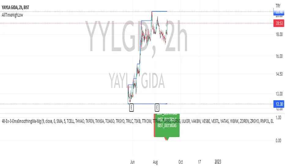
AllTimeHighLowLibrary "AllTimeHighLow"
Provides functions calculating the all-time high/low of values.
hi(val)
Calculates the all-time high of a series.
Parameters:
val : Series to use (`high` is used if no argument is supplied).
Returns: The all-time high for the series.
lo(val)
Calculates the all-time low of a series.
Parameters:
val : Series to use (`low` is used if no argument is supplied).
Returns: The all-time low for the series.
Statistics
L_BetaLibrary "L_Beta"
TODO: add library description here
length()
beta()
simple_beta()
index_selector()

CalulateWinLossLibrary "CalulateWinLoss"
TODO: add library description here
colorwhitered(x)
TODO: add function description here
Parameters:
x : TODO: add parameter x description here
Returns: TODO: add what function returns
colorredwhite()
cal()

FunctionPatternFrequencyLibrary "FunctionPatternFrequency"
Counts the word or integer number pattern frequency on a array.
reference:
rosettacode.org
count(pattern)
counts the number a pattern is repeated.
Parameters:
pattern : : array : array with patterns to be counted.
Returns:
array : list of unique patterns.
array : list of counters per pattern.
usage:
count(array.from('a','b','c','a','b','a'))
count(pattern)
counts the number a pattern is repeated.
Parameters:
pattern : : array : array with patterns to be counted.
Returns:
array : list of unique patterns.
array : list of counters per pattern.
usage:
count(array.from(1,2,3,1,2,1))

DatasetWeatherTokyoMeanAirTemperatureLibrary "DatasetWeatherTokyoMeanAirTemperature"
Provides a data set of the monthly mean air temperature (°C) for the city of Tokyo in Japan.
this was just for fun, no financial implications in this.
reference:
www.data.jma.go.jp
TOKYO WMO Station ID:47662 Lat 35o41.5'N Lon 139o45.0'E
year_()
the years of the data set.
Returns: array : year values.
january()
the january values of the dataset
Returns: array\ : data values for january.
february()
the february values of the dataset
Returns: array\ : data values for february.
march()
the march values of the dataset
Returns: array\ : data values for march.
april()
the april values of the dataset
Returns: array\ : data values for april.
may()
the may values of the dataset
Returns: array\ : data values for may.
june()
the june values of the dataset
Returns: array\ : data values for june.
july()
the july values of the dataset
Returns: array\ : data values for july.
august()
the august values of the dataset
Returns: array\ : data values for august.
september()
the september values of the dataset
Returns: array\ : data values for september.
october()
the october values of the dataset
Returns: array\ : data values for october.
november()
the november values of the dataset
Returns: array\ : data values for november.
december()
the december values of the dataset
Returns: array\ : data values for december.
annual()
the annual values of the dataset
Returns: array\ : data values for annual.
select_month(idx)
get the temperature values for a specific month.
Parameters:
idx : int, month index (1 -> 12 | any other value returns annual average values).
Returns: array\ : data values for selected month.
select_value(year_, month_)
get the temperature value of a specified year and month.
Parameters:
year_ : int, year value.
month_ : int, month index (1 -> 12 | any other value returns annual average values).
Returns: float : value of specified year and month.
diff_to_median(month_)
the difference of the month air temperature (ºC) to the median of the sample.
Parameters:
month_ : int, month index (1 -> 12 | any other value returns annual average values).
Returns: float : difference of current month to median in (Cº)

FunctionDynamicTimeWarpingLibrary "FunctionDynamicTimeWarping"
"In time series analysis, dynamic time warping (DTW) is an algorithm for
measuring similarity between two temporal sequences, which may vary in
speed. For instance, similarities in walking could be detected using DTW,
even if one person was walking faster than the other, or if there were
accelerations and decelerations during the course of an observation.
DTW has been applied to temporal sequences of video, audio, and graphics
data — indeed, any data that can be turned into a linear sequence can be
analyzed with DTW. A well-known application has been automatic speech
recognition, to cope with different speaking speeds. Other applications
include speaker recognition and online signature recognition.
It can also be used in partial shape matching applications."
"Dynamic time warping is used in finance and econometrics to assess the
quality of the prediction versus real-world data."
~~ wikipedia
reference:
en.wikipedia.org
towardsdatascience.com
github.com
cost_matrix(a, b, w)
Dynamic Time Warping procedure.
Parameters:
a : array, data series.
b : array, data series.
w : int , minimum window size.
Returns: matrix optimum match matrix.
traceback(M)
perform a backtrace on the cost matrix and retrieve optimal paths and cost between arrays.
Parameters:
M : matrix, cost matrix.
Returns: tuple:
array aligned 1st array of indices.
array aligned 2nd array of indices.
float final cost.
reference:
github.com
report(a, b, w)
report ordered arrays, cost and cost matrix.
Parameters:
a : array, data series.
b : array, data series.
w : int , minimum window size.
Returns: string report.

FunctionKellyCriterionLibrary "FunctionKellyCriterion"
Kelly criterion methods.
the kelly criterion helps with the decision of how much one should invest in
a asset as long as you know the odds and expected return of said asset.
simplified(win_p, rr)
simplified version of the kelly criterion formula.
Parameters:
win_p : float, probability of winning.
rr : float, reward to risk rate.
Returns: float, optimal fraction to risk.
usage:
simplified(0.55, 1.0)
partial(win_p, loss_p, win_rr, loss_rr)
general form of the kelly criterion formula.
Parameters:
win_p : float, probability of the investment returns a positive outcome.
loss_p : float, probability of the investment returns a negative outcome.
win_rr : float, reward on a positive outcome.
loss_rr : float, reward on a negative outcome.
Returns: float, optimal fraction to risk.
usage:
partial(0.6, 0.4, 0.6, 0.1)
from_returns(returns)
Calculate the fraction to invest from a array of returns.
Parameters:
returns : array trade/asset/strategy returns.
Returns: float, optimal fraction to risk.
usage:
from_returns(array.from(0.1,0.2,0.1,-0.1,-0.05,0.05))
final_f(fraction, max_expected_loss)
Final fraction, eg. if fraction is 0.2 and expected max loss is 10%
then you should size your position as 0.2/0.1=2 (leverage, 200% position size).
Parameters:
fraction : float, aproximate percent fraction invested.
max_expected_loss : float, maximum expected percent on a loss (ex 10% = 0.1).
Returns: float, final fraction to invest.
usage:
final_f(0.2, 0.5)
hpr(fraction, trade, biggest_loss)
Holding Period Return function
Parameters:
fraction : float, aproximate percent fraction invested.
trade : float, profit or loss in a trade.
biggest_loss : float, value of the biggest loss on record.
Returns: float, multiplier of effect on equity so that a win of 5% is 1.05 and loss of 5% is 0.95.
usage:
hpr(fraction=0.05, trade=0.1, biggest_loss=-0.2)
twr(returns, rr, eps)
Terminal Wealth Relative, returns a multiplier that can be applied
to the initial capital that leadds to the final balance.
Parameters:
returns : array, list of trade returns.
rr : float , reward to risk rate.
eps : float , minimum resolution to void zero division.
Returns: float, optimal fraction to invest.
usage:
twr(returns=array.from(0.1,-0.2,0.3), rr=0.6)
ghpr(returns, rr, eps)
Geometric mean Holding Period Return, represents the average multiple made on the stake.
Parameters:
returns : array, list of trade returns.
rr : float , reward to risk rate.
eps : float , minimum resolution to void zero division.
Returns: float, multiplier of effect on equity so that a win of 5% is 1.05 and loss of 5% is 0.95.
usage:
ghpr(returns=array.from(0.1,-0.2,0.3), rr=0.6)
run_coin_simulation(fraction, initial_capital, n_series, n_periods)
run multiple coin flipping (binary outcome) simulations.
Parameters:
fraction : float, fraction of capital to bet.
initial_capital : float, capital at the start of simulation.
n_series : int , number of simulation series.
n_periods : int , number of periods in each simulation series.
Returns: matrix(n_series, n_periods), matrix with simulation results per row.
usage:
run_coin_simulation(fraction=0.1)
run_asset_simulation(returns, fraction, initial_capital)
run a simulation over provided returns.
Parameters:
returns : array, trade, asset or strategy percent returns.
fraction : float , fraction of capital to bet.
initial_capital : float , capital at the start of simulation.
Returns: array, array with simulation results.
usage:
run_asset_simulation(returns=array.from(0.1,-0.2,0.-3,0.4), fraction=0.1)
strategy_win_probability()
calculate strategy() current probability of positive outcome in a trade.
strategy_avg_won()
calculate strategy() current average won on a trade with positive outcome.
strategy_avg_loss()
calculate strategy() current average lost on a trade with negative outcome.

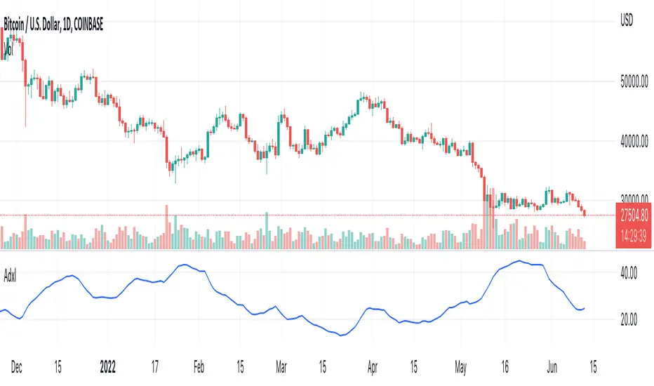
AdxlLibrary "Adxl"
Functions to calculate the Average Directional Index
getDirectionUp(bar, lookback)
Bar high changed from open for bar
Parameters:
bar : series int The bar to calculate at
lookback : series int The lookback period
Returns: series float
getDirectionDown(bar, lookback)
Bar low changed from open for bar
Parameters:
bar : series int The bar to calculate at
lookback : series int The lookback period
Returns: series float
getPositiveDirectionalMovement(bar, lookback)
Positive directional movement for bar during lookback
Parameters:
bar : series int The bar to calculate at
lookback : series int The lookback period
Returns: series float
getNegativeDirectionalMovement(bar, lookback)
Negative directional movement for bar during lookback
Parameters:
bar : series int The bar to calculate at
lookback : series int The lookback period
Returns: series float
getTrueRangeMovingAverage(bar, lookback)
True range moving average for bar during lookback
Parameters:
bar : series int The bar to calculate at
lookback : simple int The lookback period
Returns: series int
getDirectionUpIndex(bar, lookback)
Direction up index for bar during lookback
Parameters:
bar : series int The bar to calculate at
lookback : simple int The lookback period
Returns: series int
getDirectionDownIndex(bar, lookback)
Direction down index for bar during lookback
Parameters:
bar : series int The bar to calculate at
lookback : simple int The lookback period
Returns: series int
getTotalDirectionIndex(bar, lookback)
Total direction index for bar during lookback
Parameters:
bar : series int The bar to calculate at
lookback : simple int The lookback period
Returns: series int
getAverageDirectionalIndex(bar, lookback)
Average Directional Index (ADX) for bar during lookback
Parameters:
bar : series int The bar to calculate at
lookback : simple int The lookback period
Returns: series int
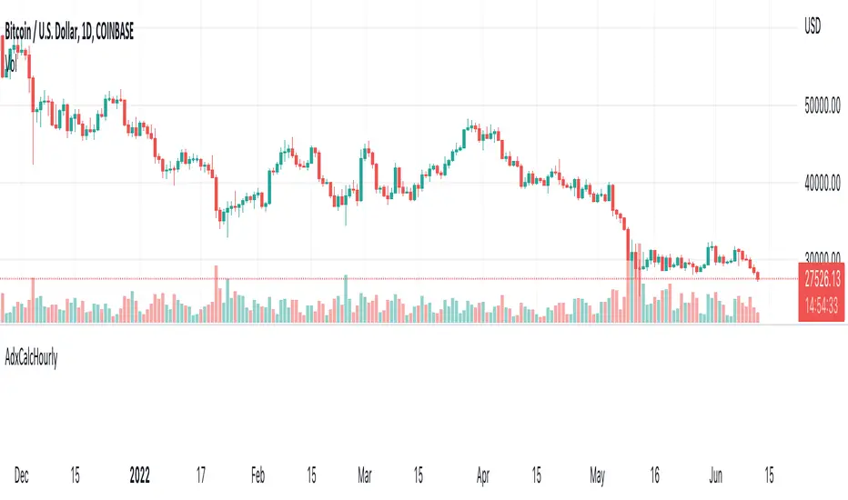
AdxCalcHourlyLibrary "AdxCalcHourly"
getBars()
getBars: Returns the number of bars to use in the historical lookback period
Returns: simple int
directionDown()
directionDown: Calculates the direction down for bar_index
Returns: series float
directionUp()
directionUp: Calculates the direction up for bar_index
Returns: series float
trueRangeMovingAverage()
trueRangeMovingAverage: Calculates the true range moving average over the historical lookback period
Returns: series float
positiveDirectionalMovement()
positiveDirectionalMovement: Calculates the positive direction movement for bar_index
Returns: series float
negativeDirectionalMovement()
negativeDirectionalMovement: Calculates the begative direction movement for bar_index
Returns: series float
totalDirectionDown()
totalDirectionDown: Calculates the total direction down for the historical lookback period
Returns: series float
totalDirectionUp()
totalDirectionUp: Calculates the total direction up for the historical lookback period
Returns: series float
totalDirection()
totalDirection: Calculates the total direction movement for the historical lookback period
Returns: series float
averageDirectionalIndex()
averageDirectionalIndex: Calculates the average directional index (ADX) based on the trend for the historical lookback period
Returns: series float
getAdxHistoricalAverage()
getAdxHistoricalAverage: Calculates the average directional index (ADX) for the historical lookback period
Returns: series float
getAdxHistoricalHigh()
getAdxHistoricalHigh: Calculates the historical high of the directional index (ADX) for the historical lookback period
Returns: series float
getAdxHistoricalLow()
getAdxHistoricalLow: Calculates the historical low of the directional index (ADX) for the historical lookback period
Returns: series float
getAdxOpinion()
getAdxOpinion: Calculatesa recomendation for the directional index (ADX) based on the historical lookback period
Returns: series float
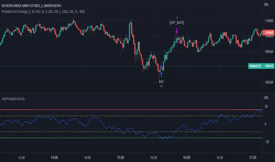
WpProbabilisticLibLibrary "WpProbabilisticLib"
Library that contains functions to calculate probabilistic based on historical candle analysis
CandleType(open, close) This function check what type of candle is, based on its close and open prices
Parameters:
open : series float (open price)
close : series float (close price)
Returns: This function return the candle type (1 for Bullish, -1 Bearish, 0 as Doji candle)
CandleTypePercentDiff(open, close, qtd_candles_before, consider_dojis) This function calculates the percentage difference between Bullish and Bearish in a candlestick range back in time and which is the type with the least occurrences
Parameters:
open : series float (open price series)
close : series float (close price series)
qtd_candles_before : simple int (Number of candles before to calculate)
consider_dojis : simple string (How to consider dojis (no consider "NO", as bearish "AS_RED", as bullish "AS_GREEN"))
Returns: tuple(float, int) (Returns the percentage difference between Bullish and Bearish candles and which type of candle has the least occurrences)
PivotThis library was designed to create three different datasets using Bill Williams fractals. The goal is to spot trends in reversal data and ultimately use these datasets to help predict future price reversals.
First, the pivot() function is used to initialize and populate three separate arrays (high pivot , low pivot , all pivots ). Since each high/low price depends on the bar_index, the bar_index, pivot direction(high/low), and high/low values are compressed into a string to maintain the data's integrity ("__"). Once each string array is populated and organized by bar_index, all three are returned inside a tuple. The return value must be deconstructed H,L,A =pivot() for each array's values to be accessed using getPivot() . This boilerplate allows for data to be accessed more efficiently in a recursive environment. getPivot() was designed to be used inside of a for or while block to populate matrices for further analyses. Again, getPivot() return values must be exposed through deconstruction. x,d,y =getPivot(). See code for more details.
pivot(int XLR) initializes and populates arrays
Parameters
XLR - number of bars to the left and right that must be lower for a high to be considered a pivotHigh, or vice versa. This number will drastically change the size and scope of the returned datasets. smaller values will produce much larger datasets, which might model short term price activity well. In contrast, larger values will produce smaller datasets which might model longer term price activity well.
Returns - tuple [string ]
getPivot(string arrayID, int index) accesses array data
Parameters
arrayID - the variable name for one of the three arrays returned by pivot().
index - the index of the provided array, with 0 being the most recent pivot point. can be set to " i " in a loop to access values recursively
Returns - tuple

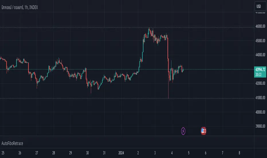
AutoFiboRetraceLibrary "AutoFiboRetrace"
TODO: add library description here
fun(x) TODO: add function description here
Parameters:
x : TODO: add parameter x description here
Returns: TODO: add what function returns
MonthlyReturnsVsMarketLibrary "MonthlyReturnsVsMarket" is a repackaging of the script here
Credits to @QuantNomad for orginal script
Now you can avoid to pollute your own strategy's code with the monthly returns table code and just import the library and call displayMonthlyPnL(int precision) function
To be used in strategy scripts.

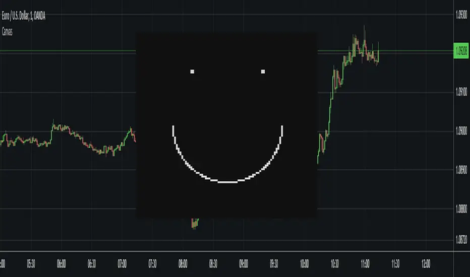
CanvasLibrary "Canvas"
A library implementing a kind of "canvas" using a table where each pixel is represented by a table cell and the pixel color by the background color of each cell.
To use the library, you need to create a color matrix (represented as an array) and a canvas table.
The canvas table is the container of the canvas, and the color matrix determines what color each pixel in the canvas should have.
max_canvas_size() Function that returns the maximum size of the canvas (100). The canvas is always square, so the size is equal to rows (as opposed to not rows multiplied by columns).
Returns: The maximum size of the canvas (100).
get_bg_color(color_matrix) Get the current background color of the color matrix. This is the default color used when erasing pixels or clearing a canvas.
Parameters:
color_matrix : The color matrix.
Returns: The current background color.
get_fg_color(color_matrix) Get the current foreground color of the color matrix. This is the default color used when drawing pixels.
Parameters:
color_matrix : The color matrix.
Returns: The current foreground color.
set_bg_color(color_matrix, bg_color) Set the background color of the color matrix. This is the default color used when erasing pixels or clearing a canvas.
Parameters:
color_matrix : The color matrix.
bg_color : The new background color.
set_fg_color(color_matrix, fg_color) Set the foreground color of the color matrix. This is the default color used when drawing pixels.
Parameters:
color_matrix : The color matrix.
fg_color : The new foreground color.
color_matrix_rows(color_matrix, rows) Function that returns how many rows a color matrix consists of.
Parameters:
color_matrix : The color matrix.
rows : (Optional) The number of rows of the color matrix. This can be omitted, but if used, can speed up execution.
Returns: The number of rows a color matrix consists of.
pixel_color(color_matrix, x, y, rows) Get the color of the pixel at the specified coordinates.
Parameters:
color_matrix : The color matrix.
x : The X coordinate for the pixel. Must be between 0 and "color_matrix_rows() - 1".
y : The Y coordinate for the pixel. Must be between 0 and "color_matrix_rows() - 1".
rows : (Optional) The number of rows of the color matrix. This can be omitted, but if used, can speed up execution.
Returns: The color of the pixel at the specified coordinates.
draw_pixel(color_matrix, x, y, pixel_color, rows) Draw a pixel at the specified X and Y coordinates. Uses the specified color.
Parameters:
color_matrix : The color matrix.
x : The X coordinate for the pixel. Must be between 0 and "color_matrix_rows() - 1".
y : The Y coordinate for the pixel. Must be between 0 and "color_matrix_rows() - 1".
pixel_color : The color of the pixel.
rows : (Optional) The number of rows of the color matrix. This can be omitted, but if used, can speed up execution.
draw_pixel(color_matrix, x, y, rows) Draw a pixel at the specified X and Y coordinates. Uses the current foreground color.
Parameters:
color_matrix : The color matrix.
x : The X coordinate for the pixel. Must be between 0 and "color_matrix_rows() - 1".
y : The Y coordinate for the pixel. Must be between 0 and "color_matrix_rows() - 1".
rows : (Optional) The number of rows of the color matrix. This can be omitted, but if used, can speed up execution.
erase_pixel(color_matrix, x, y, rows) Erase a pixel at the specified X and Y coordinates, replacing it with the background color.
Parameters:
color_matrix : The color matrix.
x : The X coordinate for the pixel. Must be between 0 and "color_matrix_rows() - 1".
y : The Y coordinate for the pixel. Must be between 0 and "color_matrix_rows() - 1".
rows : (Optional) The number of rows of the color matrix. This can be omitted, but if used, can speed up execution.
init_color_matrix(rows, bg_color, fg_color) Create and initialize a color matrix with the specified number of rows. The number of columns will be equal to the number of rows.
Parameters:
rows : The number of rows the color matrix should consist of. This can be omitted, but if used, can speed up execution. It can never be greater than "max_canvas_size()".
bg_color : (Optional) The initial background color. The default is black.
fg_color : (Optional) The initial foreground color. The default is white.
Returns: The array representing the color matrix.
init_canvas(color_matrix, pixel_width, pixel_height, position) Create and initialize a canvas table.
Parameters:
color_matrix : The color matrix.
pixel_width : (Optional) The pixel width (in % of the pane width). The default width is 0.35%.
pixel_height : (Optional) The pixel width (in % of the pane height). The default width is 0.60%.
position : (Optional) The position for the table representing the canvas. The default is "position.middle_center".
Returns: The canvas table.
clear(color_matrix, rows) Clear a color matrix, replacing all pixels with the current background color.
Parameters:
color_matrix : The color matrix.
rows : The number of rows of the color matrix. This can be omitted, but if used, can speed up execution.
update(canvas, color_matrix, rows) This updates the canvas with the colors from the color matrix. No changes to the canvas gets plotted until this function is called.
Parameters:
canvas : The canvas table.
color_matrix : The color matrix.
rows : The number of rows of the color matrix. This can be omitted, but if used, can speed up execution.
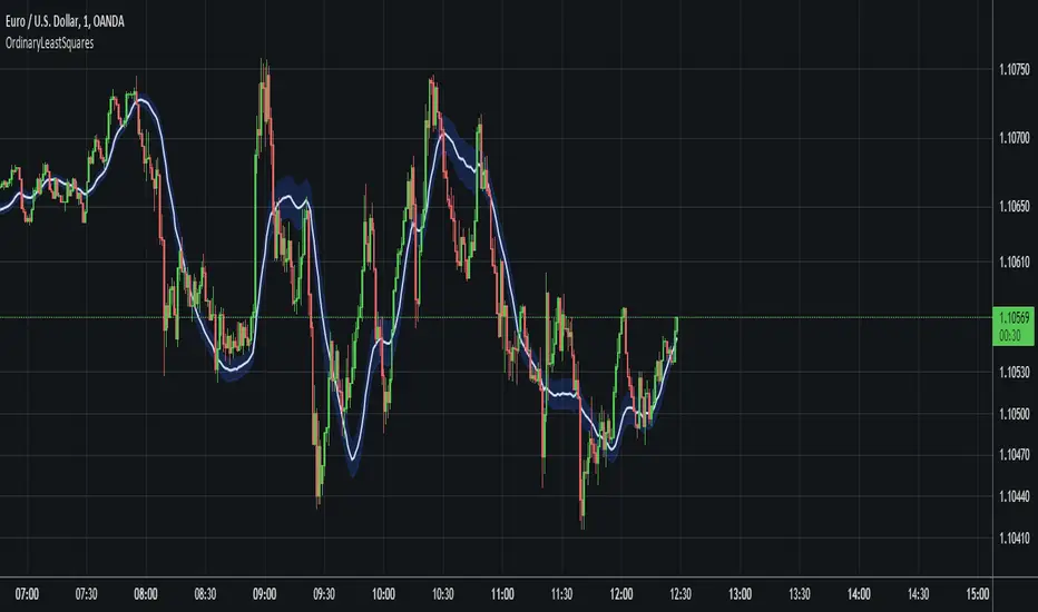
OrdinaryLeastSquaresLibrary "OrdinaryLeastSquares"
One of the most common ways to estimate the coefficients for a linear regression is to use the Ordinary Least Squares (OLS) method.
This library implements OLS in pine. This implementation can be used to fit a linear regression of multiple independent variables onto one dependent variable,
as long as the assumptions behind OLS hold.
solve_xtx_inv(x, y) Solve a linear system of equations using the Ordinary Least Squares method.
This function returns both the estimated OLS solution and a matrix that essentially measures the model stability (linear dependence between the columns of 'x').
NOTE: The latter is an intermediate step when estimating the OLS solution but is useful when calculating the covariance matrix and is returned here to save computation time
so that this step doesn't have to be calculated again when things like standard errors should be calculated.
Parameters:
x : The matrix containing the independent variables. Each column is regarded by the algorithm as one independent variable. The row count of 'x' and 'y' must match.
y : The matrix containing the dependent variable. This matrix can only contain one dependent variable and can therefore only contain one column. The row count of 'x' and 'y' must match.
Returns: Returns both the estimated OLS solution and a matrix that essentially measures the model stability (xtx_inv is equal to (X'X)^-1).
solve(x, y) Solve a linear system of equations using the Ordinary Least Squares method.
Parameters:
x : The matrix containing the independent variables. Each column is regarded by the algorithm as one independent variable. The row count of 'x' and 'y' must match.
y : The matrix containing the dependent variable. This matrix can only contain one dependent variable and can therefore only contain one column. The row count of 'x' and 'y' must match.
Returns: Returns the estimated OLS solution.
standard_errors(x, y, beta_hat, xtx_inv) Calculate the standard errors.
Parameters:
x : The matrix containing the independent variables. Each column is regarded by the algorithm as one independent variable. The row count of 'x' and 'y' must match.
y : The matrix containing the dependent variable. This matrix can only contain one dependent variable and can therefore only contain one column. The row count of 'x' and 'y' must match.
beta_hat : The Ordinary Least Squares (OLS) solution provided by solve_xtx_inv() or solve().
xtx_inv : This is (X'X)^-1, which means we take the transpose of the X matrix, multiply that the X matrix and then take the inverse of the result.
This essentially measures the linear dependence between the columns of the X matrix.
Returns: The standard errors.
estimate(x, beta_hat) Estimate the next step of a linear model.
Parameters:
x : The matrix containing the independent variables. Each column is regarded by the algorithm as one independent variable. The row count of 'x' and 'y' must match.
beta_hat : The Ordinary Least Squares (OLS) solution provided by solve_xtx_inv() or solve().
Returns: Returns the new estimate of Y based on the linear model.
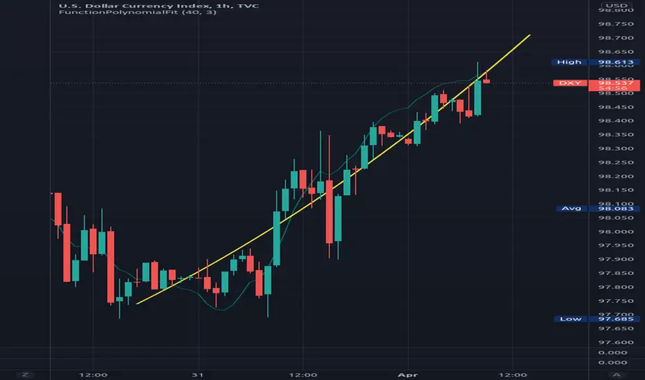
FunctionPolynomialFitLibrary "FunctionPolynomialFit"
Performs Polynomial Regression fit to data.
In statistics, polynomial regression is a form of regression analysis in which
the relationship between the independent variable x and the dependent variable
y is modelled as an nth degree polynomial in x.
reference:
en.wikipedia.org
www.bragitoff.com
gauss_elimination(A, m, n) Perform Gauss-Elimination and returns the Upper triangular matrix and solution of equations.
Parameters:
A : float matrix, data samples.
m : int, defval=na, number of rows.
n : int, defval=na, number of columns.
Returns: float array with coefficients.
polyfit(X, Y, degree) Fits a polynomial of a degree to (x, y) points.
Parameters:
X : float array, data sample x point.
Y : float array, data sample y point.
degree : int, defval=2, degree of the polynomial.
Returns: float array with coefficients.
note:
p(x) = p * x**deg + ... + p
interpolate(coeffs, x) interpolate the y position at the provided x.
Parameters:
coeffs : float array, coefficients of the polynomial.
x : float, position x to estimate y.
Returns: float.
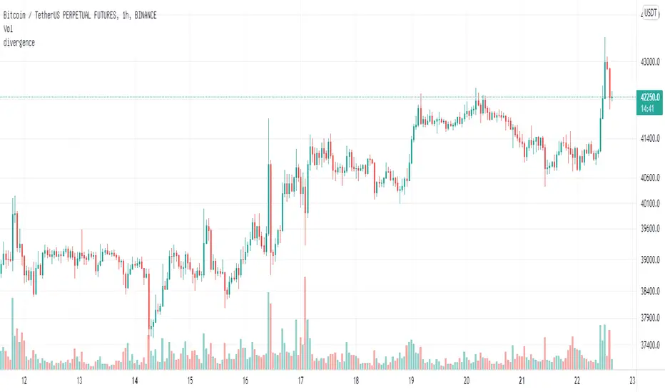
divergenceLibrary "divergence"
divergence: divergence algorithm with top and bottom kline tolerance
regular_bull(series, series, simple, simple, simple, simple, simple) regular_bull: regular bull divergence, lower low src but higher low osc
Parameters:
series : float src: the source series
series : float osc: the oscillator index
simple : int lbL: look back left
simple : int lbR: look back right
simple : int rangeL: min look back range
simple : int rangeU: max look back range
simple : int tolerance: the number of tolerant klines
Returns: array:
hidden_bull(series, series, simple, simple, simple, simple, simple) hidden_bull: hidden bull divergence, higher low src but lower low osc
Parameters:
series : float src: the source series
series : float osc: the oscillator index
simple : int lbL: look back left
simple : int lbR: look back right
simple : int rangeL: min look back range
simple : int rangeU: max look back range
simple : int tolerance: the number of tolerant klines
Returns: array:
regular_bear(series, series, simple, simple, simple, simple, simple) regular_bear: regular bear divergence, higher high src but lower high osc
Parameters:
series : float src: the source series
series : float osc: the oscillator index
simple : int lbL: look back left
simple : int lbR: look back right
simple : int rangeL: min look back range
simple : int rangeU: max look back range
simple : int tolerance: the number of tolerant klines
Returns: array:
hidden_bear(series, series, simple, simple, simple, simple, simple) hidden_bear: hidden bear divergence, lower high src but higher high osc
Parameters:
series : float src: the source series
series : float osc: the oscillator index
simple : int lbL: look back left
simple : int lbR: look back right
simple : int rangeL: min look back range
simple : int rangeU: max look back range
simple : int tolerance: the number of tolerant klines
Returns: array:
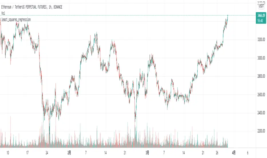
least_squares_regressionLibrary "least_squares_regression"
least_squares_regression: Least squares regression algorithm to find the optimal price interval for a given time period
basic_lsr(series, series, series) basic_lsr: Basic least squares regression algorithm
Parameters:
series : int t: time scale value array corresponding to price
series : float p: price scale value array corresponding to time
series : int array_size: the length of regression array
Returns: reg_slop, reg_intercept, reg_level, reg_stdev
trend_line_lsr(series, series, series, string, series, series) top_trend_line_lsr: Trend line fitting based on least square algorithm
Parameters:
series : int t: time scale value array corresponding to price
series : float p: price scale value array corresponding to time
series : int array_size: the length of regression array
string : reg_type: regression type in 'top' and 'bottom'
series : int max_iter: maximum fitting iterations
series : int min_points: the threshold of regression point numbers
Returns: reg_slop, reg_intercept, reg_level, reg_stdev, reg_point_num
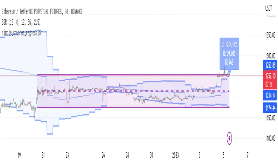
simple_squares_regressionLibrary "simple_squares_regression"
simple_squares_regression: simple squares regression algorithm to find the optimal price interval for a given time period
basic_ssr(series, series, series) basic_ssr: Basic simple squares regression algorithm
Parameters:
series : float src: the regression source such as close
series : int region_forward: number of candle lines at the right end of the regression region from the current candle line
series : int region_len: the length of regression region
Returns: left_loc, right_loc, reg_val, reg_std, reg_max_offset
search_ssr(series, series, series, series) search_ssr: simple squares regression region search algorithm
Parameters:
series : float src: the regression source such as close
series : int max_forward: max number of candle lines at the right end of the regression region from the current candle line
series : int region_lower: the lower length of regression region
series : int region_upper: the upper length of regression region
Returns: left_loc, right_loc, reg_val, reg_level, reg_std_err, reg_max_offset
on_balance_volumeLibrary "on_balance_volume"
on_balance_volume: custom on balance volume
obv_diff(string, simple) obv_diff: custom on balance volume diff version
Parameters:
string : type: the moving average type of on balance volume
simple : int len: the moving average length of on balance volume
Returns: obv_diff: custom on balance volume diff value
obv_diff_norm(string, simple) obv_diff_norm: custom normalized on balance volume diff version
Parameters:
string : type: the moving average type of on balance volume
simple : int len: the moving average length of on balance volume
Returns: obv_diff: custom normalized on balance volume diff value

moving_averageLibrary "moving_average"
moving_average: moving average variants
variant(string, series, simple) variant: moving average variants
Parameters:
string : type: type in
series : float src: the source series of moving average
simple : int len: the length of moving average
Returns: float: the moving average variant value

ConditionalAverages█ OVERVIEW
This library is a Pine Script™ programmer’s tool containing functions that average values selectively.
█ CONCEPTS
Averaging can be useful to smooth out unstable readings in the data set, provide a benchmark to see the underlying trend of the data, or to provide a general expectancy of values in establishing a central tendency. Conventional averaging techniques tend to apply indiscriminately to all values in a fixed window, but it can sometimes be useful to average values only when a specific condition is met. As conditional averaging works on specific elements of a dataset, it can help us derive more context-specific conclusions. This library offers a collection of averaging methods that not only accomplish these tasks, but also exploit the efficiencies of the Pine Script™ runtime by foregoing unnecessary and resource-intensive for loops.
█ NOTES
To Loop or Not to Loop
Though for and while loops are essential programming tools, they are often unnecessary in Pine Script™. This is because the Pine Script™ runtime already runs your scripts in a loop where it executes your code on each bar of the dataset. Pine Script™ programmers who understand how their code executes on charts can use this to their advantage by designing loop-less code that will run orders of magnitude faster than functionally identical code using loops. Most of this library's function illustrate how you can achieve loop-less code to process past values. See the User Manual page on loops for more information. If you are looking for ways to measure execution time for you scripts, have a look at our LibraryStopwatch library .
Our `avgForTimeWhen()` and `totalForTimeWhen()` are exceptions in the library, as they use a while structure. Only a few iterations of the loop are executed on each bar, however, as its only job is to remove the few elements in the array that are outside the moving window defined by a time boundary.
Cumulating and Summing Conditionally
The ta.cum() or math.sum() built-in functions can be used with ternaries that select only certain values. In our `avgWhen(src, cond)` function, for example, we use this technique to cumulate only the occurrences of `src` when `cond` is true:
float cumTotal = ta.cum(cond ? src : 0) We then use:
float cumCount = ta.cum(cond ? 1 : 0) to calculate the number of occurrences where `cond` is true, which corresponds to the quantity of values cumulated in `cumTotal`.
Building Custom Series With Arrays
The advent of arrays in Pine has enabled us to build our custom data series. Many of this library's functions use arrays for this purpose, saving newer values that come in when a condition is met, and discarding the older ones, implementing a queue .
`avgForTimeWhen()` and `totalForTimeWhen()`
These two functions warrant a few explanations. They operate on a number of values included in a moving window defined by a timeframe expressed in milliseconds. We use a 1D timeframe in our example code. The number of bars included in the moving window is unknown to the programmer, who only specifies the period of time defining the moving window. You can thus use `avgForTimeWhen()` to calculate a rolling moving average for the last 24 hours, for example, that will work whether the chart is using a 1min or 1H timeframe. A 24-hour moving window will typically contain many more values on a 1min chart that on a 1H chart, but their calculated average will be very close.
Problems will arise on non-24x7 markets when large time gaps occur between chart bars, as will be the case across holidays or trading sessions. For example, if you were using a 24H timeframe and there is a two-day gap between two bars, then no chart bars would fit in the moving window after the gap. The `minBars` parameter mitigates this by guaranteeing that a minimum number of bars are always included in the calculation, even if including those bars requires reaching outside the prescribed timeframe. We use a minimum value of 10 bars in the example code.
Using var in Constant Declarations
In the past, we have been using var when initializing so-called constants in our scripts, which as per the Style Guide 's recommendations, we identify using UPPER_SNAKE_CASE. It turns out that var variables incur slightly superior maintenance overhead in the Pine Script™ runtime, when compared to variables initialized on each bar. We thus no longer use var to declare our "int/float/bool" constants, but still use it when an initialization on each bar would require too much time, such as when initializing a string or with a heavy function call.
Look first. Then leap.
█ FUNCTIONS
avgWhen(src, cond)
Gathers values of the source when a condition is true and averages them over the total number of occurrences of the condition.
Parameters:
src : (series int/float) The source of the values to be averaged.
cond : (series bool) The condition determining when a value will be included in the set of values to be averaged.
Returns: (float) A cumulative average of values when a condition is met.
avgWhenLast(src, cond, cnt)
Gathers values of the source when a condition is true and averages them over a defined number of occurrences of the condition.
Parameters:
src : (series int/float) The source of the values to be averaged.
cond : (series bool) The condition determining when a value will be included in the set of values to be averaged.
cnt : (simple int) The quantity of last occurrences of the condition for which to average values.
Returns: (float) The average of `src` for the last `x` occurrences where `cond` is true.
avgWhenInLast(src, cond, cnt)
Gathers values of the source when a condition is true and averages them over the total number of occurrences during a defined number of bars back.
Parameters:
src : (series int/float) The source of the values to be averaged.
cond : (series bool) The condition determining when a value will be included in the set of values to be averaged.
cnt : (simple int) The quantity of bars back to evaluate.
Returns: (float) The average of `src` in last `cnt` bars, but only when `cond` is true.
avgSince(src, cond)
Averages values of the source since a condition was true.
Parameters:
src : (series int/float) The source of the values to be averaged.
cond : (series bool) The condition determining when the average is reset.
Returns: (float) The average of `src` since `cond` was true.
avgForTimeWhen(src, ms, cond, minBars)
Averages values of `src` when `cond` is true, over a moving window of length `ms` milliseconds.
Parameters:
src : (series int/float) The source of the values to be averaged.
ms : (simple int) The time duration in milliseconds defining the size of the moving window.
cond : (series bool) The condition determining which values are included. Optional.
minBars : (simple int) The minimum number of values to keep in the moving window. Optional.
Returns: (float) The average of `src` when `cond` is true in the moving window.
totalForTimeWhen(src, ms, cond, minBars)
Sums values of `src` when `cond` is true, over a moving window of length `ms` milliseconds.
Parameters:
src : (series int/float) The source of the values to be summed.
ms : (simple int) The time duration in milliseconds defining the size of the moving window.
cond : (series bool) The condition determining which values are included. Optional.
minBars : (simple int) The minimum number of values to keep in the moving window. Optional.
Returns: (float) The sum of `src` when `cond` is true in the moving window.

MathProbabilityDistributionLibrary "MathProbabilityDistribution"
Probability Distribution Functions.
name(idx) Indexed names helper function.
Parameters:
idx : int, position in the range (0, 6).
Returns: string, distribution name.
usage:
.name(1)
Notes:
(0) => 'StdNormal'
(1) => 'Normal'
(2) => 'Skew Normal'
(3) => 'Student T'
(4) => 'Skew Student T'
(5) => 'GED'
(6) => 'Skew GED'
zscore(position, mean, deviation) Z-score helper function for x calculation.
Parameters:
position : float, position.
mean : float, mean.
deviation : float, standard deviation.
Returns: float, z-score.
usage:
.zscore(1.5, 2.0, 1.0)
std_normal(position) Standard Normal Distribution.
Parameters:
position : float, position.
Returns: float, probability density.
usage:
.std_normal(0.6)
normal(position, mean, scale) Normal Distribution.
Parameters:
position : float, position in the distribution.
mean : float, mean of the distribution, default=0.0 for standard distribution.
scale : float, scale of the distribution, default=1.0 for standard distribution.
Returns: float, probability density.
usage:
.normal(0.6)
skew_normal(position, skew, mean, scale) Skew Normal Distribution.
Parameters:
position : float, position in the distribution.
skew : float, skewness of the distribution.
mean : float, mean of the distribution, default=0.0 for standard distribution.
scale : float, scale of the distribution, default=1.0 for standard distribution.
Returns: float, probability density.
usage:
.skew_normal(0.8, -2.0)
ged(position, shape, mean, scale) Generalized Error Distribution.
Parameters:
position : float, position.
shape : float, shape.
mean : float, mean, default=0.0 for standard distribution.
scale : float, scale, default=1.0 for standard distribution.
Returns: float, probability.
usage:
.ged(0.8, -2.0)
skew_ged(position, shape, skew, mean, scale) Skew Generalized Error Distribution.
Parameters:
position : float, position.
shape : float, shape.
skew : float, skew.
mean : float, mean, default=0.0 for standard distribution.
scale : float, scale, default=1.0 for standard distribution.
Returns: float, probability.
usage:
.skew_ged(0.8, 2.0, 1.0)
student_t(position, shape, mean, scale) Student-T Distribution.
Parameters:
position : float, position.
shape : float, shape.
mean : float, mean, default=0.0 for standard distribution.
scale : float, scale, default=1.0 for standard distribution.
Returns: float, probability.
usage:
.student_t(0.8, 2.0, 1.0)
skew_student_t(position, shape, skew, mean, scale) Skew Student-T Distribution.
Parameters:
position : float, position.
shape : float, shape.
skew : float, skew.
mean : float, mean, default=0.0 for standard distribution.
scale : float, scale, default=1.0 for standard distribution.
Returns: float, probability.
usage:
.skew_student_t(0.8, 2.0, 1.0)
select(distribution, position, mean, scale, shape, skew, log) Conditional Distribution.
Parameters:
distribution : string, distribution name.
position : float, position.
mean : float, mean, default=0.0 for standard distribution.
scale : float, scale, default=1.0 for standard distribution.
shape : float, shape.
skew : float, skew.
log : bool, if true apply log() to the result.
Returns: float, probability.
usage:
.select('StdNormal', __CYCLE4F__, log=true)