FunctionSurvivalEstimationLibrary "FunctionSurvivalEstimation"
The Survival Estimation function, also known as Kaplan-Meier estimation or product-limit method, is a statistical technique used to estimate the survival probability of an individual over time. It's commonly used in medical research and epidemiology to analyze the survival rates of patients with different treatments, diseases, or risk factors.
What does it do?
The Survival Estimation function takes into account censored observations (i.e., individuals who are still alive at a certain point) and calculates the probability that an individual will survive beyond a specific time period. It's particularly useful when dealing with right-censoring, where some subjects are lost to follow-up or have not experienced the event of interest by the end of the study.
Interpretation
The Survival Estimation function provides a plot of the estimated survival probability over time, which can be used to:
1. Compare survival rates between different groups (e.g., treatment arms)
2. Identify patterns in the data that may indicate differences in mortality or disease progression
3. Make predictions about future outcomes based on historical data
4. In a trading context it may be used to ascertain the survival ratios of trading under specific conditions.
Reference:
www.global-developments.org
"Beyond GDP" ~ www.aeaweb.org
en.wikipedia.org
www.kdnuggets.com
survival_probability(alive_at_age, initial_alive)
Kaplan-Meier Survival Estimator.
Parameters:
alive_at_age (int) : The number of subjects still alive at a age.
initial_alive (int) : The Total number of initial subjects.
Returns: The probability that a subject lives longer than a certain age.
utility(c, l)
Captures the utility value from consumption and leisure.
Parameters:
c (float) : Consumption.
l (float) : Leisure.
Returns: Utility value from consumption and leisure.
welfare_utility(age, b, u, s)
Calculate the welfare utility value based age, basic needs and social interaction.
Parameters:
age (int) : Age of the subject.
b (float) : Value representing basic needs (food, shelter..).
u (float) : Value representing overall well-being and happiness.
s (float) : Value representing social interaction and connection with others.
Returns: Welfare utility value.
expected_lifetime_welfare(beta, consumption, leisure, alive_data, expectation)
Calculates the expected lifetime welfare of an individual based on their consumption, leisure, and survival probability over time.
Parameters:
beta (float) : Discount factor.
consumption (array) : List of consumption values at each step of the subjects life.
leisure (array) : List of leisure values at each step of the subjects life.
alive_data (array) : List of subjects alive at each age, the first element is the total or initial number of subjects.
expectation (float) : Optional, `defaut=1.0`. Expectation or weight given to this calculation.
Returns: Expected lifetime welfare value.
MATH

PineVersatilitiesBundleLibrary "PineVersatilitiesBundle"
Versatilities (aka, Versatile Utilities) Pack includes:
- Eighteen Price Variants bundled in a Map,
- Nine Smoothing Variants bundled in a Map,
- Visualisations that indicate on both - pane and chart.
price_variants(lb)
Computes Several different averages using current and previous OHLC values
Parameters:
lb (int) : - lookback distance for combining OHLC values from the past with the present
Returns: Map of Eighteen Uncommon Combinations of single and two-bar OHLC averages (rounded-to-mintick)
dynamic_MA(masrc, malen, lsmaoff, almasgm, almaoff, almaflr)
Dynamically computes Eight different MAs and returns a Map containing Nine MAs
Parameters:
masrc (float) : source series to compute MA
malen (simple int) : lookback distance for MA
lsmaoff (simple int) : optional LSMA offset - default is 0
almasgm (simple float) : optional ALMA sigma - default is 5
almaoff (simple float) : optional ALMA offset - default is 0.5
almaflr (simple bool) : optional ALMA floor flag - default is false
Returns: Map of MAs - 'ALMA', 'EMA', 'HMA', 'LSMA', 'RMA', 'SMA', 'SWMA', 'WMA', 'ALL' (rounded-to-mintick)

NR_VersatilitiesLibrary "NR_Versatilities"
Versatilities (aka, Versatile Utilities) includes:
- Seventeen Price Variants returned as a tuple,
- Eight Smoothing functions rolled into one,
- Pick any Past Value from any series with offset,
- Or just the previous value from any series.
pastVal(src, len)
Fetches past value from src that came len distance ago
Parameters:
src (float) : source series
len (int) : lookback distance - (optional) default is 1
Returns: latest src if len <= 0, else src
previous(src)
Fetches past value from src that came len distance ago
Parameters:
src (float) : source series
Returns: previous value in the series if found, else current value
price_variants()
Computes Several different averages using current and previous OHLC values
Returns: Seventeen Uncommon Average Price Combinations
dynamic_MA(matyp, masrc, malen, lsmaoff, almasgm, almaoff, almaflr)
Dynamically computes Eight different MAs on-demand individually, or an average of all taken together
Parameters:
matyp (string) : pick one of these MAs - ALMA, EMA, HMA, LSMA, RMA, SMA, SWMA, WMA, ALL
masrc (float) : source series to compute MA
malen (simple int) : lookback distance for MA
lsmaoff (simple int) : optional LSMA offset - default is 0
almasgm (simple float) : optional ALMA sigma - default is 5
almaoff (simple float) : optional ALMA offset - default is 0.5
almaflr (simple bool) : optional ALMA floor flag - default is false
Returns: MA series for chosen type or, an average of all of them, if chosen so

TimeframeUtilsCustomLibrary "TimeframeUtilsCustom"
Timeframe utilities library
f_timeframe_to_minutes(tf)
Converts timeframe string to minutes
Parameters:
tf (string) : String representation of timeframe
Returns: Number of minutes in the given timeframe
f_bars_for_hours(timeframe_minutes, hours)
Calculate number of bars for a specified time period
Parameters:
timeframe_minutes (int) : Current timeframe in minutes
hours (int) : Number of hours to calculate bars for
Returns: Number of bars representing the specified hours
f_bars_for_days(timeframe_minutes, days)
Calculate number of bars for a specified number of days
Parameters:
timeframe_minutes (int) : Current timeframe in minutes
days (int) : Number of days to calculate bars for
Returns: Number of bars representing the specified days

rate_of_changeLibrary "rate_of_change"
// @description: Applies ROC algorithm to any pair of values.
// This library function is used to scale change of value (price, volume) to a percentage value, just as the ROC indicator would do. It is good practice to scale arbitrary ranges to set boundaries when you try to train statistical model.
rateOfChange(value, base, hardlimit)
This function is a helper to scale a value change to its percentage value.
Parameters:
value (float)
base (float)
hardlimit (int)
Returns: per: A float comprised between 0 and 100

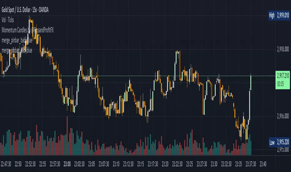
merge_pinbar_babyblueLibrary "merge_pinbar_babyblue"
merge_pinbar: merge bars and check whether the bar is a pinbar
merge_pinbar_babyblue(period, max_bars)
merge_pinbar: merge bars and check whether the bar is a pinbar
Parameters:
period (simple int)
max_bars (simple int)
Returns: array:
DynamicMALibrary "DynamicMA"
Dynamic Moving Averages Library
Introduction
The Dynamic Moving Averages Library is a specialized collection of custom built functions designed to calculate moving averages dynamically, beginning from the first available bar. Unlike standard moving averages, which rely on fixed length lookbacks, this library ensures that indicators remain fully functional from the very first data point, making it an essential tool for analysing assets with short time series or limited historical data.
This approach allows traders and developers to build robust indicators that do not require a preset amount of historical data before generating meaningful outputs. It is particularly advantageous for:
Newly listed assets with minimal price history.
High-timeframe trading, where large lookback periods can lead to delayed or missing data.
By eliminating the constraints of fixed lookback periods, this library enables the seamless construction of trend indicators, smoothing functions, and hybrid models that adapt instantly to market conditions.
Comprehensive Set of Custom Moving Averages
The library includes a wide range of custom dynamic moving averages, each designed for specific analytical use cases:
SMA (Simple Moving Average) – The fundamental moving average, dynamically computed.
EMA (Exponential Moving Average) – Adaptive smoothing for better trend tracking.
DEMA (Double Exponential Moving Average) – Faster trend detection with reduced lag.
TEMA (Triple Exponential Moving Average) – Even more responsive than DEMA.
WMA (Weighted Moving Average) – Emphasizes recent price action while reducing noise.
VWMA (Volume Weighted Moving Average) – Accounts for volume to give more weight to high-volume periods.
HMA (Hull Moving Average) – A superior smoothing method with low lag.
SMMA (Smoothed Moving Average) – A hybrid approach between SMA and EMA.
LSMA (Least Squares Moving Average) – Uses linear regression for trend detection.
RMA (Relative Moving Average) – Used in RSI-based calculations for smooth momentum readings.
ALMA (Arnaud Legoux Moving Average) – A Gaussian-weighted MA for superior signal clarity.
Hyperbolic MA (HyperMA) – A mathematically optimized averaging method with dynamic weighting.
Each function dynamically adjusts its calculation length to match the available bar count, ensuring instant functionality on all assets.
Fully Optimized for Pine Script v6
This library is built on Pine Script v6, ensuring compatibility with modern TradingView indicators and scripts. It includes exportable functions for seamless integration into custom indicators, making it easy to develop trend-following models, volatility filters, and adaptive risk-management systems.
Why Use Dynamic Moving Averages?
Traditional moving averages suffer from a common limitation: they require a fixed historical window to generate meaningful values. This poses several problems:
New Assets Have No Historical Data - If an asset has only been trading for a short period, traditional moving averages may not be able to generate valid signals.
High Timeframes Require Massive Lookbacks - On 1W or 1M charts, a 200-period SMA would require 200 weeks or months of data, making it unusable on newer assets.
Delayed Signal Initialization - Standard indicators often take dozens of bars to stabilize, reducing effectiveness when trading new trends.
The Dynamic Moving Averages Library eliminates these issues by ensuring that every function:
Starts calculation from bar one, using available data instead of waiting for a lookback period.
Adapts dynamically across timeframes, making it equally effective on low or high timeframes.
Allows smoother, more responsive trend tracking, particularly useful for volatile or low-liquidity assets.
This flexibility makes it indispensable for custom script developers, quantitative analysts, and discretionary traders looking to build more adaptive and resilient indicators.
Final Summary
The Dynamic Moving Averages Library is a versatile and powerful set of functions designed to overcome the limitations of fixed-lookback indicators. By dynamically adjusting the calculation length from the first bar, this library ensures that moving averages remain fully functional across all timeframes and asset types, making it an essential tool for traders and developers alike.
With built-in adaptability, low-lag smoothing, and support for multiple moving average types, this library unlocks new possibilities for quantitative trading and strategy development - especially for assets with short price histories or those traded on higher timeframes.
For traders looking to enhance signal reliability, minimize lag, and build adaptable trading systems, the Dynamic Moving Averages Library provides an efficient and flexible solution.
SMA(sourceData, maxLength)
Dynamic SMA
Parameters:
sourceData (float)
maxLength (int)
EMA(src, length)
Dynamic EMA
Parameters:
src (float)
length (int)
DEMA(src, length)
Dynamic DEMA
Parameters:
src (float)
length (int)
TEMA(src, length)
Dynamic TEMA
Parameters:
src (float)
length (int)
WMA(src, length)
Dynamic WMA
Parameters:
src (float)
length (int)
HMA(src, length)
Dynamic HMA
Parameters:
src (float)
length (int)
VWMA(src, volsrc, length)
Dynamic VWMA
Parameters:
src (float)
volsrc (float)
length (int)
SMMA(src, length)
Dynamic SMMA
Parameters:
src (float)
length (int)
LSMA(src, length, offset)
Dynamic LSMA
Parameters:
src (float)
length (int)
offset (int)
RMA(src, length)
Dynamic RMA
Parameters:
src (float)
length (int)
ALMA(src, length, offset_sigma, sigma)
Dynamic ALMA
Parameters:
src (float)
length (int)
offset_sigma (float)
sigma (float)
HyperMA(src, length)
Dynamic HyperbolicMA
Parameters:
src (float)
length (int)

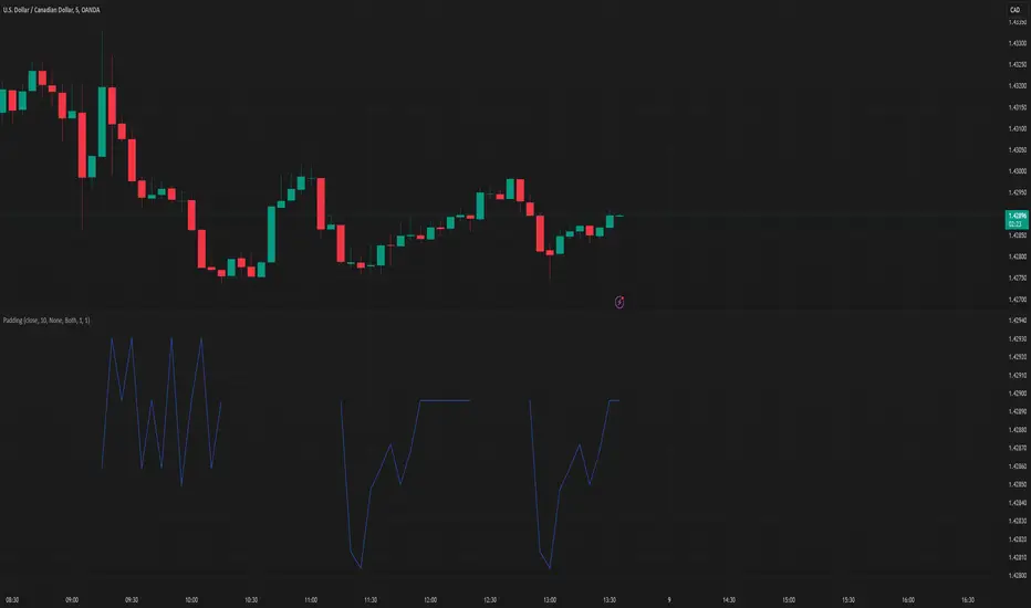
PaddingThe Padding library is a comprehensive and flexible toolkit designed to extend time series data within TradingView, making it an indispensable resource for advanced signal processing tasks such as FFT, filtering, convolution, and wavelet analysis. At its core, the library addresses the common challenge of edge effects by "padding" your data—that is, by appending additional data points beyond the natural boundaries of your original dataset. This extension not only mitigates the distortions that can occur at the endpoints but also helps to maintain the integrity of various transformations and calculations performed on the series. The library accomplishes this while preserving the ordering of your data, ensuring that the most recent point always resides at index 0.
Central to the functionality of this library are two key enumerations: Direction and PaddingType. The Direction enum determines where the padding will be applied. You can choose to extend the data in the forward direction (ahead of the current values), in the backward direction (behind the current values), or in both directions simultaneously. The PaddingType enum defines the specific method used for extending the data. The library supports several methods—including symmetric, reflect, periodic, antisymmetric, antireflect, smooth, constant, and zero padding—each of which has been implemented to suit different analytical scenarios. For instance, symmetric padding mirrors the original data across its boundaries, while reflect padding continues the trend by reflecting around endpoint values. Periodic padding repeats the data, and antisymmetric padding mirrors the data with alternating signs to counterbalance it. The antireflect and smooth methods take into account the derivatives of your data, thereby extending the series in a way that preserves or smoothly continues these derivative values. Constant and zero padding simply extend the series using fixed endpoint values or zeros. Together, these enums allow you to fine-tune how your data is extended, ensuring that the padding method aligns with the specific requirements of your analysis.
The library is designed to work with both single variable inputs and array inputs. When using array-based methods—particularly with the antireflect and smooth padding types—please note that the implementation intentionally discards the last data point as a result of the delta computation process. This behavior is an important consideration when integrating the library into your TradingView studies, as it affects the overall data length of the padded series. Despite this, the library’s structure and documentation make it straightforward to incorporate into your existing scripts. You simply provide your data source, define the length of your data window, and select the desired padding type and direction, along with any optional parameters to control the extent of the padding (using both_period, forward_period, or backward_period).
In practical application, the Padding library enables you to extend historical data beyond its original range in a controlled and predictable manner. This is particularly useful when preparing datasets for further signal processing, as it helps to reduce artifacts that can otherwise compromise the results of your analytical routines. Whether you are an experienced Pine Script developer or a trader exploring advanced data analysis techniques, this library offers a robust solution that enhances the reliability and accuracy of your studies by ensuring your algorithms operate on a more complete and well-prepared dataset.
Library "Padding"
A comprehensive library for padding time series data with various methods. Supports both single variable and array inputs, with flexible padding directions and periods. Designed for signal processing applications including FFT, filtering, convolution, and wavelets. All methods maintain data ordering with most recent point at index 0.
symmetric(source, series_length, direction, both_period, forward_period, backward_period)
Applies symmetric padding by mirroring the input data across boundaries
Parameters:
source (float) : Input value to pad from
series_length (int) : Length of the data window
direction (series Direction) : Direction to apply padding
both_period (int) : Optional - periods to pad in both directions. Overrides forward_period and backward_period if specified
forward_period (int) : Optional - periods to pad forward. Defaults to series_length if not specified
backward_period (int) : Optional - periods to pad backward. Defaults to series_length if not specified
Returns: Array ordered with most recent point at index 0, containing original data with symmetric padding applied
method symmetric(source, direction, both_period, forward_period, backward_period)
Applies symmetric padding to an array by mirroring the data across boundaries
Namespace types: array
Parameters:
source (array) : Array of values to pad
direction (series Direction) : Direction to apply padding
both_period (int) : Optional - periods to pad in both directions. Overrides forward_period and backward_period if specified
forward_period (int) : Optional - periods to pad forward. Defaults to array length if not specified
backward_period (int) : Optional - periods to pad backward. Defaults to array length if not specified
Returns: Array ordered with most recent point at index 0, containing original data with symmetric padding applied
reflect(source, series_length, direction, both_period, forward_period, backward_period)
Applies reflect padding by continuing trends through reflection around endpoint values
Parameters:
source (float) : Input value to pad from
series_length (int) : Length of the data window
direction (series Direction) : Direction to apply padding
both_period (int) : Optional - periods to pad in both directions. Overrides forward_period and backward_period if specified
forward_period (int) : Optional - periods to pad forward. Defaults to series_length if not specified
backward_period (int) : Optional - periods to pad backward. Defaults to series_length if not specified
Returns: Array ordered with most recent point at index 0, containing original data with reflect padding applied
method reflect(source, direction, both_period, forward_period, backward_period)
Applies reflect padding to an array by continuing trends through reflection around endpoint values
Namespace types: array
Parameters:
source (array) : Array of values to pad
direction (series Direction) : Direction to apply padding
both_period (int) : Optional - periods to pad in both directions. Overrides forward_period and backward_period if specified
forward_period (int) : Optional - periods to pad forward. Defaults to array length if not specified
backward_period (int) : Optional - periods to pad backward. Defaults to array length if not specified
Returns: Array ordered with most recent point at index 0, containing original data with reflect padding applied
periodic(source, series_length, direction, both_period, forward_period, backward_period)
Applies periodic padding by repeating the input data
Parameters:
source (float) : Input value to pad from
series_length (int) : Length of the data window
direction (series Direction) : Direction to apply padding
both_period (int) : Optional - periods to pad in both directions. Overrides forward_period and backward_period if specified
forward_period (int) : Optional - periods to pad forward. Defaults to series_length if not specified
backward_period (int) : Optional - periods to pad backward. Defaults to series_length if not specified
Returns: Array ordered with most recent point at index 0, containing original data with periodic padding applied
method periodic(source, direction, both_period, forward_period, backward_period)
Applies periodic padding to an array by repeating the data
Namespace types: array
Parameters:
source (array) : Array of values to pad
direction (series Direction) : Direction to apply padding
both_period (int) : Optional - periods to pad in both directions. Overrides forward_period and backward_period if specified
forward_period (int) : Optional - periods to pad forward. Defaults to array length if not specified
backward_period (int) : Optional - periods to pad backward. Defaults to array length if not specified
Returns: Array ordered with most recent point at index 0, containing original data with periodic padding applied
antisymmetric(source, series_length, direction, both_period, forward_period, backward_period)
Applies antisymmetric padding by mirroring data and alternating signs
Parameters:
source (float) : Input value to pad from
series_length (int) : Length of the data window
direction (series Direction) : Direction to apply padding
both_period (int) : Optional - periods to pad in both directions. Overrides forward_period and backward_period if specified
forward_period (int) : Optional - periods to pad forward. Defaults to series_length if not specified
backward_period (int) : Optional - periods to pad backward. Defaults to series_length if not specified
Returns: Array ordered with most recent point at index 0, containing original data with antisymmetric padding applied
method antisymmetric(source, direction, both_period, forward_period, backward_period)
Applies antisymmetric padding to an array by mirroring data and alternating signs
Namespace types: array
Parameters:
source (array) : Array of values to pad
direction (series Direction) : Direction to apply padding
both_period (int) : Optional - periods to pad in both directions. Overrides forward_period and backward_period if specified
forward_period (int) : Optional - periods to pad forward. Defaults to array length if not specified
backward_period (int) : Optional - periods to pad backward. Defaults to array length if not specified
Returns: Array ordered with most recent point at index 0, containing original data with antisymmetric padding applied
antireflect(source, series_length, direction, both_period, forward_period, backward_period)
Applies antireflect padding by reflecting around endpoints while preserving derivatives
Parameters:
source (float) : Input value to pad from
series_length (int) : Length of the data window
direction (series Direction) : Direction to apply padding
both_period (int) : Optional - periods to pad in both directions. Overrides forward_period and backward_period if specified
forward_period (int) : Optional - periods to pad forward. Defaults to series_length if not specified
backward_period (int) : Optional - periods to pad backward. Defaults to series_length if not specified
Returns: Array ordered with most recent point at index 0, containing original data with antireflect padding applied
method antireflect(source, direction, both_period, forward_period, backward_period)
Applies antireflect padding to an array by reflecting around endpoints while preserving derivatives
Namespace types: array
Parameters:
source (array) : Array of values to pad
direction (series Direction) : Direction to apply padding
both_period (int) : Optional - periods to pad in both directions. Overrides forward_period and backward_period if specified
forward_period (int) : Optional - periods to pad forward. Defaults to array length if not specified
backward_period (int) : Optional - periods to pad backward. Defaults to array length if not specified
Returns: Array ordered with most recent point at index 0, containing original data with antireflect padding applied. Note: Last data point is lost when using array input
smooth(source, series_length, direction, both_period, forward_period, backward_period)
Applies smooth padding by extending with constant derivatives from endpoints
Parameters:
source (float) : Input value to pad from
series_length (int) : Length of the data window
direction (series Direction) : Direction to apply padding
both_period (int) : Optional - periods to pad in both directions. Overrides forward_period and backward_period if specified
forward_period (int) : Optional - periods to pad forward. Defaults to series_length if not specified
backward_period (int) : Optional - periods to pad backward. Defaults to series_length if not specified
Returns: Array ordered with most recent point at index 0, containing original data with smooth padding applied
method smooth(source, direction, both_period, forward_period, backward_period)
Applies smooth padding to an array by extending with constant derivatives from endpoints
Namespace types: array
Parameters:
source (array) : Array of values to pad
direction (series Direction) : Direction to apply padding
both_period (int) : Optional - periods to pad in both directions. Overrides forward_period and backward_period if specified
forward_period (int) : Optional - periods to pad forward. Defaults to array length if not specified
backward_period (int) : Optional - periods to pad backward. Defaults to array length if not specified
Returns: Array ordered with most recent point at index 0, containing original data with smooth padding applied. Note: Last data point is lost when using array input
constant(source, series_length, direction, both_period, forward_period, backward_period)
Applies constant padding by extending endpoint values
Parameters:
source (float) : Input value to pad from
series_length (int) : Length of the data window
direction (series Direction) : Direction to apply padding
both_period (int) : Optional - periods to pad in both directions. Overrides forward_period and backward_period if specified
forward_period (int) : Optional - periods to pad forward. Defaults to series_length if not specified
backward_period (int) : Optional - periods to pad backward. Defaults to series_length if not specified
Returns: Array ordered with most recent point at index 0, containing original data with constant padding applied
method constant(source, direction, both_period, forward_period, backward_period)
Applies constant padding to an array by extending endpoint values
Namespace types: array
Parameters:
source (array) : Array of values to pad
direction (series Direction) : Direction to apply padding
both_period (int) : Optional - periods to pad in both directions. Overrides forward_period and backward_period if specified
forward_period (int) : Optional - periods to pad forward. Defaults to array length if not specified
backward_period (int) : Optional - periods to pad backward. Defaults to array length if not specified
Returns: Array ordered with most recent point at index 0, containing original data with constant padding applied
zero(source, series_length, direction, both_period, forward_period, backward_period)
Applies zero padding by extending with zeros
Parameters:
source (float) : Input value to pad from
series_length (int) : Length of the data window
direction (series Direction) : Direction to apply padding
both_period (int) : Optional - periods to pad in both directions. Overrides forward_period and backward_period if specified
forward_period (int) : Optional - periods to pad forward. Defaults to series_length if not specified
backward_period (int) : Optional - periods to pad backward. Defaults to series_length if not specified
Returns: Array ordered with most recent point at index 0, containing original data with zero padding applied
method zero(source, direction, both_period, forward_period, backward_period)
Applies zero padding to an array by extending with zeros
Namespace types: array
Parameters:
source (array) : Array of values to pad
direction (series Direction) : Direction to apply padding
both_period (int) : Optional - periods to pad in both directions. Overrides forward_period and backward_period if specified
forward_period (int) : Optional - periods to pad forward. Defaults to array length if not specified
backward_period (int) : Optional - periods to pad backward. Defaults to array length if not specified
Returns: Array ordered with most recent point at index 0, containing original data with zero padding applied
pad_data(source, series_length, padding_type, direction, both_period, forward_period, backward_period)
Generic padding function that applies specified padding type to input data
Parameters:
source (float) : Input value to pad from
series_length (int) : Length of the data window
padding_type (series PaddingType) : Type of padding to apply (see PaddingType enum)
direction (series Direction) : Direction to apply padding
both_period (int) : Optional - periods to pad in both directions. Overrides forward_period and backward_period if specified
forward_period (int) : Optional - periods to pad forward. Defaults to series_length if not specified
backward_period (int) : Optional - periods to pad backward. Defaults to series_length if not specified
Returns: Array ordered with most recent point at index 0, containing original data with specified padding applied
method pad_data(source, padding_type, direction, both_period, forward_period, backward_period)
Generic padding function that applies specified padding type to array input
Namespace types: array
Parameters:
source (array) : Array of values to pad
padding_type (series PaddingType) : Type of padding to apply (see PaddingType enum)
direction (series Direction) : Direction to apply padding
both_period (int) : Optional - periods to pad in both directions. Overrides forward_period and backward_period if specified
forward_period (int) : Optional - periods to pad forward. Defaults to array length if not specified
backward_period (int) : Optional - periods to pad backward. Defaults to array length if not specified
Returns: Array ordered with most recent point at index 0, containing original data with specified padding applied. Note: Last data point is lost when using antireflect or smooth padding types
make_padded_data(source, series_length, padding_type, direction, both_period, forward_period, backward_period)
Creates a window-based padded data series that updates with each new value. WARNING: Function must be called on every bar for consistency. Do not use in scopes where it may not execute on every bar.
Parameters:
source (float) : Input value to pad from
series_length (int) : Length of the data window
padding_type (series PaddingType) : Type of padding to apply (see PaddingType enum)
direction (series Direction) : Direction to apply padding
both_period (int) : Optional - periods to pad in both directions. Overrides forward_period and backward_period if specified
forward_period (int) : Optional - periods to pad forward. Defaults to series_length if not specified
backward_period (int) : Optional - periods to pad backward. Defaults to series_length if not specified
Returns: Array ordered with most recent point at index 0, containing windowed data with specified padding applied
UtilityLibraryLibrary "UtilityLibrary"
A collection of custom utility functions used in my scripts.
milliseconds_per_bar()
Gets the number of milliseconds per bar.
Returns: (int) The number of milliseconds per bar.
realtime()
Checks if the current bar is the actual realtime bar.
Returns: (bool) `true` when the current bar is the actual realtime bar, `false` otherwise.
replay()
Checks if the current bar is the last replay bar.
Returns: (bool) `true` when the current bar is the last replay bar, `false` otherwise.
bar_elapsed()
Checks how much of the current bar has elapsed.
Returns: (float) Between 0 and 1.
even(number)
Checks if a number is even.
Parameters:
number (float) : (float) The number to evaluate.
Returns: (bool) `true` when the number is even, `false` when the number is odd.
sign(number)
Gets the sign of a float.
Parameters:
number (float) : (float) The number to evaluate.
Returns: (int) 1 or -1, unlike math.sign() which returns 0 if the number is 0.
atan2(y, x)
Derives an angle in radians from the XY coordinate.
Parameters:
y (float) : (float) Y coordinate.
x (float) : (float) X coordinate.
Returns: (float) Between -π and π.
clamp(number, min, max)
Ensures a value is between the `min` and `max` thresholds.
Parameters:
number (float) : (float) The number to clamp.
min (float) : (float) The minimum threshold (0 by default).
max (float) : (float) The maximum threshold (1 by default).
Returns: (float) Between `min` and `max`.
remove_gamma(value)
Removes gamma from normalized sRGB channel values.
Parameters:
value (float) : (float) The normalized channel value .
Returns: (float) Channel value with gamma removed.
add_gama(value)
Adds gamma into normalized linear RGB channel values.
Parameters:
value (float) : (float) The normalized channel value .
Returns: (float) Channel value with gamma added.
rgb_to_xyz(Color)
Extracts XYZ-D65 channels from sRGB colors.
Parameters:
Color (color) : (color) The sRGB color to process.
Returns: (float tuple)
xyz_to_rgb(x, y, z)
Converts XYZ-D65 channels to sRGB channels.
Parameters:
x (float) : (float) The X channel value.
y (float) : (float) The Y channel value.
z (float) : (float) The Z channel value.
Returns: (int tuple)
rgb_to_oklab(Color)
Extracts OKLAB-D65 channels from sRGB colors.
Parameters:
Color (color) : (color) The sRGB color to process.
Returns: (float tuple)
oklab_to_rgb(l, a, b)
Converts OKLAB-D65 channels to sRGB channels.
Parameters:
l (float) : (float) The L channel value.
a (float) : (float) The A channel value.
b (float) : (float) The B channel value.
Returns: (int tuple)
rgb_to_oklch(Color)
Extracts OKLCH channels from sRGB colors.
Parameters:
Color (color) : (color) The sRGB color to process.
Returns: (float tuple)
oklch_to_rgb(l, c, h)
Converts OKLCH channels to sRGB channels.
Parameters:
l (float) : (float) The L channel value.
c (float) : (float) The C channel value.
h (float) : (float) The H channel value.
Returns: (float tuple)
hues(l1, h1, l2, h2, dist)
Ensures the hue angles are set correctly for linearly interpolating OKLCH.
Parameters:
l1 (float) : (float) The first L channel value.
h1 (float) : (float) The first H channel value.
l2 (float) : (float) The second L channel value.
h2 (float) : (float) The second H channel value.
dist (string) : (string) The preferred angular distance to use. Options: `min` or `max` (`min` by default).
Returns: (float tuple)
lerp(a, b, t)
Linearly interpolates between two values.
Parameters:
a (float) : (float) The starting point (first value).
b (float) : (float) The ending point (second value).
t (float) : (float) The interpolation factor .
Returns: (float) Between `a` and `b`.
smoothstep(t, precise)
A non-linear (smooth) interpolation between 0 and 1.
Parameters:
t (float) : (float) The interpolation factor .
precise (bool) : (bool) Sets if the calc should be precise or efficient (`true` by default).
Returns: (float) Between 0 and 1.
ease(t, n, v, x1, y1, x2, y2)
A customizable non-linear interpolation between 0 and 1.
Parameters:
t (float) : (float) The interpolation factor .
n (float) : (float) The degree of ease (1 by default).
v (string) : (string) The easing variant type: `in-out`, `in`, or `out` (`in-out` by default).
x1 (float) : (float) Optional X coordinate of starting point (0 by default).
y1 (float) : (float) Optional Y coordinate of starting point (0 by default).
x2 (float) : (float) Optional X coordinate of ending point (1 by default).
y2 (float) : (float) Optional Y coordinate of ending point (1 by default).
Returns: (float) Between 0 and 1.
mix(color1, color2, blend, space, dist)
Linearly interpolates between two colors.
Parameters:
color1 (color) : (color) The first color.
color2 (color) : (color) The second color.
blend (float) : (float) The interpolation factor .
space (string) : (string) The color space to use for interpolating. Options: `rgb`, `oklab`, and `oklch` (`rgb` by default).
dist (string) : (string) The anglular distance to use for the hue change when the color space is set to `oklch`. Options: `min` and `max` (`min` by default).
Returns: (color) Blend of `color1` and `color2`.

waves█ OVERVIEW
This library intended for use in Bar Replay provides functions to generate various wave forms (sine, cosine, triangle, square) based on time and customizable parameters. Useful for testing and in creating oscillators, indicators, or visual effects.
█ FUNCTIONS
• getSineWave()
• getCosineWave()
• getTriangleWave()
• getSquareWave()
█ USAGE EXAMPLE
//@version=6
indicator("Wave Example")
import kaigouthro/waves/1
plot(waves.getSineWave(cyclesPerMinute=15))
█ NOTES
* barsPerSecond defaults to 10. Adjust this if not using 10x in Bar Replay.
* Phase shift is in degrees.
---
Library "waves"
getSineWave(cyclesPerMinute, bar, barsPerSecond, amplitude, verticalShift, phaseShift)
`getSineWave`
> Calculates a sine wave based on bar index, cycles per minute (BPM), and wave parameters.
Parameters:
cyclesPerMinute (float) : (float) The desired number of cycles per minute (BPM). Default is 30.0.
bar (int) : (int) The current bar index. Default is bar_index.
barsPerSecond (float) : (float) The number of bars per second. Default is 10.0 for Bar Replay
amplitude (float) : (float) The amplitude of the sine wave. Default is 1.0.
verticalShift (float) : (float) The vertical shift of the sine wave. Default is 0.0.
phaseShift (float) : (float) The phase shift of the sine wave in radians. Default is 0.0.
Returns: (float) The calculated sine wave value.
getCosineWave(cyclesPerMinute, bar, barsPerSecond, amplitude, verticalShift, phaseShift)
`getCosineWave`
> Calculates a cosine wave based on bar index, cycles per minute (BPM), and wave parameters.
Parameters:
cyclesPerMinute (float) : (float) The desired number of cycles per minute (BPM). Default is 30.0.
bar (int) : (int) The current bar index. Default is bar_index.
barsPerSecond (float) : (float) The number of bars per second. Default is 10.0 for Bar Replay
amplitude (float) : (float) The amplitude of the cosine wave. Default is 1.0.
verticalShift (float) : (float) The vertical shift of the cosine wave. Default is 0.0.
phaseShift (float) : (float) The phase shift of the cosine wave in radians. Default is 0.0.
Returns: (float) The calculated cosine wave value.
getTriangleWave(cyclesPerMinute, bar, barsPerSecond, amplitude, verticalShift, phaseShift)
`getTriangleWave`
> Calculates a triangle wave based on bar index, cycles per minute (BPM), and wave parameters.
Parameters:
cyclesPerMinute (float) : (float) The desired number of cycles per minute (BPM). Default is 30.0.
bar (int) : (int) The current bar index. Default is bar_index.
barsPerSecond (float) : (float) The number of bars per second. Default is 10.0 for Bar Replay
amplitude (float) : (float) The amplitude of the triangle wave. Default is 1.0.
verticalShift (float) : (float) The vertical shift of the triangle wave. Default is 0.0.
phaseShift (float) : (float) The phase shift of the triangle wave in radians. Default is 0.0.
Returns: (float) The calculated triangle wave value.
getSquareWave(cyclesPerMinute, bar, barsPerSecond, amplitude, verticalShift, dutyCycle, phaseShift)
`getSquareWave`
> Calculates a square wave based on bar index, cycles per minute (BPM), and wave parameters.
Parameters:
cyclesPerMinute (float) : (float) The desired number of cycles per minute (BPM). Default is 30.0.
bar (int) : (int) The current bar index. Default is bar_index.
barsPerSecond (float) : (float) The number of bars per second. Default is 10.0 for Bar Replay
amplitude (float) : (float) The amplitude of the square wave. Default is 1.0.
verticalShift (float) : (float) The vertical shift of the square wave. Default is 0.0.
dutyCycle (float) : (float) The duty cycle of the square wave (0.0 to 1.0). Default is 0.5 (50% duty cycle).
phaseShift (float) : (float) The phase shift of the square wave in radians. Default is 0.0.
Returns: (float) The calculated square wave value.

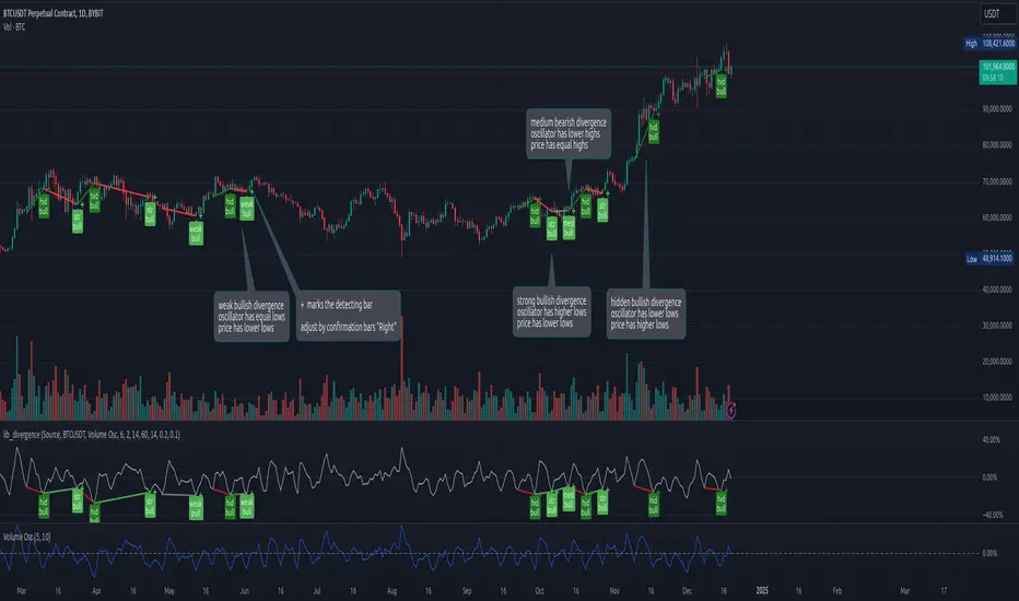
lib_divergenceLibrary "lib_divergence"
offers a commonly usable function to detect divergences. This will take the default RSI or other symbols / indicators / oscillators as source data.
divergence(osc, pivot_left_bars, pivot_right_bars, div_min_range, div_max_range, ref_low, ref_high, min_divergence_offset_fraction, min_divergence_offset_dev_len, min_divergence_offset_atr_mul)
Detects Divergences between Price and Oscillator action. For bullish divergences, look at trend lines between lows. For bearish divergences, look at trend lines between highs. (strong) oscillator trending, price opposing it | (medium) oscillator trending, price trend flat | (weak) price opposite trending, oscillator trend flat | (hidden) price trending, oscillator opposing it. Pivot detection is only properly done in oscillator data, reference price data is only compared at the oscillator pivot (speed optimization)
Parameters:
osc (float) : (series float) oscillator data (can be anything, even another instrument price)
pivot_left_bars (simple int) : (simple int) optional number of bars left of a confirmed pivot point, confirming it is the highest/lowest in the range before and up to the pivot (default: 5)
pivot_right_bars (simple int) : (simple int) optional number of bars right of a confirmed pivot point, confirming it is the highest/lowest in the range from and after the pivot (default: 5)
div_min_range (simple int) : (simple int) optional minimum distance to the pivot point creating a divergence (default: 5)
div_max_range (simple int) : (simple int) optional maximum amount of bars in a divergence (default: 50)
ref_low (float) : (series float) optional reference range to compare the oscillator pivot points to. (default: low)
ref_high (float) : (series float) optional reference range to compare the oscillator pivot points to. (default: high)
min_divergence_offset_fraction (simple float) : (simple float) optional scaling factor for the offset zone (xDeviation) around the last oscillator H/L detecting following equal H/Ls (default: 0.01)
min_divergence_offset_dev_len (simple int) : (simple int) optional lookback distance for the deviation detection for the offset zone around the last oscillator H/L detecting following equal H/Ls. Used as well for the ATR that does the equal H/L detection for the reference price. (default: 14)
min_divergence_offset_atr_mul (simple float) : (simple float) optional scaling factor for the offset zone (xATR) around the last price H/L detecting following equal H/Ls (default: 1)
@return A tuple of deviation flags.
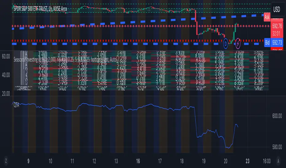
QTALibrary "QTA"
This is simple library for basic Quantitative Technical Analysis for retail investors. One example of it being used can be seen here ().
calculateKellyRatio(returns)
Parameters:
returns (array) : An array of floats representing the returns from bets.
Returns: The calculated Kelly Ratio, which indicates the optimal bet size based on winning and losing probabilities.
calculateAdjustedKellyFraction(kellyRatio, riskTolerance, fedStance)
Parameters:
kellyRatio (float) : The calculated Kelly Ratio.
riskTolerance (float) : A float representing the risk tolerance level.
fedStance (string) : A string indicating the Federal Reserve's stance ("dovish", "hawkish", or neutral).
Returns: The adjusted Kelly Fraction, constrained within the bounds of .
calculateStdDev(returns)
Parameters:
returns (array) : An array of floats representing the returns.
Returns: The standard deviation of the returns, or 0 if insufficient data.
calculateMaxDrawdown(returns)
Parameters:
returns (array) : An array of floats representing the returns.
Returns: The maximum drawdown as a percentage.
calculateEV(avgWinReturn, winProb, avgLossReturn)
Parameters:
avgWinReturn (float) : The average return from winning bets.
winProb (float) : The probability of winning a bet.
avgLossReturn (float) : The average return from losing bets.
Returns: The calculated Expected Value of the bet.
calculateTailRatio(returns)
Parameters:
returns (array) : An array of floats representing the returns.
Returns: The Tail Ratio, or na if the 5th percentile is zero to avoid division by zero.
calculateSharpeRatio(avgReturn, riskFreeRate, stdDev)
Parameters:
avgReturn (float) : The average return of the investment.
riskFreeRate (float) : The risk-free rate of return.
stdDev (float) : The standard deviation of the investment's returns.
Returns: The calculated Sharpe Ratio, or na if standard deviation is zero.
calculateDownsideDeviation(returns)
Parameters:
returns (array) : An array of floats representing the returns.
Returns: The standard deviation of the downside returns, or 0 if no downside returns exist.
calculateSortinoRatio(avgReturn, downsideDeviation)
Parameters:
avgReturn (float) : The average return of the investment.
downsideDeviation (float) : The standard deviation of the downside returns.
Returns: The calculated Sortino Ratio, or na if downside deviation is zero.
calculateVaR(returns, confidenceLevel)
Parameters:
returns (array) : An array of floats representing the returns.
confidenceLevel (float) : A float representing the confidence level (e.g., 0.95 for 95% confidence).
Returns: The Value at Risk at the specified confidence level.
calculateCVaR(returns, varValue)
Parameters:
returns (array) : An array of floats representing the returns.
varValue (float) : The Value at Risk threshold.
Returns: The average Conditional Value at Risk, or na if no returns are below the threshold.
calculateExpectedPriceRange(currentPrice, ev, stdDev, confidenceLevel)
Parameters:
currentPrice (float) : The current price of the asset.
ev (float) : The expected value (in percentage terms).
stdDev (float) : The standard deviation (in percentage terms).
confidenceLevel (float) : The confidence level for the price range (e.g., 1.96 for 95% confidence).
Returns: A tuple containing the minimum and maximum expected prices.
calculateRollingStdDev(returns, window)
Parameters:
returns (array) : An array of floats representing the returns.
window (int) : An integer representing the rolling window size.
Returns: An array of floats representing the rolling standard deviation of returns.
calculateRollingVariance(returns, window)
Parameters:
returns (array) : An array of floats representing the returns.
window (int) : An integer representing the rolling window size.
Returns: An array of floats representing the rolling variance of returns.
calculateRollingMean(returns, window)
Parameters:
returns (array) : An array of floats representing the returns.
window (int) : An integer representing the rolling window size.
Returns: An array of floats representing the rolling mean of returns.
calculateRollingCoefficientOfVariation(returns, window)
Parameters:
returns (array) : An array of floats representing the returns.
window (int) : An integer representing the rolling window size.
Returns: An array of floats representing the rolling coefficient of variation of returns.
calculateRollingSumOfPercentReturns(returns, window)
Parameters:
returns (array) : An array of floats representing the returns.
window (int) : An integer representing the rolling window size.
Returns: An array of floats representing the rolling sum of percent returns.
calculateRollingCumulativeProduct(returns, window)
Parameters:
returns (array) : An array of floats representing the returns.
window (int) : An integer representing the rolling window size.
Returns: An array of floats representing the rolling cumulative product of returns.
calculateRollingCorrelation(priceReturns, volumeReturns, window)
Parameters:
priceReturns (array) : An array of floats representing the price returns.
volumeReturns (array) : An array of floats representing the volume returns.
window (int) : An integer representing the rolling window size.
Returns: An array of floats representing the rolling correlation.
calculateRollingPercentile(returns, window, percentile)
Parameters:
returns (array) : An array of floats representing the returns.
window (int) : An integer representing the rolling window size.
percentile (int) : An integer representing the desired percentile (0-100).
Returns: An array of floats representing the rolling percentile of returns.
calculateRollingMaxMinPercentReturns(returns, window)
Parameters:
returns (array) : An array of floats representing the returns.
window (int) : An integer representing the rolling window size.
Returns: A tuple containing two arrays: rolling max and rolling min percent returns.
calculateRollingPriceToVolumeRatio(price, volData, window)
Parameters:
price (array) : An array of floats representing the price data.
volData (array) : An array of floats representing the volume data.
window (int) : An integer representing the rolling window size.
Returns: An array of floats representing the rolling price-to-volume ratio.
determineMarketRegime(priceChanges)
Parameters:
priceChanges (array) : An array of floats representing the price changes.
Returns: A string indicating the market regime ("Bull", "Bear", or "Neutral").
determineVolatilityRegime(price, window)
Parameters:
price (array) : An array of floats representing the price data.
window (int) : An integer representing the rolling window size.
Returns: An array of floats representing the calculated volatility.
classifyVolatilityRegime(volatility)
Parameters:
volatility (array) : An array of floats representing the calculated volatility.
Returns: A string indicating the volatility regime ("Low" or "High").
method percentPositive(thisArray)
Returns the percentage of positive non-na values in this array.
This method calculates the percentage of positive values in the provided array, ignoring NA values.
Namespace types: array
Parameters:
thisArray (array)
_candleRange()
_PreviousCandleRange(barsback)
Parameters:
barsback (int) : An integer representing how far back you want to get a range
redCandle()
greenCandle()
_WhiteBody()
_BlackBody()
HighOpenDiff()
OpenLowDiff()
_isCloseAbovePreviousOpen(length)
Parameters:
length (int)
_isCloseBelowPrevious()
_isOpenGreaterThanPrevious()
_isOpenLessThanPrevious()
BodyHigh()
BodyLow()
_candleBody()
_BodyAvg(length)
_BodyAvg function.
Parameters:
length (simple int) : Required (recommended is 6).
_SmallBody(length)
Parameters:
length (simple int) : Length of the slow EMA
Returns: a series of bools, after checking if the candle body was less than body average.
_LongBody(length)
Parameters:
length (simple int)
bearWick()
bearWick() function.
Returns: a SERIES of FLOATS, checks if it's a blackBody(open > close), if it is, than check the difference between the high and open, else checks the difference between high and close.
bullWick()
barlength()
sumbarlength()
sumbull()
sumbear()
bull_vol()
bear_vol()
volumeFightMA()
volumeFightDelta()
weightedAVG_BullVolume()
weightedAVG_BearVolume()
VolumeFightDiff()
VolumeFightFlatFilter()
avg_bull_vol(userMA)
avg_bull_vol(int) function.
Parameters:
userMA (int)
avg_bear_vol(userMA)
avg_bear_vol(int) function.
Parameters:
userMA (int)
diff_vol(userMA)
diff_vol(int) function.
Parameters:
userMA (int)
vol_flat(userMA)
vol_flat(int) function.
Parameters:
userMA (int)
_isEngulfingBullish()
_isEngulfingBearish()
dojiup()
dojidown()
EveningStar()
MorningStar()
ShootingStar()
Hammer()
InvertedHammer()
BearishHarami()
BullishHarami()
BullishBelt()
BullishKicker()
BearishKicker()
HangingMan()
DarkCloudCover()
IndicatorsLibrary "Indicators"
cmf(lookback, n_to_smooth)
Calculates the Chaikin's Money Flow.
Parameters:
lookback (simple int)
n_to_smooth (simple int)
Returns: float The Money Flow value.
cmma(lookback, atr_length)
Calculates the CMMA (Close Minus Moving Average) indicator.
Parameters:
lookback (simple int)
atr_length (simple int)
Returns: float The CMMA value.
macd(fast_length, slow_length, n_to_smooth)
Calculates the normalized and scaled MACD.
Parameters:
fast_length (simple int)
slow_length (simple int)
n_to_smooth (simple int)
Returns: A tuple containing .
stochK(length, n_to_smooth)
Calculates a simplified Stochastic Oscillator.
Uses: 100 * ta.sma((close - lowest_low) / (highest_high - lowest_low), n_to_smooth)
Parameters:
length (simple int)
n_to_smooth (simple int)
Returns: float The Stochastic %K value.
williamsR(length)
Calculates the Williams %R using the stochK function.
Uses: -1 * (100 - stoch(length, 1))
Parameters:
length (simple int)
Returns: float The Williams %R value.

lib_kernelLibrary "lib_kernel"
Library "lib_kernel"
This is a tool / library for developers, that contains several common and adapted kernel functions as well as a kernel regression function and enum to easily select and embed a list into the settings dialog.
How to Choose and Modify Kernels in Practice
Compact Support Kernels (e.g., Epanechnikov, Triangular): Use for localized smoothing and emphasizing nearby data.
Oscillatory Kernels (e.g., Wave, Cosine): Ideal for detecting periodic patterns or mean-reverting behavior.
Smooth Tapering Kernels (e.g., Gaussian, Logistic): Use for smoothing long-term trends or identifying global price behavior.
kernel_Epanechnikov(u)
Parameters:
u (float)
kernel_Epanechnikov_alt(u, sensitivity)
Parameters:
u (float)
sensitivity (float)
kernel_Triangular(u)
Parameters:
u (float)
kernel_Triangular_alt(u, sensitivity)
Parameters:
u (float)
sensitivity (float)
kernel_Rectangular(u)
Parameters:
u (float)
kernel_Uniform(u)
Parameters:
u (float)
kernel_Uniform_alt(u, sensitivity)
Parameters:
u (float)
sensitivity (float)
kernel_Logistic(u)
Parameters:
u (float)
kernel_Logistic_alt(u)
Parameters:
u (float)
kernel_Logistic_alt2(u, sigmoid_steepness)
Parameters:
u (float)
sigmoid_steepness (float)
kernel_Gaussian(u)
Parameters:
u (float)
kernel_Gaussian_alt(u, sensitivity)
Parameters:
u (float)
sensitivity (float)
kernel_Silverman(u)
Parameters:
u (float)
kernel_Quartic(u)
Parameters:
u (float)
kernel_Quartic_alt(u, sensitivity)
Parameters:
u (float)
sensitivity (float)
kernel_Biweight(u)
Parameters:
u (float)
kernel_Triweight(u)
Parameters:
u (float)
kernel_Sinc(u)
Parameters:
u (float)
kernel_Wave(u)
Parameters:
u (float)
kernel_Wave_alt(u)
Parameters:
u (float)
kernel_Cosine(u)
Parameters:
u (float)
kernel_Cosine_alt(u, sensitivity)
Parameters:
u (float)
sensitivity (float)
kernel(u, select, alt_modificator)
wrapper for all standard kernel functions, see enum Kernel comments and function descriptions for usage szenarios and parameters
Parameters:
u (float)
select (series Kernel)
alt_modificator (float)
kernel_regression(src, bandwidth, kernel, exponential_distance, alt_modificator)
wrapper for kernel regression with all standard kernel functions, see enum Kernel comments for usage szenarios. performance optimized version using fixed bandwidth and target
Parameters:
src (float) : input data series
bandwidth (simple int) : sample window of nearest neighbours for the kernel to process
kernel (simple Kernel) : type of Kernel to use for processing, see Kernel enum or respective functions for more details
exponential_distance (simple bool) : if true this puts more emphasis on local / more recent values
alt_modificator (float) : see kernel functions for parameter descriptions. Mostly used to pronounce emphasis on local values or introduce a decay/dampening to the kernel output

lib_smcLibrary "lib_smc"
This is an adaptation of LuxAlgo's Smart Money Concepts indicator with numerous changes. Main changes include integration of object based plotting, plenty of performance improvements, live tracking of Order Blocks, integration of volume profiles to refine Order Blocks, and many more.
This is a library for developers, if you want this converted into a working strategy, let me know.
buffer(item, len, force_rotate)
Parameters:
item (float)
len (int)
force_rotate (bool)
buffer(item, len, force_rotate)
Parameters:
item (int)
len (int)
force_rotate (bool)
buffer(item, len, force_rotate)
Parameters:
item (Profile type from robbatt/lib_profile/32)
len (int)
force_rotate (bool)
swings(len)
INTERNAL: detect swing points (HH and LL) in given range
Parameters:
len (simple int) : range to check for new swing points
Returns: values are the price level where and if a new HH or LL was detected, else na
method init(this)
Namespace types: OrderBlockConfig
Parameters:
this (OrderBlockConfig)
method delete(this)
Namespace types: OrderBlock
Parameters:
this (OrderBlock)
method clear_broken(this, broken_buffer)
INTERNAL: delete internal order blocks box coordinates if top/bottom is broken
Namespace types: map
Parameters:
this (map)
broken_buffer (map)
Returns: any_bull_ob_broken, any_bear_ob_broken, broken signals are true if an according order block was broken/mitigated, broken contains the broken block(s)
create_ob(id, mode, start_t, start_i, top, end_t, end_i, bottom, break_price, early_confirmation_price, config, init_plot, force_overlay)
INTERNAL: set internal order block coordinates
Parameters:
id (int)
mode (int) : 1: bullish, -1 bearish block
start_t (int)
start_i (int)
top (float)
end_t (int)
end_i (int)
bottom (float)
break_price (float)
early_confirmation_price (float)
config (OrderBlockConfig)
init_plot (bool)
force_overlay (bool)
Returns: signals are true if an according order block was broken/mitigated
method align_to_profile(block, align_edge, align_break_price)
Namespace types: OrderBlock
Parameters:
block (OrderBlock)
align_edge (bool)
align_break_price (bool)
method create_profile(block, opens, tops, bottoms, closes, values, resolution, vah_pc, val_pc, args, init_calculated, init_plot, force_overlay)
Namespace types: OrderBlock
Parameters:
block (OrderBlock)
opens (array)
tops (array)
bottoms (array)
closes (array)
values (array)
resolution (int)
vah_pc (float)
val_pc (float)
args (ProfileArgs type from robbatt/lib_profile/32)
init_calculated (bool)
init_plot (bool)
force_overlay (bool)
method create_profile(block, resolution, vah_pc, val_pc, args, init_calculated, init_plot, force_overlay)
Namespace types: OrderBlock
Parameters:
block (OrderBlock)
resolution (int)
vah_pc (float)
val_pc (float)
args (ProfileArgs type from robbatt/lib_profile/32)
init_calculated (bool)
init_plot (bool)
force_overlay (bool)
track_obs(swing_len, hh, ll, top, btm, bull_bos_alert, bull_choch_alert, bear_bos_alert, bear_choch_alert, min_block_size, max_block_size, config_bull, config_bear, init_plot, force_overlay, enabled, extend_blocks, clear_broken_buffer_before, align_edge_to_value_area, align_break_price_to_poc, profile_args_bull, profile_args_bear, use_soft_confirm, soft_confirm_offset, use_retracements_with_FVG_out)
Parameters:
swing_len (int)
hh (float)
ll (float)
top (float)
btm (float)
bull_bos_alert (bool)
bull_choch_alert (bool)
bear_bos_alert (bool)
bear_choch_alert (bool)
min_block_size (float)
max_block_size (float)
config_bull (OrderBlockConfig)
config_bear (OrderBlockConfig)
init_plot (bool)
force_overlay (bool)
enabled (bool)
extend_blocks (simple bool)
clear_broken_buffer_before (simple bool)
align_edge_to_value_area (simple bool)
align_break_price_to_poc (simple bool)
profile_args_bull (ProfileArgs type from robbatt/lib_profile/32)
profile_args_bear (ProfileArgs type from robbatt/lib_profile/32)
use_soft_confirm (simple bool)
soft_confirm_offset (float)
use_retracements_with_FVG_out (simple bool)
method draw(this, config, extend_only)
Namespace types: OrderBlock
Parameters:
this (OrderBlock)
config (OrderBlockConfig)
extend_only (bool)
method draw(blocks, config)
INTERNAL: plot order blocks
Namespace types: array
Parameters:
blocks (array)
config (OrderBlockConfig)
method draw(blocks, config)
INTERNAL: plot order blocks
Namespace types: map
Parameters:
blocks (map)
config (OrderBlockConfig)
method cleanup(this, ob_bull, ob_bear)
removes all Profiles that are older than the latest OrderBlock from this profile buffer
Namespace types: array
Parameters:
this (array type from robbatt/lib_profile/32)
ob_bull (OrderBlock)
ob_bear (OrderBlock)
_plot_swing_points(mode, x, y, show_swing_points, linecolor_swings, keep_history, show_latest_swings_levels, trail_x, trail_y, trend)
INTERNAL: plot swing points
Parameters:
mode (int) : 1: bullish, -1 bearish block
x (int) : x-coordingate of swing point to plot (bar_index)
y (float) : y-coordingate of swing point to plot (price)
show_swing_points (bool) : switch to enable/disable plotting of swing point labels
linecolor_swings (color) : color for swing point labels and lates level lines
keep_history (bool) : weater to remove older swing point labels and only keep the most recent
show_latest_swings_levels (bool)
trail_x (int) : x-coordinate for latest swing point (bar_index)
trail_y (float) : y-coordinate for latest swing point (price)
trend (int) : the current trend 1: bullish, -1: bearish, to determine Strong/Weak Low/Highs
_pivot_lvl(mode, trend, hhll_x, hhll, super_hhll, filter_insignificant_internal_breaks)
INTERNAL: detect whether a structural level has been broken and if it was in trend direction (BoS) or against trend direction (ChoCh), also track the latest high and low swing points
Parameters:
mode (simple int) : detect 1: bullish, -1 bearish pivot points
trend (int) : current trend direction
hhll_x (int) : x-coordinate of newly detected hh/ll (bar_index)
hhll (float) : y-coordinate of newly detected hh/ll (price)
super_hhll (float) : level/y-coordinate of superior hhll (if this is an internal structure pivot level)
filter_insignificant_internal_breaks (bool) : if true pivot points / internal structure will be ignored where the wick in trend direction is longer than the opposite (likely to push further in direction of main trend)
Returns: coordinates of internal structure that has been broken (x,y): start of structure, (trail_x, trail_y): tracking hh/ll after structure break, (bos_alert, choch_alert): signal whether a structural level has been broken
_plot_structure(x, y, is_bos, is_choch, line_color, line_style, label_style, label_size, keep_history)
INTERNAL: plot structural breaks (BoS/ChoCh)
Parameters:
x (int) : x-coordinate of newly broken structure (bar_index)
y (float) : y-coordinate of newly broken structure (price)
is_bos (bool) : whether this structural break was in trend direction
is_choch (bool) : whether this structural break was against trend direction
line_color (color) : color for the line connecting the structural level and the breaking candle
line_style (string) : style (line.style_dashed/solid) for the line connecting the structural level and the breaking candle
label_style (string) : style (label.style_label_down/up) for the label above/below the line connecting the structural level and the breaking candle
label_size (string) : size (size.small/tiny) for the label above/below the line connecting the structural level and the breaking candle
keep_history (bool) : weater to remove older swing point labels and only keep the most recent
structure_values(length, super_hh, super_ll, filter_insignificant_internal_breaks)
detect (and plot) structural breaks and the resulting new trend
Parameters:
length (simple int) : lookback period for swing point detection
super_hh (float) : level/y-coordinate of superior hh (for internal structure detection)
super_ll (float) : level/y-coordinate of superior ll (for internal structure detection)
filter_insignificant_internal_breaks (bool) : if true pivot points / internal structure will be ignored where the wick in trend direction is longer than the opposite (likely to push further in direction of main trend)
Returns: trend: direction 1:bullish -1:bearish, (bull_bos_alert, bull_choch_alert, top_x, top_y, trail_up_x, trail_up): whether and which level broke in a bullish direction, trailing high, (bbear_bos_alert, bear_choch_alert, tm_x, btm_y, trail_dn_x, trail_dn): same in bearish direction
structure_plot(trend, bull_bos_alert, bull_choch_alert, top_x, top_y, trail_up_x, trail_up, hh, bear_bos_alert, bear_choch_alert, btm_x, btm_y, trail_dn_x, trail_dn, ll, color_bull, color_bear, show_swing_points, show_latest_swings_levels, show_bos, show_choch, line_style, label_size, keep_history)
detect (and plot) structural breaks and the resulting new trend
Parameters:
trend (int) : crrent trend 1: bullish, -1: bearish
bull_bos_alert (bool) : if there was a bullish bos alert -> plot it
bull_choch_alert (bool) : if there was a bullish choch alert -> plot it
top_x (int) : latest shwing high x
top_y (float) : latest swing high y
trail_up_x (int) : trailing high x
trail_up (float) : trailing high y
hh (float) : if there was a higher high
bear_bos_alert (bool) : if there was a bearish bos alert -> plot it
bear_choch_alert (bool) : if there was a bearish chock alert -> plot it
btm_x (int) : latest swing low x
btm_y (float) : latest swing low y
trail_dn_x (int) : trailing low x
trail_dn (float) : trailing low y
ll (float) : if there was a lower low
color_bull (color) : color for bullish BoS/ChoCh levels
color_bear (color) : color for bearish BoS/ChoCh levels
show_swing_points (bool) : whether to plot swing point labels
show_latest_swings_levels (bool) : whether to track and plot latest swing point levels with lines
show_bos (bool) : whether to plot BoS levels
show_choch (bool) : whether to plot ChoCh levels
line_style (string) : whether to plot BoS levels
label_size (string) : label size of plotted BoS/ChoCh levels
keep_history (bool) : weater to remove older swing point labels and only keep the most recent
structure(length, color_bull, color_bear, super_hh, super_ll, filter_insignificant_internal_breaks, show_swing_points, show_latest_swings_levels, show_bos, show_choch, line_style, label_size, keep_history, enabled)
detect (and plot) structural breaks and the resulting new trend
Parameters:
length (simple int) : lookback period for swing point detection
color_bull (color) : color for bullish BoS/ChoCh levels
color_bear (color) : color for bearish BoS/ChoCh levels
super_hh (float) : level/y-coordinate of superior hh (for internal structure detection)
super_ll (float) : level/y-coordinate of superior ll (for internal structure detection)
filter_insignificant_internal_breaks (bool) : if true pivot points / internal structure will be ignored where the wick in trend direction is longer than the opposite (likely to push further in direction of main trend)
show_swing_points (bool) : whether to plot swing point labels
show_latest_swings_levels (bool) : whether to track and plot latest swing point levels with lines
show_bos (bool) : whether to plot BoS levels
show_choch (bool) : whether to plot ChoCh levels
line_style (string) : whether to plot BoS levels
label_size (string) : label size of plotted BoS/ChoCh levels
keep_history (bool) : weater to remove older swing point labels and only keep the most recent
enabled (bool)
_check_equal_level(mode, len, eq_threshold, enabled)
INTERNAL: detect equal levels (double top/bottom)
Parameters:
mode (int) : detect 1: bullish/high, -1 bearish/low pivot points
len (int) : lookback period for equal level (swing point) detection
eq_threshold (float) : maximum price offset for a level to be considered equal
enabled (bool)
Returns: eq_alert whether an equal level was detected and coordinates of the first and the second level/swing point
_plot_equal_level(show_eq, x1, y1, x2, y2, label_txt, label_style, label_size, line_color, line_style, keep_history)
INTERNAL: plot equal levels (double top/bottom)
Parameters:
show_eq (bool) : whether to plot the level or not
x1 (int) : x-coordinate of the first level / swing point
y1 (float) : y-coordinate of the first level / swing point
x2 (int) : x-coordinate of the second level / swing point
y2 (float) : y-coordinate of the second level / swing point
label_txt (string) : text for the label above/below the line connecting the equal levels
label_style (string) : style (label.style_label_down/up) for the label above/below the line connecting the equal levels
label_size (string) : size (size.tiny) for the label above/below the line connecting the equal levels
line_color (color) : color for the line connecting the equal levels (and it's label)
line_style (string) : style (line.style_dotted) for the line connecting the equal levels
keep_history (bool) : weater to remove older swing point labels and only keep the most recent
equal_levels_values(len, threshold, enabled)
detect (and plot) equal levels (double top/bottom), returns coordinates
Parameters:
len (int) : lookback period for equal level (swing point) detection
threshold (float) : maximum price offset for a level to be considered equal
enabled (bool) : whether detection is enabled
Returns: (eqh_alert, eqh_x1, eqh_y1, eqh_x2, eqh_y2) whether an equal high was detected and coordinates of the first and the second level/swing point, (eql_alert, eql_x1, eql_y1, eql_x2, eql_y2) same for equal lows
equal_levels_plot(eqh_x1, eqh_y1, eqh_x2, eqh_y2, eql_x1, eql_y1, eql_x2, eql_y2, color_eqh, color_eql, show, keep_history)
detect (and plot) equal levels (double top/bottom), returns coordinates
Parameters:
eqh_x1 (int) : coordinates of first point of equal high
eqh_y1 (float) : coordinates of first point of equal high
eqh_x2 (int) : coordinates of second point of equal high
eqh_y2 (float) : coordinates of second point of equal high
eql_x1 (int) : coordinates of first point of equal low
eql_y1 (float) : coordinates of first point of equal low
eql_x2 (int) : coordinates of second point of equal low
eql_y2 (float) : coordinates of second point of equal low
color_eqh (color) : color for the line connecting the equal highs (and it's label)
color_eql (color) : color for the line connecting the equal lows (and it's label)
show (bool) : whether plotting is enabled
keep_history (bool) : weater to remove older swing point labels and only keep the most recent
Returns: (eqh_alert, eqh_x1, eqh_y1, eqh_x2, eqh_y2) whether an equal high was detected and coordinates of the first and the second level/swing point, (eql_alert, eql_x1, eql_y1, eql_x2, eql_y2) same for equal lows
equal_levels(len, threshold, color_eqh, color_eql, enabled, show, keep_history)
detect (and plot) equal levels (double top/bottom)
Parameters:
len (int) : lookback period for equal level (swing point) detection
threshold (float) : maximum price offset for a level to be considered equal
color_eqh (color) : color for the line connecting the equal highs (and it's label)
color_eql (color) : color for the line connecting the equal lows (and it's label)
enabled (bool) : whether detection is enabled
show (bool) : whether plotting is enabled
keep_history (bool) : weater to remove older swing point labels and only keep the most recent
Returns: (eqh_alert) whether an equal high was detected, (eql_alert) same for equal lows
_detect_fvg(mode, enabled, o, h, l, c, filter_insignificant_fvgs, change_tf)
INTERNAL: detect FVG (fair value gap)
Parameters:
mode (int) : detect 1: bullish, -1 bearish gaps
enabled (bool) : whether detection is enabled
o (float) : reference source open
h (float) : reference source high
l (float) : reference source low
c (float) : reference source close
filter_insignificant_fvgs (bool) : whether to calculate and filter small/insignificant gaps
change_tf (bool) : signal when the previous reference timeframe closed, triggers new calculation
Returns: whether a new FVG was detected and its top/mid/bottom levels
_clear_broken_fvg(mode, upper_boxes, lower_boxes)
INTERNAL: clear mitigated FVGs (fair value gaps)
Parameters:
mode (int) : detect 1: bullish, -1 bearish gaps
upper_boxes (array) : array that stores the upper parts of the FVG boxes
lower_boxes (array) : array that stores the lower parts of the FVG boxes
_plot_fvg(mode, show, top, mid, btm, border_color, extend_box)
INTERNAL: plot (and clear broken) FVG (fair value gap)
Parameters:
mode (int) : plot 1: bullish, -1 bearish gap
show (bool) : whether plotting is enabled
top (float) : top level of fvg
mid (float) : center level of fvg
btm (float) : bottom level of fvg
border_color (color) : color for the FVG box
extend_box (int) : how many bars into the future the FVG box should be extended after detection
fvgs_values(o, h, l, c, filter_insignificant_fvgs, change_tf, enabled)
detect (and plot / clear broken) FVGs (fair value gaps), and return alerts and level values
Parameters:
o (float) : reference source open
h (float) : reference source high
l (float) : reference source low
c (float) : reference source close
filter_insignificant_fvgs (bool) : whether to calculate and filter small/insignificant gaps
change_tf (bool) : signal when the previous reference timeframe closed, triggers new calculation
enabled (bool) : whether detection is enabled
Returns: (bullish_fvg_alert, bull_top, bull_mid, bull_btm): whether a new bullish FVG was detected and its top/mid/bottom levels, (bearish_fvg_alert, bear_top, bear_mid, bear_btm): same for bearish FVGs
fvgs_plot(bullish_fvg_alert, bull_top, bull_mid, bull_btm, bearish_fvg_alert, bear_top, bear_mid, bear_btm, color_bull, color_bear, extend_box, show)
Parameters:
bullish_fvg_alert (bool)
bull_top (float)
bull_mid (float)
bull_btm (float)
bearish_fvg_alert (bool)
bear_top (float)
bear_mid (float)
bear_btm (float)
color_bull (color) : color for bullish FVG boxes
color_bear (color) : color for bearish FVG boxes
extend_box (int) : how many bars into the future the FVG box should be extended after detection
show (bool) : whether plotting is enabled
Returns: (bullish_fvg_alert, bull_top, bull_mid, bull_btm): whether a new bullish FVG was detected and its top/mid/bottom levels, (bearish_fvg_alert, bear_top, bear_mid, bear_btm): same for bearish FVGs
fvgs(o, h, l, c, filter_insignificant_fvgs, change_tf, color_bull, color_bear, extend_box, enabled, show)
detect (and plot / clear broken) FVGs (fair value gaps)
Parameters:
o (float) : reference source open
h (float) : reference source high
l (float) : reference source low
c (float) : reference source close
filter_insignificant_fvgs (bool) : whether to calculate and filter small/insignificant gaps
change_tf (bool) : signal when the previous reference timeframe closed, triggers new calculation
color_bull (color) : color for bullish FVG boxes
color_bear (color) : color for bearish FVG boxes
extend_box (int) : how many bars into the future the FVG box should be extended after detection
enabled (bool) : whether detection is enabled
show (bool) : whether plotting is enabled
Returns: (bullish_fvg_alert): whether a new bullish FVG was detected, (bearish_fvg_alert): same for bearish FVGs
OrderBlock
Fields:
id (series int)
dir (series int)
left_top (chart.point)
right_bottom (chart.point)
break_price (series float)
early_confirmation_price (series float)
ltf_high (array)
ltf_low (array)
ltf_volume (array)
plot (Box type from robbatt/lib_plot_objects/49)
profile (Profile type from robbatt/lib_profile/32)
trailing (series bool)
extending (series bool)
awaiting_confirmation (series bool)
touched_break_price_before_confirmation (series bool)
soft_confirmed (series bool)
has_fvg_out (series bool)
hidden (series bool)
broken (series bool)
OrderBlockConfig
Fields:
show (series bool)
show_last (series int)
show_id (series bool)
show_profile (series bool)
args (BoxArgs type from robbatt/lib_plot_objects/49)
txt (series string)
txt_args (BoxTextArgs type from robbatt/lib_plot_objects/49)
delete_when_broken (series bool)
broken_args (BoxArgs type from robbatt/lib_plot_objects/49)
broken_txt (series string)
broken_txt_args (BoxTextArgs type from robbatt/lib_plot_objects/49)
broken_profile_args (ProfileArgs type from robbatt/lib_profile/32)
use_profile (series bool)
profile_args (ProfileArgs type from robbatt/lib_profile/32)
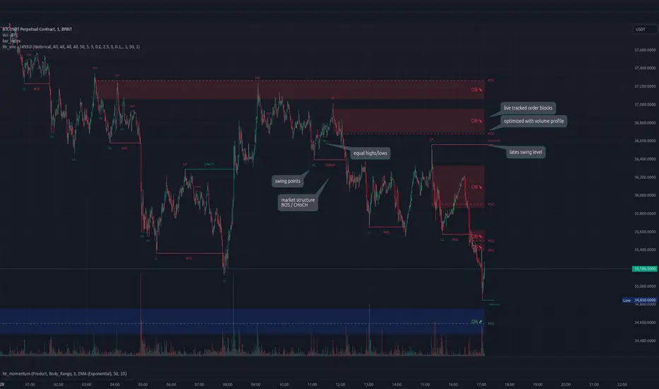
FibRatiosLibrary "FibRatios"
Library with calculation logic for fib retracement, extension and ratios
retracement(a, b, ratio, logScale, precision)
Calculates the retracement for points a, b with given ratio and scale
Parameters:
a (float) : Starting point a
b (float) : Second point b
ratio (float) : Ratio for which we need to calculate retracement c
logScale (bool) : Flag to get calculations in log scale. Default is false
precision (int) : rounding precision. If set to netagive number, round_to_mintick is applied. Default is -1
Returns: retracement point c for points a,b with given ratio and scale
retracementRatio(a, b, c, logScale, precision)
Calculates the retracement ratio for points a, b, c with given scale
Parameters:
a (float) : Starting point a
b (float) : Second point b
c (float) : Retracement point. c should be placed between a and b
logScale (bool) : Flag to get calculations in log scale. Default is false
precision (int) : rounding precision. If set to netagive number, round_to_mintick is applied. Default is 3
Returns: retracement ratio for points a,b,c on given scale
extension(a, b, c, ratio, logScale, precision)
Calculates the extensions for points a, b, c with given ratio and scale
Parameters:
a (float) : Starting point a
b (float) : Second point b
c (float) : Retracement point. c should be placed between a and b
ratio (float) : Ratio for which we need to calculate extension d
logScale (bool) : Flag to get calculations in log scale. Default is false
precision (int) : rounding precision. If set to netagive number, round_to_mintick is applied. Default is -1
Returns: extensoin point d for points a,b,c with given ratio and scale
extensionRatio(a, b, c, d, logScale, precision)
Calculates the extension ratio for points a, b, c, d with given scale
Parameters:
a (float) : Starting point a
b (float) : Second point b
c (float) : Retracement point. c should be placed between a and b
d (float) : Extension point. d should be placed beyond a, c. But, can be with b,c or beyond b
logScale (bool) : Flag to get calculations in log scale. Default is false
precision (int) : rounding precision. If set to netagive number, round_to_mintick is applied. Default is 3
Returns: extension ratio for points a,b,c,d on given scale

MathHelpersLibrary "MathHelpers"
Overview
A collection of helper functions for designing indicators and strategies.
calculateATR(length, log)
Calculates the Average True Range (ATR) or Log ATR based on the 'log' parameter. Sans Wilder's Smoothing
Parameters:
length (simple int)
log (simple bool)
Returns: float The calculated ATR value. Returns Log ATR if `log` is true, otherwise returns standard ATR.
CDF(z)
Computes the Cumulative Distribution Function (CDF) for a given value 'z', mimicking the CDF function in "Statistically Sound Indicators" by Timothy Masters.
Parameters:
z (simple float)
Returns: float The CDF value corresponding to the input `z`, ranging between 0 and 1.
logReturns(lookback)
Calculates the logarithmic returns over a specified lookback period.
Parameters:
lookback (simple int)
Returns: float The calculated logarithmic return. Returns `na` if insufficient data is available.
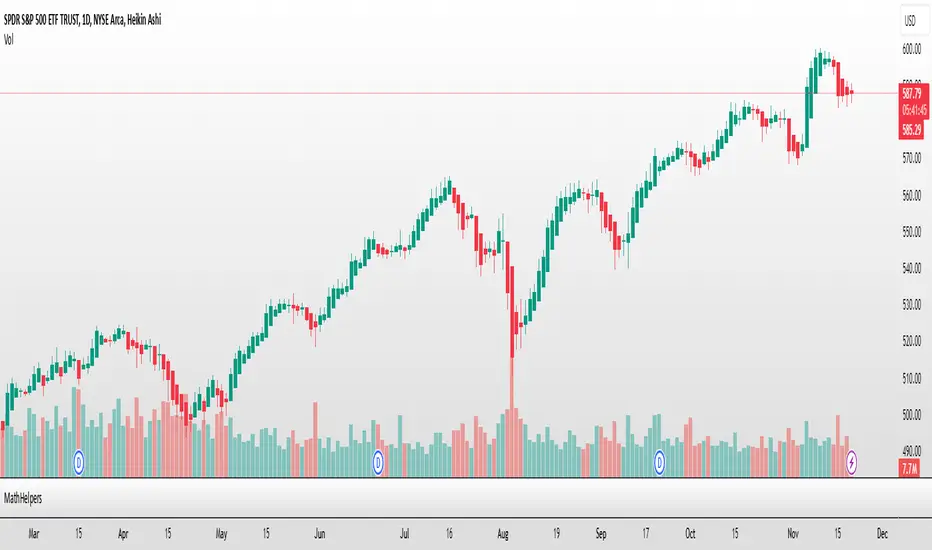
lib_momentumLibrary "lib_momentum"
This library calculates the momentum, derived from a sample range of prior candles. Depending on set MomentumType it either deduces the momentum from the price, volume, or a product of both. If price/product are selected, you can choose from SampleType if only candle body, full range from high to low or a combination of both (body counts full, wicks half for each direction) should be used. Optional: You can choose to normalize the results, dividing each value by its average (normalization_ma_length, normalization_ma). This will allow comparison between different instruments. For the normalization Moving Average you can choose any currently supported in my lib_no_delay.
get_momentum(momentum_type, sample_type, sample_length, normalization_ma_length, normalization_ma)
Parameters:
momentum_type (series MomentumType) : select one of MomentumType. to sample the price, volume or a product of both
sample_type (series SampleType) : select one of SampleType. to sample the body, total range from high to low or a combination of both (body count full, wicks half for each direction)
sample_length (simple int) : how many candles should be sampled (including the current)
normalization_ma_length (simple int) : if you want to normalize results (momentum / momentum average) this sets the period for the average. (default = 0 => no normalization)
normalization_ma (simple MovingAverage enum from robbatt/lib_no_delay/9) : is the type of moving average to normalize / compare with
Returns: returns the current momentum where the total line is not just (up - down) but also sampled over the sample_length and can therefore be used as trend indicator. If up/down fail to reach total's level it's a sign of decreasing momentum, if up/down exceed total the trend it's a sign of increasing momentum.
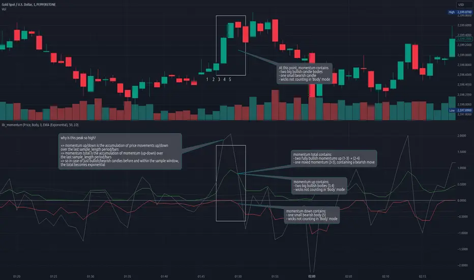
analytics_tablesLibrary "analytics_tables"
📝 Description
This library provides the implementation of several performance-related statistics and metrics, presented in the form of tables.
The metrics shown in the afforementioned tables where developed during the past years of my in-depth analalysis of various strategies in an atempt to reason about the performance of each strategy.
The visualization and some statistics where inspired by the existing implementations of the "Seasonality" script, and the performance matrix implementations of @QuantNomad and @ZenAndTheArtOfTrading scripts.
While this library is meant to be used by my strategy framework "Template Trailing Strategy (Backtester)" script, I wrapped it in a library hoping this can be usefull for other community strategy scripts that will be released in the future.
🤔 How to Guide
To use the functionality this library provides in your script you have to import it first!
Copy the import statement of the latest release by pressing the copy button below and then paste it into your script. Give a short name to this library so you can refer to it later on. The import statement should look like this:
import jason5480/analytics_tables/1 as ant
There are three types of tables provided by this library in the initial release. The stats table the metrics table and the seasonality table.
Each one shows different kinds of performance statistics.
The table UDT shall be initialized once using the `init()` method.
They can be updated using the `update()` method where the updated data UDT object shall be passed.
The data UDT can also initialized and get updated on demend depending on the use case
A code example for the StatsTable is the following:
var ant.StatsData statsData = ant.StatsData.new()
statsData.update(SideStats.new(), SideStats.new(), 0)
if (barstate.islastconfirmedhistory or (barstate.isrealtime and barstate.isconfirmed))
var statsTable = ant.StatsTable.new().init(ant.getTablePos('TOP', 'RIGHT'))
statsTable.update(statsData)
A code example for the MetricsTable is the following:
var ant.StatsData statsData = ant.StatsData.new()
statsData.update(ant.SideStats.new(), ant.SideStats.new(), 0)
if (barstate.islastconfirmedhistory or (barstate.isrealtime and barstate.isconfirmed))
var metricsTable = ant.MetricsTable.new().init(ant.getTablePos('BOTTOM', 'RIGHT'))
metricsTable.update(statsData, 10)
A code example for the SeasonalityTable is the following:
var ant.SeasonalData seasonalData = ant.SeasonalData.new().init(Seasonality.monthOfYear)
seasonalData.update()
if (barstate.islastconfirmedhistory or (barstate.isrealtime and barstate.isconfirmed))
var seasonalTable = ant.SeasonalTable.new().init(seasonalData, ant.getTablePos('BOTTOM', 'LEFT'))
seasonalTable.update(seasonalData)
🏋️♂️ Please refer to the "EXAMPLE" regions of the script for more advanced and up to date code examples!
Special thanks to @Mrcrbw for the proposal to develop this library and @DCNeu for the constructive feedback 🏆.
getTablePos(ypos, xpos)
Get table position compatible string
Parameters:
ypos (simple string) : The position on y axise
xpos (simple string) : The position on x axise
Returns: The position to be passed to the table
method init(this, pos, height, width, positiveTxtColor, negativeTxtColor, neutralTxtColor, positiveBgColor, negativeBgColor, neutralBgColor)
Initialize the stats table object with the given colors in the given position
Namespace types: StatsTable
Parameters:
this (StatsTable) : The stats table object
pos (simple string) : The table position string
height (simple float) : The height of the table as a percentage of the charts height. By default, 0 auto-adjusts the height based on the text inside the cells
width (simple float) : The width of the table as a percentage of the charts height. By default, 0 auto-adjusts the width based on the text inside the cells
positiveTxtColor (simple color) : The text color when positive
negativeTxtColor (simple color) : The text color when negative
neutralTxtColor (simple color) : The text color when neutral
positiveBgColor (simple color) : The background color with transparency when positive
negativeBgColor (simple color) : The background color with transparency when negative
neutralBgColor (simple color) : The background color with transparency when neutral
method init(this, pos, height, width, neutralBgColor)
Initialize the metrics table object with the given colors in the given position
Namespace types: MetricsTable
Parameters:
this (MetricsTable) : The metrics table object
pos (simple string) : The table position string
height (simple float) : The height of the table as a percentage of the charts height. By default, 0 auto-adjusts the height based on the text inside the cells
width (simple float) : The width of the table as a percentage of the charts width. By default, 0 auto-adjusts the width based on the text inside the cells
neutralBgColor (simple color) : The background color with transparency when neutral
method init(this, seas)
Initialize the seasonal data
Namespace types: SeasonalData
Parameters:
this (SeasonalData) : The seasonal data object
seas (simple Seasonality) : The seasonality of the matrix data
method init(this, data, pos, maxNumOfYears, height, width, extended, neutralTxtColor, neutralBgColor)
Initialize the seasonal table object with the given colors in the given position
Namespace types: SeasonalTable
Parameters:
this (SeasonalTable) : The seasonal table object
data (SeasonalData) : The seasonality data of the table
pos (simple string) : The table position string
maxNumOfYears (simple int) : The maximum number of years that fit into the table
height (simple float) : The height of the table as a percentage of the charts height. By default, 0 auto-adjusts the height based on the text inside the cells
width (simple float) : The width of the table as a percentage of the charts width. By default, 0 auto-adjusts the width based on the text inside the cells
extended (simple bool) : The seasonal table with extended columns for performance
neutralTxtColor (simple color) : The text color when neutral
neutralBgColor (simple color) : The background color with transparency when neutral
method update(this, wins, losses, numOfInconclusiveExits)
Update the strategy info data of the strategy
Namespace types: StatsData
Parameters:
this (StatsData) : The strategy statistics object
wins (SideStats)
losses (SideStats)
numOfInconclusiveExits (int) : The number of inconclusive trades
method update(this, stats, positiveTxtColor, negativeTxtColor, negativeBgColor, neutralBgColor)
Update the stats table object with the given data
Namespace types: StatsTable
Parameters:
this (StatsTable) : The stats table object
stats (StatsData) : The stats data to update the table
positiveTxtColor (simple color) : The text color when positive
negativeTxtColor (simple color) : The text color when negative
negativeBgColor (simple color) : The background color with transparency when negative
neutralBgColor (simple color) : The background color with transparency when neutral
method update(this, stats, buyAndHoldPerc, positiveTxtColor, negativeTxtColor, positiveBgColor, negativeBgColor)
Update the metrics table object with the given data
Namespace types: MetricsTable
Parameters:
this (MetricsTable) : The metrics table object
stats (StatsData) : The stats data to update the table
buyAndHoldPerc (float) : The buy and hold percetage
positiveTxtColor (simple color) : The text color when positive
negativeTxtColor (simple color) : The text color when negative
positiveBgColor (simple color) : The background color with transparency when positive
negativeBgColor (simple color) : The background color with transparency when negative
method update(this)
Update the seasonal data based on the season and eon timeframe
Namespace types: SeasonalData
Parameters:
this (SeasonalData) : The seasonal data object
method update(this, data, positiveTxtColor, negativeTxtColor, neutralTxtColor, positiveBgColor, negativeBgColor, neutralBgColor, timeBgColor)
Update the seasonal table object with the given data
Namespace types: SeasonalTable
Parameters:
this (SeasonalTable) : The seasonal table object
data (SeasonalData) : The seasonal cell data to update the table
positiveTxtColor (simple color) : The text color when positive
negativeTxtColor (simple color) : The text color when negative
neutralTxtColor (simple color) : The text color when neutral
positiveBgColor (simple color) : The background color with transparency when positive
negativeBgColor (simple color) : The background color with transparency when negative
neutralBgColor (simple color) : The background color with transparency when neutral
timeBgColor (simple color) : The background color of the time gradient
SideStats
Object that represents the strategy statistics data of one side win or lose
Fields:
numOf (series int)
sumFreeProfit (series float)
freeProfitStDev (series float)
sumProfit (series float)
profitStDev (series float)
sumGain (series float)
gainStDev (series float)
avgQuantityPerc (series float)
avgCapitalRiskPerc (series float)
avgTPExecutedCount (series float)
avgRiskRewardRatio (series float)
maxStreak (series int)
StatsTable
Object that represents the stats table
Fields:
table (series table) : The actual table
rows (series int) : The number of rows of the table
columns (series int) : The number of columns of the table
StatsData
Object that represents the statistics data of the strategy
Fields:
wins (SideStats)
losses (SideStats)
numOfInconclusiveExits (series int)
avgFreeProfitStr (series string)
freeProfitStDevStr (series string)
lossFreeProfitStDevStr (series string)
avgProfitStr (series string)
profitStDevStr (series string)
lossProfitStDevStr (series string)
avgQuantityStr (series string)
MetricsTable
Object that represents the metrics table
Fields:
table (series table) : The actual table
rows (series int) : The number of rows of the table
columns (series int) : The number of columns of the table
SeasonalData
Object that represents the seasonal table dynamic data
Fields:
seasonality (series Seasonality)
eonToMatrixRow (map)
numOfEons (series int)
mostRecentMatrixRow (series int)
balances (matrix)
returnPercs (matrix)
maxDDs (matrix)
eonReturnPercs (array)
eonCAGRs (array)
eonMaxDDs (array)
SeasonalTable
Object that represents the seasonal table
Fields:
table (series table) : The actual table
headRows (series int) : The number of head rows of the table
headColumns (series int) : The number of head columns of the table
eonRows (series int) : The number of eon rows of the table
seasonColumns (series int) : The number of season columns of the table
statsRows (series int)
statsColumns (series int) : The number of stats columns of the table
rows (series int) : The number of rows of the table
columns (series int) : The number of columns of the table
extended (series bool) : Whether the table has additional performance statistics

BinaryInsertionSortLibrary "BinaryInsertionSort"
Library containing functions which can help create sorted array based on binary insertion sort.
This sorting will be quicker than array.sort function if the sorting needs to be done on every bar and the size of the array is comparatively big.
method binary_search_basic(sortedArray, item, order)
binary_search_basic - finds the closest index of the value
Namespace types: array
Parameters:
sortedArray (array) : array which is assumed to be sorted in the requested order
item (float) : float item which needs to be searched in the sorted array
order (int) : Sort order - positive number means ascending order whereas negative number represents descending order
Returns: int index at which the item can be inserted into sorted array
method binary_search_basic(sortedArray, item, order)
binary_search_basic - finds the closest index of the value
Namespace types: array
Parameters:
sortedArray (array) : array which is assumed to be sorted in the requested order
item (int) : int item which needs to be searched in the sorted array
order (int) : Sort order - positive number means ascending order whereas negative number represents descending order
Returns: int index at which the item can be inserted into sorted array
method binary_insertion_sort(sortedArray, item, order)
binary insertion sort - inserts item into sorted array while maintaining sort order
Namespace types: array
Parameters:
sortedArray (array) : array which is assumed to be sorted in the requested order
item (float) : float item which needs to be inserted into sorted array
order (int) : Sort order - positive number means ascending order whereas negative number represents descending order
Returns: int index at which the item is inserted into sorted array
method binary_insertion_sort(sortedArray, item, order)
binary insertion sort - inserts item into sorted array while maintaining sort order
Namespace types: array
Parameters:
sortedArray (array) : array which is assumed to be sorted in the requested order
item (int) : int item which needs to be inserted into sorted array
order (int) : Sort order - positive number means ascending order whereas negative number represents descending order
Returns: int index at which the item is inserted into sorted array
update_sort_indices(sortIndices, newItemIndex)
adds the sort index of new item added to sorted array and also updates existing sort indices.
Parameters:
sortIndices (array) : array containing sort indices of an array.
newItemIndex (int) : sort index of new item added to sorted array
Returns: void
get_array_of_series(item, order)
Converts series into array and sorted array.
Parameters:
item (float) : float series
order (int) : Sort order - positive number means ascending order whereas negative number represents descending order
Returns:
get_array_of_series(item, order)
Converts series into array and sorted array.
Parameters:
item (int) : int series
order (int) : Sort order - positive number means ascending order whereas negative number represents descending order
Returns:
get_sorted_arrays(item, order)
Converts series into array and sorted array. Also calculates the sort order of the value array
Parameters:
item (float) : float|int series
order (int) : Sort order - positive number means ascending order whereas negative number represents descending order
Returns:
get_sorted_arrays(item, order)
Converts series into array and sorted array. Also calculates the sort order of the value array
Parameters:
item (int) : int series
order (int) : Sort order - positive number means ascending order whereas negative number represents descending order
Returns:
lib_no_delayLibrary "lib_no_delay"
This library contains modifications to standard functions that return na before reaching the bar of their 'length' parameter.
That is because they do not compromise speed at current time for correct results in the past. This is good for live trading in short timeframes but killing applications on Monthly / Weekly timeframes if instruments, like in crypto, do not have extensive history (why would you even trade the monthly on a meme coin ... not my decision).
Also, some functions rely on source (value at previous bar), which is not available on bar 1 and therefore cascading to a na value up to the last bar ... which in turn leads to a non displaying indicator and waste of time debugging this)
Anyway ... there you go, let me know if I should add more functions.
sma(source, length)
Parameters:
source (float) : Series of values to process.
length (simple int) : Number of bars (length).
Returns: Simple moving average of source for length bars back.
ema(source, length)
Parameters:
source (float) : Series of values to process.
length (simple int) : Number of bars (length).
Returns: (float) The exponentially weighted moving average of the source.
rma(source, length)
Parameters:
source (float) : Series of values to process.
length (simple int) : Number of bars (length).
Returns: Exponential moving average of source with alpha = 1 / length.
atr(length)
Function atr (average true range) returns the RMA of true range. True range is max(high - low, abs(high - close ), abs(low - close )). This adapted version extends ta.atr to start without delay at first bar and deliver usable data instead of na by averaging ta.tr(true) via manual SMA.
Parameters:
length (simple int) : Number of bars back (length).
Returns: Average true range.
rsi(source, length)
Relative strength index. It is calculated using the ta.rma() of upward and downward changes of source over the last length bars. This adapted version extends ta.rsi to start without delay at first bar and deliver usable data instead of na.
Parameters:
source (float) : Series of values to process.
length (simple int) : Number of bars back (length).
Returns: Relative Strength Index.

Time Zone CorrectorThe Time Zone Corrector library provides a utility function designed to adjust time based on the user's current time zone. This library supports a wide range of time zones across the Americas, Europe, Asia, and Oceania, making it highly versatile for traders around the world. It simulates a switch-case structure using ternary operators to output the appropriate time offset relative to UTC.
Whether you're dealing with market sessions in New York, Tokyo, London, or other major trading hubs, this library helps ensure your trading algorithms can accurately account for time differences. The library is particularly useful for strategies that rely on precise timing, as it dynamically adjusts the time zone offset depending on the symbol being traded.

iteratorThe "Iterator" library is designed to provide a flexible way to work with sequences of values. This library offers a set of functions to create and manage iterators for various data types, including integers, floats, and more. Whether you need to generate an array of values with specific increments or iterate over elements in reverse order, this library has you covered.
Key Features:
Array Creation: Easily generate arrays of integers or floats with customizable steps, both inclusive and exclusive of the end values.
Flexible Iteration: Includes methods to iterate over arrays of different types, such as booleans, integers, floats, strings, colors, and drawing objects like lines and labels.
Reverse Iteration: Support for reverse iteration, giving you control over the order in which elements are processed.
Automatic Loop Control: One of the key advantages of this library is that when using the .iterate() method, it only loops over the array when there are values present. This means you don’t have to manually check if the array is populated before iterating, simplifying your code and reducing potential errors.
Versatile Use Cases: Ideal for scenarios where you need to loop over an array without worrying about empty arrays or checking conditions manually.
This library is particularly useful in cases where you need to perform operations on each element in an array, ensuring that your loops are efficient and free from unnecessary checks.
Library "iterator"
The "iterator" library provides a versatile and efficient set of functions for creating and managing iterators.
It allows you to generate arrays of integers or floats with customizable steps, both inclusive and exclusive of the end values.
The library also includes methods for iterating over various types, including booleans, integers, floats, strings, colors,
and drawing objects like lines and labels. With support for reverse iteration and flexible customization options.
iterator(stop, start, step)
Creates an array of integers from start to stop with a specified step, excluding the stop value.
Parameters:
stop (int) : The end value of the iterator, exclusive.
start (int) : The starting value of the iterator. Default is 0.
step (int) : The increment value for each step in the iterator. Default is 1. Must be greater than 0.
Returns: An array of integers incremented by the step value from start to stop. Will return and empty array if start = stop.
iterator(stop, start, step)
Creates an array of floats from start to stop with a specified step, excluding the stop value.
Parameters:
stop (float) : The end value of the iterator, exclusive.
start (float) : The starting value of the iterator. Default is 0.
step (float) : The increment value for each step in the iterator. Default is 1. Must be greater than 0.
Returns: An array of floats incremented by the step value from start to stop. Will return and empty array if start = stop.
iterator_inclusive(stop, start, step)
Creates an array of integers from start to stop with a specified step, including the stop value.
Parameters:
stop (int) : The end value of the iterator, inclusive.
start (int) : The starting value of the iterator. Default is 0.
step (int) : The increment value for each step in the iterator. Default is 1. Must be greater than 0.
Returns: An array of integers incremented by the step value from start to stop, including the stop value.
iterator_inclusive(stop, start, step)
Creates an array of floats from start to stop with a specified step, including the stop value.
Parameters:
stop (float) : The end value of the iterator, inclusive.
start (float) : The starting value of the iterator. Default is 0.
step (float) : The increment value for each step in the iterator. Default is 1. Must be greater than 0.
Returns: An array of floats incremented by the step value from start to stop, including the stop value.
itr(stop, start, step)
Creates an array of integers from start to stop with a specified step, excluding the stop value.
Parameters:
stop (int) : The end value of the iterator, exclusive.
start (int) : The starting value of the iterator. Default is 0.
step (int) : The increment value for each step in the iterator. Default is 1. Must be greater than 0.
Returns: An array of integers incremented by the step value from start to stop.
itr(stop, start, step)
Creates an array of floats from start to stop with a specified step, excluding the stop value.
Parameters:
stop (float) : The end value of the iterator, exclusive.
start (float) : The starting value of the iterator. Default is 0.
step (float) : The increment value for each step in the iterator. Default is 1. Must be greater than 0.
Returns: An array of floats incremented by the step value from start to stop.
itr_in(stop, start, step)
Creates an array of integers from start to stop with a specified step, including the stop value.
Parameters:
stop (int) : The end value of the iterator, inclusive.
start (int) : The starting value of the iterator. Default is 0.
step (int) : The increment value for each step in the iterator. Default is 1. Must be greater than 0.
Returns: An array of integers incremented by the step value from start to stop, including the stop value.
itr_in(stop, start, step)
Creates an array of floats from start to stop with a specified step, including the stop value.
Parameters:
stop (float) : The end value of the iterator, inclusive.
start (float) : The starting value of the iterator. Default is 0.
step (float) : The increment value for each step in the iterator. Default is 1. Must be greater than 0.
Returns: An array of floats incremented by the step value from start to stop, including the stop value.
method iterate(self, reverse)
Creates an iterator array for the indices of ana array, with an option to reverse the order.
Namespace types: array
Parameters:
self (array) : The array to iterate over.
reverse (bool) : A boolean flag indicating whether to reverse the iterator order. Default is false.
Returns: An array of integers representing the indices of the array. The order can be reversed if specified.