Uptrick: FRAMA Matrix RSIUptrick: FRAMA Matrix RSI
Introduction
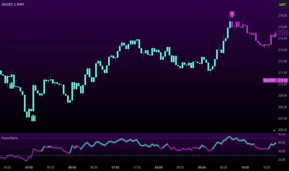
The Uptrick: FRAMA Matrix RSI is a momentum-based indicator that integrates the Relative Strength Index (RSI) with the Fractal Adaptive Moving Average (FRAMA). By applying FRAMA's adaptive smoothing to RSI—and further refining it with a Zero-Lag Moving Average (ZLMA)—this script creates a refined and reliable momentum oscillator. The indicator now includes enhanced divergence detection, potential reversal signals, customizable buy/sell signal options, an internal stats table, and a fully customizable bar coloring system for an enhanced visual trading experience.
Why Combine RSI with FRAMA
Traditional RSI is a well-known momentum indicator but has several limitations. It is highly sensitive to price fluctuations, often generating false signals in choppy or volatile markets. FRAMA, in contrast, adapts dynamically to price changes by adjusting its smoothing factor based on market conditions.
By integrating FRAMA into RSI calculations, this indicator reduces noise while preserving RSI's ability to track momentum, adapts to volatility by reducing lag in trending markets and smoothing out choppiness in ranging conditions, enhances trend-following capability for more reliable momentum shifts, and refines overbought and oversold signals by adjusting to the current market structure.
With the new enhancements, such as a manual alpha input, noise filtering, divergence detection, and multiple buy/sell signal options, the indicator offers even greater flexibility and precision for traders. This combination improves the standard RSI by making it more adaptive and responsive to market changes.
Originality
This indicator is unique because it applies FRAMA's adaptive smoothing technique to RSI, creating a dynamic momentum oscillator that adjusts to different market conditions. Many traditional RSI-based indicators either use fixed smoothing methods like exponential moving averages or employ basic RSI calculations without adjusting for volatility.
This script stands out by integrating several elements, including the fractal dimension-based smoothing of FRAMA to reduce noise while retaining responsiveness, the use of Zero-Lag Moving Average smoothing to enhance trend sensitivity and reduce lag, divergence detection to highlight mismatches between price action and RSI momentum, a noise filter and manual alpha option to prevent minor fluctuations from generating false signals, customizable buy/sell signal options that let traders choose between ZLMA-based or FRAMA RSI-based signals, an internal stats table displaying real-time FRAMA calculations such as fractal dimension and the adaptive alpha factor, and a fully customizable bar coloring system to visually distinguish bullish, bearish, and neutral conditions.
Features
Adaptive FRAMA RSI
The indicator applies FRAMA to RSI values, making the momentum oscillator adaptive to volatility while filtering out noise. Unlike a traditional RSI that reacts equally to all price movements, FRAMA RSI adjusts its smoothing factor based on market structure, making it more effective for identifying true momentum shifts.
Zero-Lag Moving Average (ZLMA)
A smoothing technique that minimizes lag while preserving the responsiveness of price movements. It is applied to the FRAMA RSI to further refine signals and ensure smoother trend detection.
Bullish and Bearish Threshold Crossovers
This system compares FRAMA RSI to a user-defined threshold (default is 50). When FRAMA RSI moves above the threshold, it indicates bullish momentum, while movement below signals bearish conditions. The enhanced noise filter ensures that only significant moves trigger signals.
Noise Filter and Manual Alpha
A new noise filter input prevents tiny fluctuations from triggering false signals. In addition, a manual alpha option allows traders to override the automatically computed smoothing factor with a custom value, providing extra control over the indicator’s sensitivity.
Divergence Detection
The indicator identifies divergence patterns by comparing FRAMA RSI pivots to price action. Bullish divergence occurs when price makes a lower low while FRAMA RSI makes a higher low, and bearish divergence occurs when price makes a higher high while FRAMA RSI makes a lower high. These signals can help traders anticipate potential reversals.
Reversal Signals
Labels appear on the chart when FRAMA RSI confirms classic RSI overbought (70) or oversold (30) conditions, providing visual cues for potential trend reversals.
Buy and Sell Signal Options
Traders can now choose between two signal-generation methods. ZLMA-based signals trigger when the ZLMA of FRAMA RSI crosses key overbought (70) or oversold (30) levels, while FRAMA RSI-based signals trigger when FRAMA RSI itself crosses these levels. This added flexibility allows users to tailor the indicator to their preferred trading style.
ZLMA:
FRAMA:
Customizable Alerts
Alerts notify traders when FRAMA RSI crosses key levels, divergence signals occur, reversal conditions are met, or buy/sell signals trigger. This ensures that important trading events are not missed.
Fully Customizable Bar Coloring System
Users can color bars based on different conditions, enhancing visual clarity. Bar coloring modes include: FRAMA RSI threshold (bars change color based on whether FRAMA RSI is above or below the threshold), ZLMA crossover (bars change when ZLMA crosses overbought or oversold levels), buy/sell signals (bars change when official signals trigger), divergence (bars highlight when bullish or bearish divergence is detected), and reversals (bars indicate when RSI reaches overbought or oversold conditions confirmed by FRAMA RSI). The system also remembers the last applied bar color, ensuring a smooth visual transition.
Input Parameters and Features
Core Inputs
RSI Length (default: 14) defines the period for RSI calculations.
FRAMA Lookback (default: 16) determines the length for the FRAMA smoothing function.
RSI Bull Threshold (default: 50) sets the level above which the market is considered bullish and below which it is bearish.
Noise Filter (default: 1.0) ensures that small fluctuations do not trigger false bullish or bearish signals.
Additional Features
Show Bull and Bear Alerts (default: true) enables notifications when FRAMA RSI crosses the threshold.
Enable Divergence Detection (default: false) highlights bullish and bearish divergences based on price and FRAMA RSI pivots.
Show Potential Reversal Signals (default: false) identifies overbought (70) and oversold (30) levels as possible trend reversal points.
Buy and Sell Signal Option (default: ZLMA) allows traders to choose between ZLMA-based signals or FRAMA RSI-based signals for trade entry.
ZLMA Enhancements
ZLMA Length (default: 14) determines the period for the Zero-Lag Moving Average applied to FRAMA RSI.
Visualization Options
Show Internal Stats Table (default: false) displays real-time FRAMA calculations, including fractal dimension and the adaptive alpha smoothing factor.
Show Threshold FRAMA Signals (default: false) plots buy and sell labels when FRAMA RSI crosses the threshold level.
How It Works
FRAMA Calculation
FRAMA dynamically adjusts smoothing based on the price fractal dimension. The alpha smoothing factor is derived from the fractal dimension or can be set manually to maintain responsiveness.
RSI with FRAMA Smoothing
RSI is calculated using the user-defined lookback period. FRAMA is then applied to the RSI to make it more adaptive to volatility. Optionally, ZLMA is applied to further refine the signals and reduce lag.
Bullish and Bearish Threshold Crosses
A bullish condition occurs when FRAMA RSI crosses above the threshold, while a bearish condition occurs when it falls below. The noise filter ensures that only significant trend shifts generate signals.
Buy and Sell Signal Options
Traders can choose between ZLMA crossovers or FRAMA RSI crossovers as the basis for buy and sell signals, offering flexibility in trade entry timing.
Divergence Detection
The indicator identifies divergences where price action and FRAMA RSI momentum do not align, potentially signaling upcoming reversals.
Reversal Signal Labels
When classic RSI overbought or oversold levels are confirmed by FRAMA RSI conditions, reversal labels are added on the chart to highlight potential exhaustion points.
Bar Coloring System
Bars are dynamically colored based on various conditions such as RSI thresholds, ZLMA crossovers, buy/sell signals, divergence, and reversals, allowing traders to quickly interpret market sentiment.
Alerts and Internal Stats
Customizable alerts notify traders of key events, and an optional internal stats table displays real-time calculations (fractal dimension, alpha value, and RSI values) to help users understand the underlying dynamics of the indicator.
Summary
The Uptrick: FRAMA Matrix RSI offers an enhanced approach to momentum analysis by combining RSI with adaptive FRAMA smoothing and additional layers of signal refinement. The indicator now includes adaptive RSI smoothing to reduce noise and improve responsiveness, Zero-Lag Moving Average filtering to minimize lag, divergence and reversal detection to identify potential turning points, customizable buy/sell signal options that let traders choose between different signal methodologies, a fully customizable bar coloring system to visually distinguish market conditions, and an internal stats table for real-time insight into FRAMA calculation parameters.
Whether used for trend confirmation, divergence detection, or momentum-based strategies, this indicator provides a powerful and adaptive approach to trading.
Disclaimer
This script is for informational and educational purposes only. Trading involves risk, and past performance does not guarantee future results. Always conduct proper research and consult with a financial advisor before making trading decisions.
Penunjuk Pine Script®