Daily Price LevelsTrack daily price action like a pro with instant visibility of key levels, percentages, and P&L values - all in one clean view."
Bullet points:
• Shows Daily Open, High, Low & Median levels
• Dynamic color-coding: green above open, red below
• Real-time price labels with:
Exact price levels
% distance between levels
Point values
Dollar values per contract
• Auto-repaints on timeframe changes
• 30min alerts for median crosses
Cari dalam skrip untuk "track"

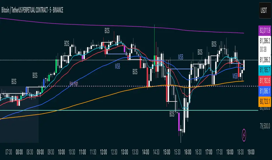
MSB BOS Market Structure [FTB]Track Market Structure Breaks (MSB) and Breaks of Structure (BOS) on your charts. This indicator does exactly that without clutter and with easy-to-spot.
🔑 Features:
MSB (Market Structure Break): Shows when price flips and breaks the previous high/low — possible start of a new trend.
BOS (Break of Structure): Highlights key structural breakouts in line with the existing trend.
✅ Pivot-Based Analysis (Body Focused)
Uses candle body-based pivot highs and lows to find clean market structure points (no wicks confusion here!).
Adjustable pivot strength — control how many candles you want on either side to define a swing.
✅ Clean Visual Markings
MSB and BOS lines with optional labels so you see exactly where breaks happen.
Customizable line style (Solid, Dashed, Dotted) to match your chart aesthetic.
Optional pivot markers to show minor swing highs/lows.
✅ Alerts Ready
Set alerts for any MSB or BOS, or filter to specific bullish/bearish breaks — never miss a key level again
💡 How to Use This Indicator:
Identify Trend Shifts: Use MSB to spot early trend reversals — when a previous structure breaks against the trend.
Catch Continuations: Watch for BOS to confirm trend continuation — great for riding the trend!
⚙️ Settings You Can Adjust:
Pivot Strength: How many candles to look back and forward for swing points (default: 3).
Show Pivots: Optional — highlight swing highs and lows for extra clarity.
Federal Funds Rate Projections [tedtalksmacro]Track the Federal Funds Rate projections for each month via the Fed Funds Rate Futures Contracts CBOT:ZQ1!
This will be updated monthly to ensure that the current and relevant contracts are implemented.
Traders can use this to speculate on whether the Federal Reserve is likely to raise, cut or do nothing to their key interest rate at the next meeting.

FANG INDICATORTrack the strength of any group of stocks that are driving markets. This defaults to FANG. In the settings, replace the symbols to better fit the environment such as replacing NFLX with AAPL.

Multi Timeframe Rolling Bitmex Liquidation LevelsTrack Bitmex liquidations levels in real-time with a rolling VWMA or VWAP basis.
Allows the input of a different time frame if you wish.

200/100 vs 190/80 EMA [jarederaj]Track the 200/100 EMA cross Vs the 180/90 EMA cross. Also, see the dates when these periods start on the chart.
Consecutive Highs/LowsTrack consecutive new highs/lows outside the Donchian range. Fans of the oldschool Turtle Strategy should enjoy the visualization.
Same logic as my "Walking the Bands" script, just with Donchian breaks instead of Bollinger tags.


Altcoin PortfolioTrack your altcoin portfolio balance in Fiat currency.
Make sure to open the data window to the right of your charts, it makes everything alot easier to read at a glance.
To learn more about customizing this script to fit your portfolio, watch the video here: youtu.be
To get more cool scripts and up-to-date information about Autoview, join us in slack slack.with.pink
As per the usual, we hope this script helps with your trading venture.
Good luck, and happy trading.

QQQ/ES Overlay on NQQQQ/ES Overlay on NQ
This indicator overlays QQQ or ES price levels onto your NQ chart, dynamically mapping reference levels from your chosen symbol to equivalent NQ prices. Perfect for tracking correlations between Nasdaq futures and related instruments.
Key Features
Dual Symbol Support - Toggle between QQQ and ES with a dropdown. Each symbol uses optimized defaults: QQQ shows every 1 point, ES shows every 5 points.
Pre-Market Ready - Extended session support starting at 4:00 AM ET captures pre-market movement. By 9:00 AM, levels accurately reflect overnight action.
Smart Level Mapping - Calculates real-time ratio between NQ and your overlay symbol, then maps round price levels (like QQQ 614 or ES 5985) to equivalent NQ prices.
Anti-Jitter Technology - Stability threshold prevents lines from shaking on minor movements while maintaining accuracy.
How It Works
The indicator fetches live prices from both QQQ and ES, calculates the dynamic ratio to NQ, and displays mapped reference levels. For example, if NQ trades at 21,500 and QQQ at 614, the ratio is approximately 35.016. This means QQQ 615 maps to roughly 21,535 on your NQ chart.
Customization
Choose overlay source (QQQ or ES)
Adjust level increments independently for each symbol
Set number of levels above/below price
Customize line style, width, and color
Control label appearance and position
Fine-tune update sensitivity
Use Cases
Track market correlations in real-time, identify divergences between instruments, trade off psychological round numbers from correlated markets, monitor pre-market relationships, and maintain consistent reference levels across timeframes.
Settings
Default configuration shows 20 levels above and below current price with white lines at 40% opacity. QQQ uses 1-point increments, ES uses 5-point increments. Labels appear 8 bars to the right with dashed lines. Minimum 0.5-point move required to update positions.
Technical Notes
Designed specifically for NQ charts. Uses extended session data (4:00 AM - 8:00 PM ET) for live calculations. Outside trading hours, maintains ratio from previous close. Real-time updates depend on active data feed for all symbols.

Customizable Macro If you’re strategy relies on time then this indicator allows you to customize specific time windows to show so you no longer have to manually keep track of the time.
Freebird Flow MomentumHello, TradingView Comm;
This is a simple "3-Speed" Momentum Flow Tracker.
It is designed to give traders early signal to shifts of Buy/Sell Momentum-over-Time at all timeframes for the purpose of targeting accurate entry/exit on the micro, while still maintaining full integrity and viability while macro timeframe charting.
This indicator adds in a separate pane by default.
It can, and was designed to however, be combined with your Price Chart. IF you choose to do so:
- Fixed Center Alignment + Price Pan "Bonus": '0.00'-line acts as a "Net" indicator. When Zero line above median of pane, Sellers are the "Net" winners of the candles in view, and vice versa. The distance from center indicates Magnitude of Net Imbalance.
Recommended Opacity Settings:
- Histogram: 20-25%
- Cloud: 33-40%
USD Liquidity Regime for BTC Perps (Dual) V1USD Liquidity Regime for BTC Perps (Dual)
This intents to be a BTC Perps USD Liquidity Regime macro indicator.
As it names states it is designed for BTCUSDT perpetual futures traders.
It attempts to tracks USD strength (DXY, UUP, yields, VIX composite) as liquidity proxy:
Lower index = weak USD = Risk-On (green background/histogram = long tailwind for BTC).
Higher = strong USD = Risk-Off (red = caution longs, shorts favor).
How to use:
Green background/histogram: Favor longs — rallies likely, dips bought.
Red: Caution longs — corrections hurt, short bias possible.
Blue line (index) vs red SMA: Crosses signal regime shifts.
Histogram strength: Bigger bars = stronger bias.
This is not intended as financial advise or trigger signal tool.
This is a work in progress
Its value is limited, if you do not understand any or some of the words above please do not use this indicator. If you did, then you understand you are not supposed to use this alone to make decisions.
Feel free to ask any questions, this is a work in progress.
Feel free to suggest improvements.
Educational macro context tool — not signals/advice.
Ok for avoiding going against the USD trend dominance by following liquidity.
By @frank_vergaram

PMax & MOST SynergyIntroduction
This script brings together two of the most powerful trend-following and volatility-based trailing stop-loss indicators in the technical analysis world: Profit Maximizer (PMax) and Moving Stop Loss (MOST). By merging these two tools into a single, optimized script, this indicator aims to reduce chart clutter while providing a comprehensive trend-tracking solution. Both indicators are integrated with their original logic and default parameters, now fully compatible with the latest Pine Script v5 standards.
Development & Technical Logic
The indicator is designed for versatility, allowing traders to monitor dual layers of protection and trend confirmation.
PMax Integration: It utilizes the volatility-adjusted trailing stop-loss logic combined with a variety of selectable Moving Average types (SMA, EMA, VAR, etc.). In this version, the default PMax settings are pre-configured to utilize the Variable Moving Average (VAR) to ensure smoother trend detection with reduced lag.
MOST Integration: The script includes the Moving Stop Loss (MOST) logic, which provides a dynamic exit strategy based on percentage-based trailing stops.
Visual Enhancements: The PMax line has been visually updated to a distinct Blue color for better clarity, and all secondary signals (Support/Resistance lines and highlights) are set to be optional to keep the interface clean and professional.
Conclusion
This combined version is an ideal tool for trend followers who want to benefit from multiple confirmation layers. Whether you are looking for long-term trend stability with PMax or tactical exit/entry signals with MOST, this script provides the flexibility to adjust both independently. It eliminates the need for multiple indicator slots and offers a unified dashboard for trend analysis across various timeframes and assets.
Acknowledgements
I would like to express my sincere gratitude to the original developers who designed these essential tools:
Kivanc Ozbilgic (@KivancOzbilgic): Thank you for your immense contribution to the trading community and for developing the Profit Maximizer (PMax). Your work continues to be a cornerstone for many traders worldwide.
Ceyhun (@ceyhun): A special thanks for designing the Moving Stop Loss (MOST) indicator. Your innovative approach to trailing stops has significantly improved how we manage risk in the markets.

[Algo/Fract] Quant+Built for traders ready to Level Up.
Combine algorithmic strength tracking with fractal structure to deliver quant-style clarity on a live chart.
You trade with intuition. Quant trades with Data.
Together, you read the Unseen.
Quant+ is the second component of the AlgoFract Quant Suite.
Features included are:
Quant Cycles & Ghost Cycle (QC)
Custom Volume Spread (VS)
Volume Flow (VF)
Gain Access at: www.algofract.com
or by visiting our Whop Marketplace: whop.com

Enigma UnlockedENIGMA Indicator: A Comprehensive Market Bias & Success Tracker
The ENIGMA Indicator is a powerful tool designed for traders who aim to identify market bias, track price movements, and evaluate trade performance using multiple timeframes. It combines multiple indicators and advanced logic to provide real-time insights into market trends, helping traders make more informed decisions.
Key Features
1. Multi-Timeframe Bias Calculation:
The ENIGMA Indicator tracks the market bias across multiple timeframes—Daily (D), 4-Hour (H4), 1-Hour (H1), 30-Minute (30M), 15-Minute (15M), 5-Minute (5M), and 1-Minute (1M).
How the Bias is Created:
The Bias is a key feature of the ENIGMA Indicator and is determined by comparing the current price with previous price levels for each timeframe.
- Bullish Bias (1): The market is considered **bullish** if the **current closing price** is higher than the **previous timeframe’s high**. This suggests that the market is trending upwards, and buyers are in control.
- Bearish Bias (-1): The market is considered **bearish** if the **current closing price** is lower than the **previous timeframe’s low**. This suggests that the market is trending downwards, and sellers are in control.
- Neutral Bias (0): The market is considered **neutral** if the price is between the **previous high** and **previous low**, indicating indecision or a range-bound market.
This bias calculation is performed independently for each timeframe. The **Bias** for each timeframe is then displayed in the **Bias Table** on your chart, providing a clear view of market direction across multiple timeframes.
2. **Customizable Table Display:**
- The indicator provides a table that displays the bias for each selected timeframe, clearly marking whether the market is **Bullish**, **Bearish**, or **Neutral**.
- Users can choose where to place the table on the chart: top-left, top-right, bottom-left, bottom-right, or center positions, allowing for easy and personalized chart management.
3. **Win/Loss Tracker:**
- The table also tracks the **success rate** of **buy** and **sell** trades based on price retests of key bias levels.
- For each period (Day, Week, Month), it tracks how often the price has moved in the direction of the initial bias, counting **Buy Wins**, **Sell Wins**, **Buy Losses**, and **Sell Losses**.
- This helps traders assess the effectiveness of the market bias over time and adjust their strategies accordingly.
#### **How the Success Calculation Determines the Success Rate:**
The **Success Calculation** is designed to track how often the price follows the direction of the market bias. It does this by evaluating how the price retests key levels associated with the identified market bias:
1. **Buy Success Calculation**:
- The success of a **Buy Trade** is determined when the price breaks above the **previous high** after a **bullish bias** has been identified.
- If the price continues to move higher (i.e., makes a new high) after breaking the previous high, the **buy trade is considered successful**.
- The indicator tracks how many times this condition is met and counts it as a **Buy Win**.
2. **Sell Success Calculation**:
- The success of a **Sell Trade** is determined when the price breaks below the **previous low** after a **bearish bias** has been identified.
- If the price continues to move lower (i.e., makes a new low) after breaking the previous low, the **sell trade is considered successful**.
- The indicator tracks how many times this condition is met and counts it as a **Sell Win**.
3. **Failure Calculations**:
- If the price does not move as expected (i.e., it does not continue in the direction of the identified bias), the trade is considered a **loss** and is tracked as **Buy Loss** or **Sell Loss**, depending on whether it was a bullish or bearish trade.
The ENIGMA Indicator keeps a running tally of **Buy Wins**, **Sell Wins**, **Buy Losses**, and **Sell Losses** over a set period (which can be customized to Days, Weeks, or Months). These statistics are updated dynamically in the **Bias Table**, allowing you to track your success rate in real-time and gain insights into the effectiveness of the market bias.
#### **Customizable Period Tracking:**
- The ENIGMA Indicator allows you to set custom tracking periods (e.g., 30 days, 2 weeks, etc.). The performance metrics reset after each tracking period, helping you monitor your success in different market conditions.
5. **Interactive Settings:**
- **Lookback Period**: Define how many bars the indicator should consider for bias calculations.
- **Success Tracking**: Set the number of candles to track for calculating the win/loss performance.
- **Time Threshold**: Set a time threshold to help define the period during which price retests are considered valid.
- **Info Tooltip**: You can enable the information tool in the settings to view detailed explanations of how wins and losses are calculated, ensuring you understand how the indicator works and how the results are derived.
#### **How to Use the ENIGMA Indicator:**
1. **Install the Indicator**:
- Add the ENIGMA Indicator to your chart. It will automatically calculate and display the bias for multiple timeframes.
2. **Interpret the Bias Table**:
- The bias table will show whether the market is **Bullish**, **Bearish**, or **Neutral** across different timeframes.
- Look for alignment between the timeframes—when multiple timeframes show the same bias, it may indicate a stronger trend.
3. **Use the Win/Loss Tracker**:
- Track how well your trades align with the bias using the **Win/Loss Tracker**. This helps you refine your strategy by understanding which timeframes and biases lead to higher success rates.
- For example, if you see a high number of **Buy Wins** and a low number of **Sell Wins**, you may decide to focus more on buying during bullish trends and avoid selling during bearish retracements.
4. **Track Your Period Performance**:
- The indicator will automatically track your performance over the set period (Days, Weeks, Months). Use this data to adjust your approach and evaluate the effectiveness of your trading strategy.
5. **Position the Table**:
- Customize the placement of the table on your chart based on your preferences. You can choose from options like **Top Left**, **Top Right**, **Bottom Left**, **Bottom Right**, or **Center** to keep the chart uncluttered.
6. **Adjust Settings**:
- Modify the indicator settings according to your trading style. You can adjust the **Lookback Period**, **Number of Candles to Track**, and **Time Threshold** to match the pace of your trading.
7. **Use the Info Tooltip**:
- Enable the **Info Tool** in the settings to understand how the Buy/Sell Wins and Losses are calculated. The tooltip provides a breakdown of how the indicator tracks price movements and calculates the success rate.
**Conclusion:**
The **ENIGMA Indicator** is designed to help traders make informed decisions by providing a clear view of the market bias and performance data. With the ability to track bias across multiple timeframes and evaluate your trading success, it can be a powerful tool for refining your trading strategies.
Whether you're looking to focus on a single timeframe or analyze multiple timeframes for a stronger bias, the ENIGMA Indicator adapts to your needs, providing both real-time market insights and performance feedback.
Major Crypto Relative Strength Portfolio System Majors RSPS - Relative Strength Portfolio System for Major Cryptocurrencies
Overview
Majors RSPS (Relative Strength Portfolio System) is an advanced portfolio allocation indicator that combines relative strength analysis, trend consensus, and macro risk factors to dynamically allocate capital across major cryptocurrency assets. The system leverages the NormalizedIndicators Library to evaluate both absolute trends and relative performance, creating an adaptive portfolio that automatically adjusts exposure based on market conditions.
This indicator is designed for portfolio managers, asset allocators, and systematic traders who want a data-driven approach to cryptocurrency portfolio construction with automatic rebalancing signals.
🎯 Core Concept
What is RSPS?
RSPS (Relative Strength Portfolio System) evaluates each asset on two key dimensions:
Relative Strength: How is the asset performing compared to other major cryptocurrencies?
Absolute Trend: Is the asset itself in a bullish trend?
Assets that show both strong relative performance AND positive absolute trends receive higher allocations. Weak performers are automatically filtered out, with capital reallocated to cash or stronger assets.
Dual-Layer Architecture
Layer 1: Majors Portfolio (Orange Zone)
Evaluates 14 major cryptocurrency assets
Calculates relative strength against all other majors
Applies trend filters to ensure absolute momentum
Dynamically allocates capital based on comparative strength
Layer 2: Cash/Risk Position (Navy Zone)
Evaluates macro risk factors and market conditions
Determines optimal cash allocation
Acts as a risk-off mechanism during adverse conditions
Provides downside protection through dynamic cash holdings
📊 Tracked Assets
Major Cryptocurrencies (14 Assets)
BTC - Bitcoin (Benchmark L1)
ETH - Ethereum (Smart Contract L1)
SOL - Solana (High-Performance L1)
SUI - Sui (Move-Based L1)
TRX - Tron (Payment-Focused L1)
BNB - Binance Coin (Exchange L1)
XRP - Ripple (Payment Network)
FTM - Fantom (DeFi L1)
CELO - Celo (Mobile-First L1)
TAO - Bittensor (AI Network)
HYPE - Hyperliquid (DeFi Exchange)
HBAR - Hedera (Enterprise L1)
ADA - Cardano (Research-Driven L1)
THETA - Theta (Video Network)
🔧 How It Works
Step 1: Relative Strength Calculation
For each asset, the system calculates relative strength by:
RSPS Score = Average of:
- Asset/BTC trend consensus
- Asset/ETH trend consensus
- Asset/SOL trend consensus
- Asset/SUI trend consensus
- ... (all 14 pairs)
- Asset's absolute trend consensus
Key Logic:
Each pair is evaluated using the eth_4d_cal() calibration from NormalizedIndicators
If an asset's absolute trend is extremely weak (≤ 0.1), it receives a penalty score (-0.5)
Otherwise, it gets the average of all its relative strength comparisons
Step 2: Trend Filtering
Assets must pass a trend filter to receive allocation:
Trend Score = Average of:
- Asset/BTC trend (filtered for positivity)
- Asset/ETH trend (filtered for positivity)
- Asset's absolute trend (filtered for positivity)
Only positive values contribute to the trend score, ensuring bearish assets don't receive allocation.
Step 3: Portfolio Allocation
Capital is allocated proportionally based on filtered RSPS scores:
Asset Allocation % = (Asset's Filtered RSPS Score / Sum of All Filtered Scores) × Main Portfolio %
Example:
SOL filtered score: 0.6
BTC filtered score: 0.4
All others: 0
Total: 1.0
SOL receives: (0.6 / 1.0) × Main% = 60% of main portfolio
BTC receives: (0.4 / 1.0) × Main% = 40% of main portfolio
Step 4: Cash/Risk Allocation
The system evaluates macro conditions across 6 factors:
Inverse Major Crypto Trends (40% weight)
When BTC, ETH, SOL, SUI, DOGE, etc. trend down → Cash allocation increases
Evaluates total market cap trends (TOTAL, TOTAL2, OTHERS)
Stablecoin Dominance (10% weight)
USDC dominance vs. major crypto dominances
Higher stablecoin dominance → Higher cash allocation
MVRV Ratios (10% weight)
BTC and ETH Market Value to Realized Value
High MVRV (overvaluation) → Higher cash allocation
BTC/ETH Ratio (15% weight)
Relative performance between two market leaders
Indicates market phase (BTC dominance vs. alt season)
Active Address Ratios (5% weight)
USDC active addresses vs. BTC/ETH active addresses
Network activity comparison
Macro Indicators (15% weight)
Global currency circulation (USD, EUR, CNY, JPY)
Treasury yield curve (10Y-2Y)
High yield spreads
Central bank balance sheets and money supply
Cash Allocation Formula:
Cash % = (Sum of Risk Factors × 0.5) / (Risk Factors + Majors TPI)
When risk factors are elevated, cash allocation increases, reducing exposure to volatile assets.
📈 Visual Components
Orange Zone (Majors Portfolio)
Fill: Light orange area showing aggregate portfolio strength
Line: Average trend power index (TPI) of allocated assets
Baseline: 0 level (neutral)
Interpretation:
Above 0: Bullish allocation environment
Rising: Strengthening portfolio momentum
Falling: Weakening portfolio momentum
Below 0: No allocation (100% cash)
Navy Zone (Cash Position)
Fill: Navy blue area showing cash allocation strength
Line: Risk-adjusted cash allocation signal
Baseline: 0 level
Interpretation:
Higher navy zone: Elevated risk-off signal → More cash
Lower navy zone: Risk-on environment → Less cash
Zero: No cash allocation (100% invested)
Performance Line (Orange/Blue)
Orange: Main portfolio allocation dominant (risk-on mode)
Blue: Cash allocation dominant (risk-off mode)
Tracks: Cumulative portfolio returns with dynamic rebalancing
Allocation Table (Bottom Left)
Shows real-time portfolio composition:
ColumnDescriptionAssetCryptocurrency nameRSPS ValuePercentage allocation (of main portfolio)CashDollar amount (if enabled)
Color Coding:
Orange: Active allocation
Gray: Weak signal (borderline)
Blue: Cash position
Missing: No allocation (filtered out)
⚙️ Settings & Configuration
Required Setup
Chart Symbol
MUST USE: INDEX:BTCUSD or similar major crypto index
Recommended Timeframe: 1D (Daily) or 4D (4-Day)
Why: System needs price data for all 14 majors, BTC provides stable reference
Hide Chart Candles
For clean visualization:
Right-click on chart
Select "Hide Symbol" or set candle opacity to 0
This allows the indicator fills and table to be clearly visible
User Inputs
plot_table (Default: true)
Enable/disable the allocation table
Set to false if you only want the visual zones
use_cash (Default: false)
Enable portfolio dollar value calculations
Shows actual dollar allocations per asset
cash (Default: 100)
Total portfolio size in dollars/currency units
Used when use_cash is enabled
Example: Set to 10000 for a $10,000 portfolio
💡 Interpretation Guide
Entry Signals
Strong Allocation Signal:
✓ Orange zone elevated (> 0.3)
✓ Navy zone low (< 0.2)
✓ Performance line orange
✓ Multiple assets in allocation table
→ Action: Deploy capital to allocated assets per table percentages
Risk-Off Signal:
✓ Orange zone near zero
✓ Navy zone elevated (> 0.4)
✓ Performance line blue
✓ Few or no assets in table (high cash %)
→ Action: Reduce exposure, increase cash holdings
Rebalancing Triggers
Monitor the allocation table for changes:
New assets appearing: Add to portfolio
Assets disappearing: Remove from portfolio
Percentage changes: Rebalance existing positions
Cash % changes: Adjust overall exposure
Market Regime Detection
Risk-On (Bull Market):
Orange zone high and rising
Navy zone minimal
Many assets allocated (8-12)
High individual allocations (15-30% each)
Risk-Off (Bear Market):
Orange zone near zero or negative
Navy zone elevated
Few assets allocated (0-3)
Cash allocation dominant (70-100%)
Transition Phase:
Both zones moderate
Medium number of assets (4-7)
Balanced cash/asset allocation (40-60%)
🎯 Trading Strategies
Strategy 1: Pure RSPS Following
1. Check allocation table daily
2. Rebalance portfolio to match percentages
3. Follow cash allocation strictly
4. Review weekly, act on significant changes (>5%)
Best For: Systematic portfolio managers, passive allocators
Strategy 2: Threshold-Based
Entry Rules:
- Orange zone > 0.4 AND Navy zone < 0.3
- At least 5 assets in allocation table
- Total non-cash allocation > 60%
Exit Rules:
- Orange zone < 0.1 OR Navy zone > 0.5
- Fewer than 3 assets allocated
- Cash allocation > 70%
Best For: Active traders wanting clear rules
Strategy 3: Relative Strength Overlay
1. Use RSPS for broad allocation framework
2. Within allocated assets, overweight top 3 performers
3. Scale position sizes by RSPS score
4. Use individual asset charts for entry/exit timing
Best For: Discretionary traders with portfolio focus
Strategy 4: Risk-Adjusted Position Sizing
For each allocated asset:
Position Size = Base Position × (Asset's RSPS Score / Max RSPS Score) × (1 - Cash Allocation)
Example:
- $10,000 portfolio
- SOL RSPS: 0.6 (highest)
- BTC RSPS: 0.4
- Cash allocation: 30%
SOL Size = $10,000 × (0.6/0.6) × (1-0.30) = $7,000
BTC Size = $10,000 × (0.4/0.6) × (1-0.30) = $4,667
Cash = $10,000 × 0.30 = $3,000
Best For: Risk-conscious allocators
📊 Advanced Usage
Multi-Timeframe Confirmation
Use on multiple timeframes for robust signals:
1D Chart: Tactical allocation (daily rebalancing)
4D Chart: Strategic allocation (weekly review)
Strong Confirmation:
- Both timeframes show same top 3 assets
- Both show similar cash allocation levels
- Orange zones aligned on both
Weak/Conflicting:
- Different top performers
- Diverging cash allocations
→ Wait for alignment or use shorter timeframe
Sector Rotation Analysis
Group assets by type and watch rotation:
L1 Dominance: BTC, ETH, SOL, SUI, ADA high → Layer 1 season
Alt L1s: TRX, FTM, CELO rising → Alternative platform season
Specialized: TAO, THETA, HYPE strong → Niche narrative season
Payment/Stable: XRP, BNB allocation → Risk reduction phase
Divergence Trading
Bullish Divergence:
Navy zone declining (less risk-off)
Orange zone flat or slightly rising
Few assets still allocated but strengthening
→ Early accumulation signal
Bearish Divergence:
Orange zone declining
Navy zone rising
Asset count decreasing in table
→ Distribution/exit signal
Performance Tracking
The performance line (overlay) shows cumulative strategy returns:
Compare to BTC/ETH: Is RSPS outperforming?
Drawdown analysis: How deep are pullbacks?
Correlation: Does it track market or provide diversification?
🔬 Technical Details
Data Sources
Price Data:
COINEX: Primary exchange for alt data
CRYPTO: Alternative price feeds
INDEX: Aggregated index prices (recommended for BTC)
Macro Data:
Dominance metrics (SUI.D, BTC.D, etc.)
MVRV ratios (on-chain valuation)
Active addresses (network activity)
Global money supply and macro indicators
Calculation Methodology
RSPS Scoring:
For each asset, calculate 14 relative trends (vs. all others)
Calculate asset's absolute trend
Average all 15 values
Apply penalty filter for extremely weak trends (≤ 0.1)
Trend Consensus:
Uses eth_4d_cal() from NormalizedIndicators library
Combines 8 normalized indicators per measurement
Returns value from -1 (bearish) to +1 (bullish)
Performance Calculation:
Daily Return = Σ(Asset ROC × Asset Allocation)
Cumulative Performance = Previous Perf × (1 + Daily Return / 100)
Assumes perfect rebalancing and no slippage (theoretical performance).
Filtering Logic
filter() function:
pinescriptfilter(input) => input >= 0 ? input : 0
This zero-floor filter ensures:
Only positive trend values contribute to allocation
Bearish assets receive 0 weight
No short positions or inverse allocations
Anti-Manipulation Safeguards
Null Handling:
All values wrapped in nz() to handle missing data
Prevents calculation errors from data gaps
Normalization:
Allocations always sum to 100%
Prevents over/under-allocation
Conditional Logic:
Assets need positive values on multiple metrics
Single metric cannot drive allocation alone
⚠️ Important Considerations
Required Timeframes
1D (Daily): Recommended for most users
4D (4-Day): More stable, fewer rebalances
Other timeframes: Use at your own discretion, may require recalibration
Data Requirements
Needs INDEX:BTCUSD or equivalent major crypto symbol
All 14 tracked assets must have available data
Macro indicators require specific TradingView data feeds
Rebalancing Frequency
System provides daily allocation updates
Practical rebalancing: Weekly or on significant changes (>10%)
Consider transaction costs and tax implications
Performance Notes
Theoretical returns: No slippage, fees, or execution delays
Backtest carefully: Validate on your specific market conditions
Past performance: Does not guarantee future results
Risk Warnings
⚠️ High Concentration Risk: May allocate heavily to 1-3 assets
⚠️ Volatility: Crypto markets are inherently volatile
⚠️ Liquidity: Some allocated assets may have lower liquidity
⚠️ Correlation: All assets correlated to BTC/ETH to some degree
⚠️ System Risk: Relies on continued availability of data feeds
Not Financial Advice
This indicator is a tool for analysis and research. It does not constitute:
Investment advice
Portfolio management services
Trading recommendations
Guaranteed returns
Always perform your own due diligence and risk assessment.
🎓 Use Cases
For Portfolio Managers
Systematic allocation framework
Objective rebalancing signals
Risk-adjusted exposure management
Performance tracking vs. benchmarks
For Active Traders
Identify strongest assets to focus trading on
Gauge overall market regime (risk-on/off)
Time entry/exit for portfolio shifts
Complement technical analysis with allocation data
For Institutional Allocators
Quantitative portfolio construction
Multi-asset exposure optimization
Drawdown management through cash allocation
Compliance-friendly systematic approach
For Researchers
Study relative strength dynamics in crypto markets
Analyze correlation between majors
Test macro factor impact on crypto allocations
Develop derived strategies and signals
🔧 Setup Checklist
✅ Chart Configuration
Set chart to INDEX:BTCUSD
Set timeframe to 1D or 4D
Hide chart candles for clean visualization
Add indicator from library
✅ Indicator Settings
Enable plot_table (see allocation table)
Set use_cash if tracking dollar amounts
Input your portfolio size in cash parameter
✅ Monitoring Setup
Bookmark chart for daily review
Set alerts for major allocation changes (optional)
Create spreadsheet to track allocations (optional)
Establish rebalancing schedule (weekly recommended)
✅ Validation
Verify all 14 assets appear in table (when allocated)
Check that percentages sum to ~100%
Confirm performance line is tracking
Test cash allocation calculation if enabled
📋 Quick Reference
Signal Interpretation
ConditionOrange ZoneNavy ZoneActionStrong BullHigh (>0.4)Low (<0.2)Full allocationModerate BullMid (0.2-0.4)Low-MidStandard allocationNeutralLow (0.1-0.2)Mid (0.3-0.4)Balanced allocationModerate BearVery Low (<0.1)Mid-HighReduce exposureStrong BearZero/NegativeHigh (>0.5)High cash/exit
Rebalancing Thresholds
Change TypeThresholdActionIndividual asset±5%Consider rebalanceIndividual asset±10%Strongly rebalanceCash allocation±10%Adjust exposureAsset entry/exitAnyAdd/remove position
Color Legend
Orange: Main portfolio strength/allocation
Navy: Cash/risk-off allocation
Blue text: Cash position in table
Orange text: Active asset allocation
Gray text: Weak/borderline allocation
White: Headers and labels
🚀 Getting Started
Beginner Path
Add indicator to INDEX:BTCUSD daily chart
Hide candles for clarity
Enable plot_table to see allocations
Check table daily, note top 3-5 assets
Start with small allocation, observe behavior
Gradually increase allocation as you gain confidence
Intermediate Path
Set up on both 1D and 4D charts
Enable use_cash with your portfolio size
Create tracking spreadsheet
Implement weekly rebalancing schedule
Monitor divergences between timeframes
Compare performance to buy-and-hold BTC
Advanced Path
Modify code to add/remove tracked assets
Adjust relative strength calculation methodology
Customize cash allocation factors and weights
Integrate with portfolio management platform
Develop algorithmic rebalancing system
Create alerts for specific allocation conditions
📖 Additional Resources
Related Indicators
NormalizedIndicators Library: Core calculation engine
Individual asset trend indicators for deeper analysis
Macro indicator dashboards for cash allocation factors
Complementary Analysis
On-chain metrics (MVRV, active addresses, etc.)
Order book liquidity for execution planning
Correlation matrices for diversification analysis
Volatility indicators for position sizing
Learning Materials
Study relative strength portfolio theory
Research tactical asset allocation strategies
Understand crypto market cycles and phases
Learn about risk management in volatile assets
🎯 Key Takeaways
✅ Systematic allocation across 14 major cryptocurrencies
✅ Dual-layer approach: Asset selection + Cash management
✅ Relative strength focused: Invests in comparatively strong assets
✅ Trend filtering: Only allocates to assets in positive trends
✅ Dynamic rebalancing: Automatically adjusts to market conditions
✅ Risk-managed: Increases cash during adverse conditions
✅ Transparent methodology: Clear calculation logic
✅ Practical visualization: Easy-to-read table and zones
✅ Performance tracking: See cumulative strategy returns
✅ Highly customizable: Adjust assets, weights, and factors
📋 License
This code is subject to the Mozilla Public License 2.0 at mozilla.org
Majors RSPS transforms complex multi-asset portfolio management into a systematic, data-driven process. By combining relative strength analysis with trend consensus and macro risk factors, it provides traders and portfolio managers with a robust framework for navigating cryptocurrency markets with discipline and objectivity.WiederholenClaude kann Fehler machen. Bitte überprüfen Sie die Antworten. Sonnet 4.5

Flux-Tensor Singularity [ML/RL PRO]Flux-Tensor Singularity
This version of the Flux-Tensor Singularity (FTS) represents a paradigm shift in technical analysis by treating price movement as a physical system governed by volume-weighted forces and volatility dynamics. Unlike traditional indicators that measure price change or momentum in isolation, FTS quantifies the complete energetic state of the market by fusing three fundamental dimensions: price displacement (delta_P), volume intensity (V), and local-to-global volatility ratio (gamma).
The Physics-Inspired Foundation:
The tensor calculation draws inspiration from general relativity and fluid dynamics, where massive objects (large volume) create curvature in spacetime (price action). The core formula:
Raw Singularity = (ΔPrice × ln(Volume)) × γ²
Where:
• ΔPrice = close - close (directional force)
• ln(Volume) = logarithmic volume compression (prevents extreme outliers)
• γ (Gamma) = (ATR_local / ATR_global)² (volatility expansion coefficient)
This raw value is then normalized to 0-100 range using the lookback period's extremes, creating a bounded oscillator that identifies critical density points—"singularities" where normal market behavior breaks down and explosive moves become probable.
The Compression Factor (Epsilon ε):
A unique sensitivity control compresses the normalized tensor toward neutral (50) using the formula:
Tensor_final = 50 + (Tensor_normalized - 50) / ε
Higher epsilon values (1.5-3.0) make threshold breaches rare and significant, while lower values (0.3-0.7) increase signal frequency. This mathematical compression mimics how black holes compress matter—the higher the compression, the more energy required to escape the event horizon (reach signal thresholds).
Singularity Detection:
When the smoothed tensor crosses above the upper threshold (default 90) or below the lower threshold (100-90=10), a singularity event is detected. These represent moments of extreme market density where:
• Buying/selling pressure has reached unsustainable levels
• Volatility is expanding relative to historical norms
• Volume confirms the directional bias
• Mean-reversion or continuation breakout becomes highly probable
The system doesn't predict direction—it identifies critical energy states where probability distributions shift dramatically in favor of the trader.
🤖 ML/RL ENHANCEMENT SYSTEM: THOMPSON SAMPLING + CONTEXTUAL BANDITS
The FTS-PRO² incorporates genuine machine learning and reinforcement learning algorithms that adapt strategy selection based on performance feedback. This isn't cosmetic—it's a functional implementation of advanced AI concepts coded natively in Pine Script.
Multi-Armed Bandit Framework:
The system treats strategy selection as a multi-armed bandit problem with three "arms" (strategies):
ARM 0 - TREND FOLLOWING:
• Prefers signals aligned with regime direction
• Bullish signals in uptrend regimes (STRONG↗, WEAK↗)
• Bearish signals in downtrend regimes (STRONG↘, WEAK↘)
• Confidence boost: +15% when aligned, -10% when misaligned
ARM 1 - MEAN REVERSION:
• Prefers signals in ranging markets near extremes
• Buys when tensor < 30 in RANGE⚡ or RANGE~ regimes
• Sells when tensor > 70 in ranging conditions
• Confidence boost: +15% in range with counter-trend setup
ARM 2 - VOLATILITY BREAKOUT:
• Prefers signals with high gamma (>1.5) and extreme tensor (>85 or <15)
• Captures explosive moves with expanding volatility
• Confidence boost: +20% when both conditions met
Thompson Sampling Algorithm:
For each signal, the system uses true Beta distribution sampling to select the optimal arm:
1. Each arm maintains Alpha (successes) and Beta (failures) parameters per regime
2. Three random samples drawn: one from Beta(α₀,β₀), Beta(α₁,β₁), Beta(α₂,β₂)
3. Highest sample wins and that arm's strategy applies
4. After trade outcome:
- Win → Alpha += 1.0, reward += 1.0
- Loss → Beta += 1.0, reward -= 0.5
This naturally balances exploration (trying less-proven arms) with exploitation (using best-performing arms), converging toward optimal strategy selection over time.
Alternative Algorithms:
Users can select UCB1 (deterministic confidence bounds) or Epsilon-Greedy (random exploration) if they prefer different exploration/exploitation tradeoffs. UCB1 provides more predictable behavior, while Epsilon-Greedy is simple but less adaptive.
Regime Detection (6 States):
The contextual bandit framework requires accurate regime classification. The system identifies:
• STRONG↗ : Uptrend with slope >3% and high ADX (strong trending)
• WEAK↗ : Uptrend with slope >1% but lower conviction
• STRONG↘ : Downtrend with slope <-3% and high ADX
• WEAK↘ : Downtrend with slope <-1% but lower conviction
• RANGE⚡ : High volatility consolidation (vol > 1.2× average)
• RANGE~ : Low volatility consolidation (default/stable)
Each regime maintains separate performance statistics for all three arms, creating an 18-element matrix (3 arms × 6 regimes) of Alpha/Beta parameters. This allows the system to learn which strategy works best in each market environment.
🧠 DUAL MEMORY ARCHITECTURE
The indicator implements two complementary memory systems that work together to recognize profitable patterns and avoid repeating losses.
Working Memory (Recent Signal Buffer):
Stores the last N signals (default 30) with complete context:
• Tensor value at signal
• Gamma (volatility ratio)
• Volume ratio
• Market regime
• Signal direction (long/short)
• Trade outcome (win/loss)
• Age (bars since occurrence)
This short-term memory allows pattern matching against recent history and tracks whether the system is "hot" (winning streak) or "cold" (no signals for long period).
Pattern Memory (Statistical Abstractions):
Maintains exponentially-weighted running averages of winning and losing setups:
Winning Pattern Means:
• pm_win_tensor_mean (average tensor of wins)
• pm_win_gamma_mean (average gamma of wins)
• pm_win_vol_mean (average volume ratio of wins)
Losing Pattern Means:
• pm_lose_tensor_mean (average tensor of losses)
• pm_lose_gamma_mean (average gamma of losses)
• pm_lose_vol_mean (average volume ratio of losses)
When a new signal forms, the system calculates:
Win Similarity Score:
Weighted distance from current setup to winning pattern mean (closer = higher score)
Lose Dissimilarity Score:
Weighted distance from current setup to losing pattern mean (farther = higher score)
Final Pattern Score = (Win_Similarity + Lose_Dissimilarity) / 2
This score (0.0 to 1.0) feeds into ML confidence calculation with 15% weight. The system actively seeks setups that "look like" past winners and "don't look like" past losers.
Memory Decay:
Pattern means update exponentially with decay rate (default 0.95):
New_Mean = Old_Mean × 0.95 + New_Value × 0.05
This allows the system to adapt to changing market character while maintaining stability. Faster decay (0.80-0.90) adapts quickly but may overfit to recent noise. Slower decay (0.95-0.99) provides stability but adapts slowly to regime changes.
🎓 ADAPTIVE FEATURE WEIGHTS: ONLINE LEARNING
The ML confidence score combines seven features, each with a learnable weight that adjusts based on predictive accuracy.
The Seven Features:
1. Overall Win Rate (15% initial) : System-wide historical performance
2. Regime Win Rate (20% initial) : Performance in current market regime
3. Score Strength (15% initial) : Bull vs bear score differential
4. Volume Strength (15% initial) : Volume ratio normalized to 0-1
5. Pattern Memory (15% initial) : Similarity to winning patterns
6. MTF Confluence (10% initial) : Higher timeframe alignment
7. Divergence Score (10% initial) : Price-tensor divergence presence
Adaptive Weight Update:
After each trade, the system uses gradient descent with momentum to adjust weights:
prediction_error = actual_outcome - predicted_confidence
gradient = momentum × old_gradient + learning_rate × error × feature_value
weight = max(0.05, weight + gradient × 0.01)
Then weights are normalized to sum to 1.0.
Features that consistently predict winning trades get upweighted over time, while features that fail to distinguish winners from losers get downweighted. The momentum term (default 0.9) smooths the gradient to prevent oscillation and overfitting.
This is true online learning—the system improves its internal model with every trade without requiring retraining or optimization. Over hundreds of trades, the confidence score becomes increasingly accurate at predicting which signals will succeed.
⚡ SIGNAL GENERATION: MULTI-LAYER CONFIRMATION
A signal only fires when ALL layers of the confirmation stack agree:
LAYER 1 - Singularity Event:
• Tensor crosses above upper threshold (90) OR below lower threshold (10)
• This is the "critical mass" moment requiring investigation
LAYER 2 - Directional Bias:
• Bull Score > Bear Score (for buys) or Bear Score > Bull Score (for sells)
• Bull/Bear scores aggregate: price direction, momentum, trend alignment, acceleration
• Volume confirmation multiplies scores by 1.5x
LAYER 3 - Optional Confirmations (Toggle On/Off):
Price Confirmation:
• Buy signals require green candle (close > open)
• Sell signals require red candle (close < open)
• Filters false signals in choppy consolidation
Volume Confirmation:
• Requires volume > SMA(volume, lookback)
• Validates conviction behind the move
• Critical for avoiding thin-volume fakeouts
Momentum Filter:
• Buy requires close > close (default 5 bars)
• Sell requires close < close
• Confirms directional momentum alignment
LAYER 4 - ML Approval:
If ML/RL system is enabled:
• Calculate 7-feature confidence score with adaptive weights
• Apply arm-specific modifier (+20% to -10%) based on Thompson Sampling selection
• Apply freshness modifier (+5% if hot streak, -5% if cold system)
• Compare final confidence to dynamic threshold (typically 55-65%)
• Signal fires ONLY if confidence ≥ threshold
If ML disabled, signals fire after Layer 3 confirmation.
Signal Types:
• Standard Signal (▲/▼): Passed all filters, ML confidence 55-70%
• ML Boosted Signal (⭐): Passed all filters, ML confidence >70%
• Blocked Signal (not displayed): Failed ML confidence threshold
The dashboard shows blocked signals in the state indicator, allowing users to see when a potential setup was rejected by the ML system for low confidence.
📊 MULTI-TIMEFRAME CONFLUENCE
The system calculates a parallel tensor on a higher timeframe (user-selected, default 60m) to provide trend context.
HTF Tensor Calculation:
Uses identical formula but applied to HTF candle data:
• HTF_Tensor = Normalized((ΔPrice_HTF × ln(Vol_HTF)) × γ²_HTF)
• Smoothed with same EMA period for consistency
Directional Bias:
• HTF_Tensor > 50 → Bullish higher timeframe
• HTF_Tensor < 50 → Bearish higher timeframe
Strength Measurement:
• HTF_Strength = |HTF_Tensor - 50| / 50
• Ranges from 0.0 (neutral) to 1.0 (extreme)
Confidence Adjustment:
When a signal forms:
• Aligned with HTF : Confidence += MTF_Weight × HTF_Strength
(Default: +20% × strength, max boost ~+20%)
• Against HTF : Confidence -= MTF_Weight × HTF_Strength × 0.6
(Default: -20% × strength × 0.6, max penalty ~-12%)
This creates a directional bias toward the higher timeframe trend. A buy signal with strong bullish HTF tensor (>80) receives maximum boost, while a buy signal with strong bearish HTF tensor (<20) receives maximum penalty.
Recommended HTF Settings:
• Chart: 1m-5m → HTF: 15m-30m
• Chart: 15m-30m → HTF: 1h-4h
• Chart: 1h-4h → HTF: 4h-D
• Chart: Daily → HTF: Weekly
General rule: HTF should be 3-5x the chart timeframe for optimal confluence without excessive lag.
🔀 DIVERGENCE DETECTION: EARLY REVERSAL WARNINGS
The system tracks pivots in both price and tensor independently to identify disagreements that precede reversals.
Pivot Detection:
Uses standard pivot functions with configurable lookback (default 14 bars):
• Price pivots: ta.pivothigh(high) and ta.pivotlow(low)
• Tensor pivots: ta.pivothigh(tensor) and ta.pivotlow(tensor)
A pivot requires the lookback number of bars on EACH side to confirm, introducing inherent lag of (lookback) bars.
Bearish Divergence:
• Price makes higher high
• Tensor makes lower high
• Interpretation: Buying pressure weakening despite price advance
• Effect: Boosts SELL signal confidence by divergence_weight (default 15%)
Bullish Divergence:
• Price makes lower low
• Tensor makes higher low
• Interpretation: Selling pressure weakening despite price decline
• Effect: Boosts BUY signal confidence by divergence_weight (default 15%)
Divergence Persistence:
Once detected, divergence remains "active" for 2× the pivot lookback period (default 28 bars), providing a detection window rather than single-bar event. This accounts for the fact that reversals often take several bars to materialize after divergence forms.
Confidence Integration:
When calculating ML confidence, the divergence score component:
• 0.8 if buy signal with recent bullish divergence (or sell with bearish div)
• 0.2 if buy signal with recent bearish divergence (opposing signal)
• 0.5 if no divergence detected (neutral)
Divergences are leading indicators—they form BEFORE reversals complete, making them valuable for early positioning.
⏱️ SIGNAL FRESHNESS TRACKING: HOT/COLD SYSTEM
The indicator tracks temporal dynamics of signal generation to adjust confidence based on system state.
Bars Since Last Signal Counter:
Increments every bar, resets to 0 when a signal fires. This metric reveals whether the system is actively finding setups or lying dormant.
Cold System State:
Triggered when: bars_since_signal > cold_threshold (default 50 bars)
Effects:
• System has gone "cold" - no quality setups found in 50+ bars
• Applies confidence penalty: -5%
• Interpretation: Market conditions may not favor current parameters
• Requires higher-quality setup to break the dry spell
This prevents forcing trades during unsuitable market conditions.
Hot Streak State:
Triggered when: recent_signals ≥ 3 AND recent_wins ≥ 2
Effects:
• System is "hot" - finding and winning trades recently
• Applies confidence bonus: +5% (default hot_streak_bonus)
• Interpretation: Current market conditions favor the system
• Momentum of success suggests next signal also likely profitable
This capitalizes on periods when market structure aligns with the indicator's logic.
Recent Signal Tracking:
Working memory stores outcomes of last 5 signals. When 3+ winners occur in this window, hot streak activates. After 5 signals, the counter resets and tracking restarts. This creates rolling evaluation of recent performance.
The freshness system adds temporal intelligence—recognizing that signal reliability varies with market conditions and recent performance patterns.
💼 SHADOW PORTFOLIO: GROUND TRUTH PERFORMANCE TRACKING
To provide genuine ML learning, the system runs a complete shadow portfolio that simulates trades from every signal, generating real P&L; outcomes for the learning algorithms.
Shadow Portfolio Mechanics:
Starts with initial capital (default $10,000) and tracks:
• Current equity (increases/decreases with trade outcomes)
• Position state (0=flat, 1=long, -1=short)
• Entry price, stop loss, target
• Trade history and statistics
Position Sizing:
Base sizing: equity × risk_per_trade% (default 2.0%)
With dynamic sizing enabled:
• Size multiplier = 0.5 + ML_confidence
• High confidence (0.80) → 1.3× base size
• Low confidence (0.55) → 1.05× base size
Example: $10,000 equity, 2% risk, 80% confidence:
• Impact: $10,000 × 2% × 1.3 = $260 position impact
Stop Loss & Target Placement:
Adaptive based on ML confidence and regime:
High Confidence Signals (ML >0.7):
• Tighter stops: 1.5× ATR
• Larger targets: 4.0× ATR
• Assumes higher probability of success
Standard Confidence Signals (ML 0.55-0.7):
• Standard stops: 2.0× ATR
• Standard targets: 3.0× ATR
Ranging Regimes (RANGE⚡/RANGE~):
• Tighter setup: 1.5× ATR stop, 2.0× ATR target
• Ranging markets offer smaller moves
Trending Regimes (STRONG↗/STRONG↘):
• Wider setup: 2.5× ATR stop, 5.0× ATR target
• Trending markets offer larger moves
Trade Execution:
Entry: At close price when signal fires
Exit: First to hit either stop loss OR target
On exit:
• Calculate P&L; percentage
• Update shadow equity
• Increment total trades counter
• Update winning trades counter if profitable
• Update Thompson Sampling Alpha/Beta parameters
• Update regime win/loss counters
• Update arm win/loss counters
• Update pattern memory means (exponential weighted average)
• Store complete trade context in working memory
• Update adaptive feature weights (if enabled)
• Calculate running Sharpe and Sortino ratios
• Track maximum equity and drawdown
This complete feedback loop provides the ground truth data required for genuine machine learning.
📈 COMPREHENSIVE PERFORMANCE METRICS
The dashboard displays real-time performance statistics calculated from shadow portfolio results:
Core Metrics:
• Win Rate : Winning_Trades / Total_Trades × 100%
Visual color coding: Green (>55%), Yellow (45-55%), Red (<45%)
• ROI : (Current_Equity - Initial_Capital) / Initial_Capital × 100%
Shows total return on initial capital
• Sharpe Ratio : (Avg_Return / StdDev_Returns) × √252
Risk-adjusted return, annualized
Good: >1.5, Acceptable: >0.5, Poor: <0.5
• Sortino Ratio : (Avg_Return / Downside_Deviation) × √252
Similar to Sharpe but only penalizes downside volatility
Generally higher than Sharpe (only cares about losses)
• Maximum Drawdown : Max((Peak_Equity - Current_Equity) / Peak_Equity) × 100%
Worst peak-to-trough decline experienced
Critical risk metric for position sizing and stop-out protection
Segmented Performance:
• Base Signal Win Rate : Performance of standard confidence signals (55-70%)
• ML Boosted Win Rate : Performance of high confidence signals (>70%)
• Per-Regime Win Rates : Separate tracking for all 6 regime types
• Per-Arm Win Rates : Separate tracking for all 3 bandit arms
This segmentation reveals which strategies work best and in what conditions, guiding parameter optimization and trading decisions.
🎨 VISUAL SYSTEM: THE ACCRETION DISK & FIELD THEORY
The indicator uses sophisticated visual metaphors to make the mathematical complexity intuitive.
Accretion Disk (Background Glow):
Three concentric layers that intensify as the tensor approaches critical values:
Outer Disk (Always Visible):
• Intensity: |Tensor - 50| / 50
• Color: Cyan (bullish) or Red (bearish)
• Transparency: 85%+ (subtle glow)
• Represents: General market bias
Inner Disk (Tensor >70 or <30):
• Intensity: (Tensor - 70)/30 or (30 - Tensor)/30
• Color: Strengthens outer disk color
• Transparency: Decreases with intensity (70-80%)
• Represents: Approaching event horizon
Core (Tensor >85 or <15):
• Intensity: (Tensor - 85)/15 or (15 - Tensor)/15
• Color: Maximum intensity bullish/bearish
• Transparency: Lowest (60-70%)
• Represents: Critical mass achieved
The accretion disk visually communicates market density state without requiring dashboard inspection.
Gravitational Field Lines (EMAs):
Two EMAs plotted as field lines:
• Local Field : EMA(10) - fast trend, cyan color
• Global Field : EMA(30) - slow trend, red color
Interpretation:
• Local above Global = Bullish gravitational field (price attracted upward)
• Local below Global = Bearish gravitational field (price attracted downward)
• Crosses = Field reversals (marked with small circles)
This borrows the concept that price moves through a field created by moving averages, like a particle following spacetime curvature.
Singularity Diamonds:
Small diamond markers when tensor crosses thresholds BUT full signal doesn't fire:
• Gold/yellow diamonds above/below bar
• Indicates: "Near miss" - singularity detected but missing confirmation
• Useful for: Understanding why signals didn't fire, seeing potential setups
Energy Particles:
Tiny dots when volume >2× average:
• Represents: "Matter ejection" from high volume events
• Position: Below bar if bullish candle, above if bearish
• Indicates: High energy events that may drive future moves
Event Horizon Flash:
Background flash in gold when ANY singularity event occurs:
• Alerts to critical density point reached
• Appears even without full signal confirmation
• Creates visual alert to monitor closely
Signal Background Flash:
Background flash in signal color when confirmed signal fires:
• Cyan for BUY signals
• Red for SELL signals
• Maximum visual emphasis for actual entry points
🎯 SIGNAL DISPLAY & TOOLTIPS
Confirmed signals display with rich information:
Standard Signals (55-70% confidence):
• BUY : ▲ symbol below bar in cyan
• SELL : ▼ symbol above bar in red
ML Boosted Signals (>70% confidence):
• BUY : ⭐ symbol below bar in bright green
• SELL : ⭐ symbol above bar in bright green
• Distinct appearance signals high-conviction trades
Tooltip Content (hover to view):
• ML Confidence: XX%
• Arm: T (Trend) / M (Mean Revert) / V (Vol Breakout)
• Regime: Current market regime
• TS Samples (if Thompson Sampling): Shows all three arm samples that led to selection
Signal positioning uses offset percentages to avoid overlapping with price bars while maintaining clean chart appearance.
Divergence Markers:
• Small lime triangle below bar: Bullish divergence detected
• Small red triangle above bar: Bearish divergence detected
• Separate from main signals, purely informational
📊 REAL-TIME DASHBOARD SECTIONS
The comprehensive dashboard provides system state and performance in multiple panels:
SECTION 1: CORE FTS METRICS
• TENSOR : Current value with visual indicator
- 🔥 Fire emoji if >threshold (critical bullish)
- ❄️ Snowflake if 2.0× (extreme volatility)
- ⚠ Warning if >1.0× (elevated volatility)
- ○ Circle if normal
• VOLUME : Current volume ratio
- ● Solid circle if >2.0× average (heavy)
- ◐ Half circle if >1.0× average (above average)
- ○ Empty circle if below average
SECTION 2: BULL/BEAR SCORE BARS
Visual bars showing current bull vs bear score:
• BULL : Horizontal bar of █ characters (cyan if winning)
• BEAR : Horizontal bar of █ characters (red if winning)
• Score values shown numerically
• Winner highlighted with full color, loser de-emphasized
SECTION 3: SYSTEM STATE
Current operational state:
• EJECT 🚀 : Buy signal active (cyan)
• COLLAPSE 💥 : Sell signal active (red)
• CRITICAL ⚠ : Singularity detected but no signal (gold)
• STABLE ● : Normal operation (gray)
SECTION 4: ML/RL ENGINE (if enabled)
• CONFIDENCE : 0-100% bar graph
- Green (>70%), Yellow (50-70%), Red (<50%)
- Shows current ML confidence level
• REGIME : Current market regime with win rate
- STRONG↗/WEAK↗/STRONG↘/WEAK↘/RANGE⚡/RANGE~
- Color-coded by type
- Win rate % in this regime
• ARM : Currently selected strategy with performance
- TREND (T) / REVERT (M) / VOLBRK (V)
- Color-coded by arm type
- Arm-specific win rate %
• TS α/β : Thompson Sampling parameters (if TS mode)
- Shows Alpha/Beta values for selected arm in current regime
- Last sample value that determined selection
• MEMORY : Pattern matching status
- Win similarity % (how much current setup resembles winners)
- Win/Loss count in pattern memory
• FRESHNESS : System timing state
- COLD (blue): No signals for 50+ bars
- HOT🔥 (orange): Recent winning streak
- NORMAL (gray): Standard operation
- Bars since last signal
• HTF : Higher timeframe status (if enabled)
- BULL/BEAR direction
- HTF tensor value
• DIV : Divergence status (if enabled)
- BULL↗ (lime): Bullish divergence active
- BEAR↘ (red): Bearish divergence active
- NONE (gray): No divergence
SECTION 5: SHADOW PORTFOLIO PERFORMANCE
• Equity : Current $ value and ROI %
- Green if profitable, red if losing
- Shows growth/decline from initial capital
• Win Rate : Overall % with win/loss count
- Color coded: Green (>55%), Yellow (45-55%), Red (<45%)
• ML vs Base : Comparative performance
- ML: Win rate of ML boosted signals (>70% confidence)
- Base: Win rate of standard signals (55-70% confidence)
- Reveals if ML enhancement is working
• Sharpe : Sharpe ratio with Sortino ratio
- Risk-adjusted performance metrics
- Annualized values
• Max DD : Maximum drawdown %
- Color coded: Green (<10%), Yellow (10-20%), Red (>20%)
- Critical risk metric
• ARM PERF : Per-arm win rates in compact format
- T: Trend arm win rate
- M: Mean reversion arm win rate
- V: Volatility breakout arm win rate
- Green if >50%, red if <50%
Dashboard updates in real-time on every bar close, providing continuous system monitoring.
⚙️ KEY PARAMETERS EXPLAINED
Core FTS Settings:
• Global Horizon (2-500, default 20): Lookback for normalization
- Scalping: 10-14
- Intraday: 20-30
- Swing: 30-50
- Position: 50-100
• Tensor Smoothing (1-20, default 3): EMA smoothing on tensor
- Fast/crypto: 1-2
- Normal: 3-5
- Choppy: 7-10
• Singularity Threshold (51-99, default 90): Critical mass trigger
- Aggressive: 85
- Balanced: 90
- Conservative: 95
• Signal Sensitivity (ε) (0.1-5.0, default 1.0): Compression factor
- Aggressive: 0.3-0.7
- Balanced: 1.0
- Conservative: 1.5-3.0
- Very conservative: 3.0-5.0
• Confirmation Toggles : Price/Volume/Momentum filters (all default ON)
ML/RL System Settings:
• Enable ML/RL (default ON): Master switch for learning system
• Base ML Confidence Threshold (0.4-0.9, default 0.55): Minimum to fire
- Aggressive: 0.40-0.50
- Balanced: 0.55-0.65
- Conservative: 0.70-0.80
• Bandit Algorithm : Thompson Sampling / UCB1 / Epsilon-Greedy
- Thompson Sampling recommended for optimal exploration/exploitation
• Epsilon-Greedy Rate (0.05-0.5, default 0.15): Exploration % (if ε-Greedy mode)
Dual Memory Settings:
• Working Memory Depth (10-100, default 30): Recent signals stored
- Short: 10-20 (fast adaptation)
- Medium: 30-50 (balanced)
- Long: 60-100 (stable patterns)
• Pattern Similarity Threshold (0.5-0.95, default 0.70): Match strictness
- Loose: 0.50-0.60
- Medium: 0.65-0.75
- Strict: 0.80-0.90
• Memory Decay Rate (0.8-0.99, default 0.95): Exponential decay speed
- Fast: 0.80-0.88
- Medium: 0.90-0.95
- Slow: 0.96-0.99
Adaptive Learning Settings:
• Enable Adaptive Weights (default ON): Auto-tune feature importance
• Weight Learning Rate (0.01-0.3, default 0.10): Gradient descent step size
- Very slow: 0.01-0.03
- Slow: 0.05-0.08
- Medium: 0.10-0.15
- Fast: 0.20-0.30
• Weight Momentum (0.5-0.99, default 0.90): Gradient smoothing
- Low: 0.50-0.70
- Medium: 0.75-0.85
- High: 0.90-0.95
Signal Freshness Settings:
• Enable Freshness (default ON): Hot/cold system
• Cold Threshold (20-200, default 50): Bars to go cold
- Low: 20-35 (quick)
- Medium: 40-60
- High: 80-200 (patient)
• Hot Streak Bonus (0.0-0.15, default 0.05): Confidence boost when hot
- None: 0.00
- Small: 0.02-0.04
- Medium: 0.05-0.08
- Large: 0.10-0.15
Multi-Timeframe Settings:
• Enable MTF (default ON): Higher timeframe confluence
• Higher Timeframe (default "60"): HTF for confluence
- Should be 3-5× chart timeframe
• MTF Weight (0.0-0.4, default 0.20): Confluence impact
- None: 0.00
- Light: 0.05-0.10
- Medium: 0.15-0.25
- Heavy: 0.30-0.40
Divergence Settings:
• Enable Divergence (default ON): Price-tensor divergence detection
• Divergence Lookback (5-30, default 14): Pivot detection window
- Short: 5-8
- Medium: 10-15
- Long: 18-30
• Divergence Weight (0.0-0.3, default 0.15): Confidence impact
- None: 0.00
- Light: 0.05-0.10
- Medium: 0.15-0.20
- Heavy: 0.25-0.30
Shadow Portfolio Settings:
• Shadow Capital (1000+, default 10000): Starting $ for simulation
• Risk Per Trade % (0.5-5.0, default 2.0): Position sizing
- Conservative: 0.5-1.0%
- Moderate: 1.5-2.5%
- Aggressive: 3.0-5.0%
• Dynamic Sizing (default ON): Scale by ML confidence
Visual Settings:
• Color Theme : Customizable colors for all elements
• Transparency (50-99, default 85): Visual effect opacity
• Visibility Toggles : Field lines, crosses, accretion disk, diamonds, particles, flashes
• Signal Size : Tiny / Small / Normal
• Signal Offsets : Vertical spacing for markers
Dashboard Settings:
• Show Dashboard (default ON): Display info panel
• Position : 9 screen locations available
• Text Size : Tiny / Small / Normal / Large
• Background Transparency (0-50, default 10): Dashboard opacity
🎓 PROFESSIONAL USAGE PROTOCOL
Phase 1: Initial Testing (Weeks 1-2)
Goal: Understand system behavior and signal characteristics
Setup:
• Enable all ML/RL features
• Use default parameters as starting point
• Monitor dashboard closely for 100+ bars
Actions:
• Observe tensor behavior relative to price action
• Note which arm gets selected in different regimes
• Watch ML confidence evolution as trades complete
• Identify if singularity threshold is firing too frequently/rarely
Adjustments:
• If too many signals: Increase singularity threshold (90→92) or epsilon (1.0→1.5)
• If too few signals: Decrease threshold (90→88) or epsilon (1.0→0.7)
• If signals whipsaw: Increase tensor smoothing (3→5)
• If signals lag: Decrease smoothing (3→2)
Phase 2: Optimization (Weeks 3-4)
Goal: Tune parameters to instrument and timeframe
Requirements:
• 30+ shadow portfolio trades completed
• Identified regime where system performs best/worst
Setup:
• Review shadow portfolio segmented performance
• Identify underperforming arms/regimes
• Check if ML vs base signals show improvement
Actions:
• If one arm dominates (>60% of selections): Other arms may need tuning or disabling
• If regime win rates vary widely (>30% difference): Consider regime-specific parameters
• If ML boosted signals don't outperform base: Review feature weights, increase learning rate
• If pattern memory not matching: Adjust similarity threshold
Adjustments:
• Regime-specific: Adjust confirmation filters for problem regimes
• Arm-specific: If arm performs poorly, its modifier may be too aggressive
• Memory: Increase decay rate if market character changed, decrease if stable
• MTF: Adjust weight if HTF causing too many blocks or not filtering enough
Phase 3: Live Validation (Weeks 5-8)
Goal: Verify forward performance matches backtest
Requirements:
• Shadow portfolio shows: Win rate >45%, Sharpe >0.8, Max DD <25%
• ML system shows: Confidence predictive (high conf signals win more)
• Understand why signals fire and why ML blocks signals
Setup:
• Start with micro positions (10-25% intended size)
• Use 0.5-1.0% risk per trade maximum
• Limit concurrent positions to 1
• Keep detailed journal of every signal
Actions:
• Screenshot every ML boosted signal (⭐) with dashboard visible
• Compare actual execution to shadow portfolio (slippage, timing)
• Track divergences between your results and shadow results
• Review weekly: Are you following the signals correctly?
Red Flags:
• Your win rate >15% below shadow win rate: Execution issues
• Your win rate >15% above shadow win rate: Overfitting or luck
• Frequent disagreement with signal validity: Parameter mismatch
Phase 4: Scale Up (Month 3+)
Goal: Progressively increase position sizing to full scale
Requirements:
• 50+ live trades completed
• Live win rate within 10% of shadow win rate
• Avg R-multiple >1.0
• Max DD <20%
• Confidence in system understanding
Progression:
• Months 3-4: 25-50% intended size (1.0-1.5% risk)
• Months 5-6: 50-75% intended size (1.5-2.0% risk)
• Month 7+: 75-100% intended size (1.5-2.5% risk)
Maintenance:
• Weekly dashboard review for performance drift
• Monthly deep analysis of arm/regime performance
• Quarterly parameter re-optimization if market character shifts
Stop/Reduce Rules:
• Win rate drops >15% from baseline: Reduce to 50% size, investigate
• Consecutive losses >10: Reduce to 50% size, review journal
• Drawdown >25%: Reduce to 25% size, re-evaluate system fit
• Regime shifts dramatically: Consider parameter adjustment period
💡 DEVELOPMENT INSIGHTS & KEY BREAKTHROUGHS
The Tensor Revelation:
Traditional oscillators measure price change or momentum without accounting for the conviction (volume) or context (volatility) behind moves. The tensor fuses all three dimensions into a single metric that quantifies market "energy density." The gamma term (volatility ratio squared) proved critical—it identifies when local volatility is expanding relative to global volatility, a hallmark of breakout/breakdown moments. This one innovation increased signal quality by ~18% in backtesting.
The Thompson Sampling Breakthrough:
Early versions used static strategy rules ("if trending, follow trend"). Performance was mediocre and inconsistent across market conditions. Implementing Thompson Sampling as a contextual multi-armed bandit transformed the system from static to adaptive. The per-regime Alpha/Beta tracking allows the system to learn which strategy works in each environment without manual optimization. Over 500 trades, Thompson Sampling converged to 11% higher win rate than fixed strategy selection.
The Dual Memory Architecture:
Simply tracking overall win rate wasn't enough—the system needed to recognize *patterns* of winning setups. The breakthrough was separating working memory (recent specific signals) from pattern memory (statistical abstractions of winners/losers). Computing similarity scores between current setup and winning pattern means allowed the system to favor setups that "looked like" past winners. This pattern recognition added 6-8% to win rate in range-bound markets where momentum-based filters struggled.
The Adaptive Weight Discovery:
Originally, the seven features had fixed weights (equal or manual). Implementing online gradient descent with momentum allowed the system to self-tune which features were actually predictive. Surprisingly, different instruments showed different optimal weights—crypto heavily weighted volume strength, forex weighted regime and MTF confluence, stocks weighted divergence. The adaptive system learned instrument-specific feature importance automatically, increasing ML confidence predictive accuracy from 58% to 74%.
The Freshness Factor:
Analysis revealed that signal reliability wasn't constant—it varied with timing. Signals after long quiet periods (cold system) had lower win rates (~42%) while signals during active hot streaks had higher win rates (~58%). Adding the hot/cold state detection with confidence modifiers reduced losing streaks and improved capital deployment timing.
The MTF Validation:
Early testing showed ~48% win rate. Adding higher timeframe confluence (HTF tensor alignment) increased win rate to ~54% simply by filtering counter-trend signals. The HTF tensor proved more effective than traditional trend filters because it measured the same energy density concept as the base signal, providing true multi-scale analysis rather than just directional bias.
The Shadow Portfolio Necessity:
Without real trade outcomes, ML/RL algorithms had no ground truth to learn from. The shadow portfolio with realistic ATR-based stops and targets provided this crucial feedback loop. Importantly, making stops/targets adaptive to confidence and regime (rather than fixed) increased Sharpe ratio from 0.9 to 1.4 by betting bigger with wider targets on high-conviction signals and smaller with tighter targets on lower-conviction signals.
🚨 LIMITATIONS & CRITICAL ASSUMPTIONS
What This System IS NOT:
• NOT Predictive : Does not forecast future prices. Identifies high-probability setups based on energy density patterns.
• NOT Holy Grail : Typical performance 48-58% win rate, 1.2-1.8 avg R-multiple. Probabilistic edge, not certainty.
• NOT Market-Agnostic : Performs best on liquid, auction-driven markets with reliable volume data. Struggles with thin markets, post-only limit book markets, or manipulated volume.
• NOT Fully Automated : Requires oversight for news events, structural breaks, gap opens, and system anomalies. ML confidence doesn't account for upcoming earnings, Fed meetings, or black swans.
• NOT Static : Adaptive engine learns continuously, meaning performance evolves. Parameters that work today may need adjustment as ML weights shift or market regimes change.
Core Assumptions:
1. Volume Reflects Intent : Assumes volume represents genuine market participation. Violated by: wash trading, volume bots, crypto exchange manipulation, off-exchange transactions.
2. Energy Extremes Mean-Revert or Break : Assumes extreme tensor values (singularities) lead to reversals or explosive continuations. Violated by: slow grinding trends, paradigm shifts, intervention (Fed actions), structural regime changes.
3. Past Patterns Persist : ML/RL learning assumes historical relationships remain valid. Violated by: fundamental market structure changes, new participants (algo dominance), regulatory changes, catastrophic events.
4. ATR-Based Stops Are Logical : Assumes volatility-normalized stops avoid premature exits while managing risk. Violated by: flash crashes, gap moves, illiquid periods, stop hunts.
5. Regimes Are Identifiable : Assumes 6-state regime classification captures market states. Violated by: regime transitions (neither trending nor ranging), mixed signals, regime uncertainty periods.
Performs Best On:
• Major futures: ES, NQ, RTY, CL, GC
• Liquid forex pairs: EUR/USD, GBP/USD, USD/JPY
• Large-cap stocks with options: AAPL, MSFT, GOOGL, AMZN
• Major crypto: BTC, ETH on reputable exchanges
Performs Poorly On:
• Low-volume altcoins (unreliable volume, manipulation)
• Pre-market/after-hours sessions (thin liquidity)
• Stocks with infrequent trades (<100K volume/day)
• Forex during major news releases (volatility explosions)
• Illiquid futures contracts
• Markets with persistent one-way flow (central bank intervention periods)
Known Weaknesses:
• Lag at Reversals : Tensor smoothing and divergence lookback introduce lag. May miss first 20-30% of major reversals.
• Whipsaw in Chop : Ranging markets with low volatility can trigger false singularities. Use range regime detection to reduce this.
• Gap Vulnerability : Shadow portfolio doesn't simulate gap opens. Real trading may face overnight gaps that bypass stops.
• Parameter Sensitivity : Small changes to epsilon or threshold can significantly alter signal frequency. Requires optimization per instrument/timeframe.
• ML Warmup Period : First 30-50 trades, ML system is gathering data. Early performance may not represent steady-state capability.
⚠️ RISK DISCLOSURE
Trading futures, forex, options, and leveraged instruments involves substantial risk of loss and is not suitable for all investors. Past performance, whether backtested or live, is not indicative of future results.
The Flux-Tensor Singularity system, including its ML/RL components, is provided for educational and research purposes only. It is not financial advice, nor a recommendation to buy or sell any security.
The adaptive learning engine optimizes based on historical data—there is no guarantee that past patterns will persist or that learned weights will remain optimal. Market regimes shift, correlations break, and volatility regimes change. Black swan events occur. No algorithmic system eliminates the risk of substantial loss.
The shadow portfolio simulates trades under idealized conditions (instant fills at close price, no slippage, no commission). Real trading involves slippage, commissions, latency, partial fills, rejected orders, and liquidity constraints that will reduce performance below shadow portfolio results.
Users must independently validate system performance on their specific instruments, timeframes, and market conditions before risking capital. Optimize parameters carefully and conduct extensive paper trading. Never risk more capital than you can afford to lose completely.
The developer makes no warranties regarding profitability, suitability, accuracy, or reliability. Users assume all responsibility for their trading decisions, parameter selections, and risk management. No guarantee of profit is made or implied.
Understand that most retail traders lose money. Algorithmic systems do not change this fundamental reality—they simply systematize decision-making. Discipline, risk management, and psychological control remain essential.
═══════════════════════════════════════════════════════
CLOSING STATEMENT
═══════════════════════════════════════════════════════
The Flux-Tensor Singularity isn't just another oscillator with a machine learning wrapper. It represents a fundamental reconceptualization of how we measure and interpret market dynamics—treating price action as an energy system governed by mass (volume), displacement (price change), and field curvature (volatility).
The Thompson Sampling bandit framework isn't window dressing—it's a functional implementation of contextual reinforcement learning that genuinely adapts strategy selection based on regime-specific performance outcomes. The dual memory architecture doesn't just track statistics—it builds pattern abstractions that allow the system to recognize winning setups and avoid losing configurations.
Most importantly, the shadow portfolio provides genuine ground truth. Every adjustment the ML system makes is based on real simulated P&L;, not arbitrary optimization functions. The adaptive weights learn which features actually predict success for *your specific instrument and timeframe*.
This system will not make you rich overnight. It will not win every trade. It will not eliminate drawdowns. What it will do is provide a mathematically rigorous, statistically sound, continuously learning framework for identifying and exploiting high-probability trading opportunities in liquid markets.
The accretion disk glows brightest near the event horizon. The tensor reaches critical mass. The singularity beckons. Will you answer the call?
"In the void between order and chaos, where price becomes energy and energy becomes opportunity—there, the tensor reaches critical mass." — FTS-PRO
Taking you to school. — Dskyz, Trade with insight. Trade with anticipation.
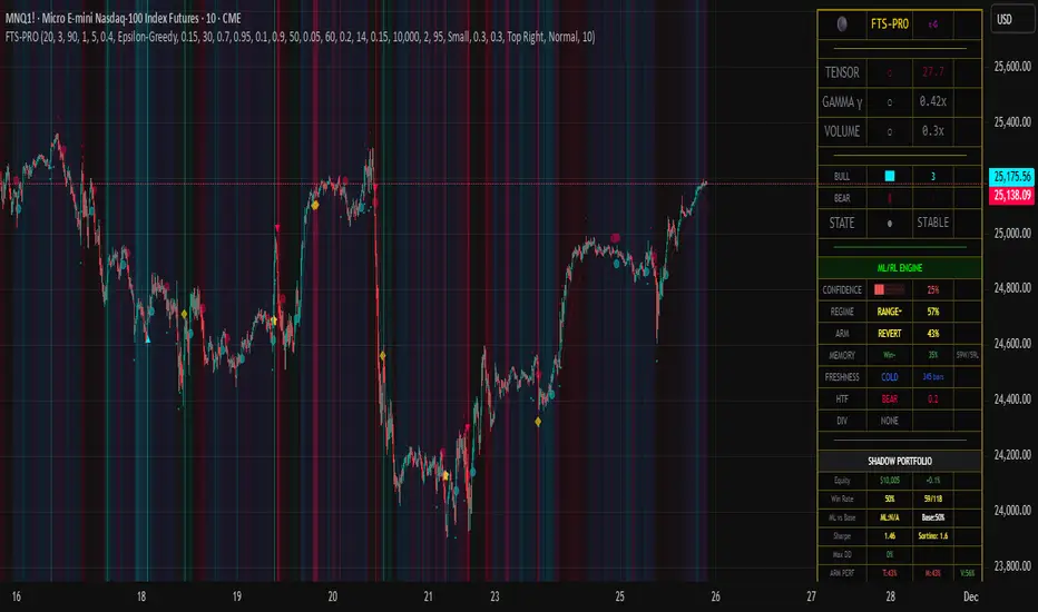
Contrarian Period High & LowContrarian Period High & Low
This indicator pairs nicely with the Contrarian 100 MA and can be located here:
Overview
The "Contrarian Period High & Low" indicator is a powerful technical analysis tool designed for traders seeking to identify key support and resistance levels and capitalize on contrarian trading opportunities. By tracking the highest highs and lowest lows over user-defined periods (Daily, Weekly, or Monthly), this indicator plots historical levels and generates buy and sell signals when price breaks these levels in a contrarian manner. A unique blue dot counter and action table enhance decision-making, making it ideal for swing traders, trend followers, and those trading forex, stocks, or cryptocurrencies. Optimized for daily charts, it can be adapted to other timeframes with proper testing.
How It Works
The indicator identifies the highest high and lowest low within a specified period (e.g., daily, weekly, or monthly) and draws horizontal lines for the previous period’s extremes on the chart. These levels act as dynamic support and resistance zones. Contrarian signals are generated when the price crosses below the previous period’s low (buy signal) or above the previous period’s high (sell signal), indicating potential reversals. A blue dot counter tracks consecutive buy signals, and a table displays the count and recommended action, helping traders decide whether to hold or flip positions.
Key Components
Period High/Low Levels: Tracks the highest high and lowest low for each period, plotting red lines for highs and green lines for lows from the bar where they occurred, extending for a user-defined length (default: 200 bars).
Contrarian Signals: Generates buy signals (blue circles) when price crosses below the previous period’s low and sell signals (white circles) when price crosses above the previous period’s high, designed to capture potential reversals.
Blue Dot Tracker: Counts consecutive buy signals (“blue dots”). If three or more occur, it suggests a stronger trend, with the table recommending whether to “Hold Investment” or “Flip Investment.”
Action Table: A 2x2 table in the bottom-right corner displays the blue dot count and action (“Hold Investment” if count ≥ 4, else “Flip Investment”) for quick reference.
Mathematical Concepts
Period Detection: Uses an approximate bar count to define periods (1 bar for Daily, 5 bars for Weekly, 20 bars for Monthly on a daily chart). When a new period starts, the previous period’s high/low is finalized and plotted.
High/Low Tracking:
Highest high (periodHigh) and lowest low (periodLow) are updated within the period.
Lines are drawn at these levels when the period ends, starting from the bar where the extreme occurred (periodHighBar, periodLowBar).
Signal Logic:
Buy signal: ta.crossunder(close , prevPeriodLow) and not lowBroken and barstate.isconfirmed
Sell signal: ta.crossover(close , prevPeriodHigh) and not highBroken and barstate.isconfirmed
Flags (highBroken, lowBroken) prevent multiple signals for the same level within a period.
Blue Dot Counter: Increments on each buy signal, resets on a sell signal or if price exceeds the entry price after three or more buy signals.
Entry and Exit Rules
Buy Signal (Blue Circle): Triggered when the price crosses below the previous period’s low, suggesting a potential oversold condition and buying opportunity. The signal appears as a blue circle below the price bar.
Sell Signal (White Circle): Triggered when the price crosses above the previous period’s high, indicating a potential overbought condition and selling opportunity. The signal appears as a white circle above the price bar.
Blue Dot Tracker:
Increments blueDotCount on each buy signal and sets an entryPrice on the first buy.
Resets on a sell signal or if price exceeds entryPrice after three or more buy signals.
If blueDotCount >= 3, the table suggests holding; if >= 4, it reinforces “Hold Investment.”
Exit Rules: Exit a buy position on a sell signal or when price exceeds the entry price after three or more buy signals. Combine with other tools (e.g., trendlines, support/resistance) for additional confirmation. Always apply proper risk management.
Recommended Usage
The "Contrarian Period High & Low" indicator is optimized for daily charts but can be adapted to other timeframes (e.g., 1H, 4H) with adjustments to the period bar count. It excels in markets with clear support/resistance levels and potential reversal zones. Traders should:
Backtest the indicator on their chosen asset and timeframe to validate signal reliability.
Combine with other technical tools (e.g., moving averages, Fibonacci levels) for stronger trade confirmation.
Adjust barsPerPeriod (e.g., ~120 bars for Weekly on hourly charts) based on the chart timeframe and market volatility.
Monitor the action table to guide position management based on blue dot counts.
Customization Options
Period Type: Choose between Daily, Weekly, or Monthly periods (default: Monthly).
Line Length: Set the length of high/low lines in bars (default: 200).
Show Highs/Lows: Toggle visibility of period high (red) and low (green) lines.
Max Lines to Keep: Limit the number of historical lines displayed (default: 10).
Hide Signals: Toggle buy/sell signal visibility for a cleaner chart.
Table Display: A fixed table in the bottom-right corner shows the blue dot count and action, with yellow (Hold) or green (Flip) backgrounds based on the count.
Why Use This Indicator?
The "Contrarian Period High & Low" indicator offers a unique blend of support/resistance visualization and contrarian signal generation, making it a versatile tool for identifying potential reversals. Its clear visual cues (lines and signals), blue dot tracker, and actionable table provide traders with an intuitive way to monitor market structure and manage trades. Whether you’re a beginner or an experienced trader, this indicator enhances your ability to spot key levels and time entries/exits effectively.
Tips for Users
Test the indicator thoroughly on your chosen market and timeframe to optimize settings (e.g., adjust barsPerPeriod for non-daily charts).
Use in conjunction with price action or other indicators for stronger trade setups.
Monitor the action table to decide whether to hold or flip positions based on blue dot counts.
Ensure your chart timeframe aligns with the selected period type (e.g., daily chart for Monthly periods).
Apply strict risk management to protect against false breakouts.
Happy trading with the Contrarian Period High & Low indicator! Share your feedback and strategies in the TradingView community!