Trend Breakout & Ratchet Stop System [Market Filter]Description:
This strategy implements a robust trend-following system designed to capture momentum moves while strictly managing downside risk through a multi-stage "Ratchet" exit mechanism and broad market filters.
It is designed for swing traders who want to align individual stock entries with the overall market direction.
How it works:
1. Market Regime Filters (The "Safety Check") Before taking any position, the strategy checks the health of the broader market to avoid "catching falling knives."
Broad Market Filter: By default, it checks NASDAQ:QQQ (adjustable). If the benchmark is trading below its SMA 200, the strategy assumes a Bear Market and suppresses all new long entries.
Volatility Filter (VIX): Uses CBOE:VIX to gauge fear. If the VIX is above a specific threshold (Default: 32), entries are paused, and existing positions can optionally be closed to preserve capital.
2. Entry Logic Entries are based on Momentum and Trend confirmation. A position is opened if filters are clear AND one of the following occurs:
Golden Cross: SMA 25 crosses over SMA 50.
SMA Breakouts: A "Three-Bar-Break" logic confirms a breakout above the SMA 50, 100, or 200 (price must establish itself above the moving average).
3. The "Ratchet" Exit System The exit logic evolves as the trade progresses, tightening risk like a ratchet:
Stage 0 (Initial Risk): Starts with a standard percentage Stop Loss from the entry price.
Stage 1 (Breakeven/Lock): Once the price rises by Profit Step 1 (e.g., +10%), the Stop Loss jumps to a tighter level and locks there. This secures the initial move.
Stage 2 (Trailing Mode): If the price continues to rise to Profit Step 2 (e.g., +15%), the Stop Loss converts into a dynamic Trailing Stop relative to the Highest High. This allows the trade to run as long as the trend persists.
Additional Exits:
Dead Cross: Closes position if SMA 25 crosses under SMA 50.
VIX Panic: Emergency exit if volatility spikes above the threshold.
Settings & Customization:
SMAs: Adjustable lengths for all Moving Averages.
Filters: Toggle Market/VIX filters on/off and choose your benchmark ticker (e.g., SPY or QQQ).
Risk Management: Fully customizable percentages for the Ratchet steps (Initial SL, Stage 1 Trigger, Trailing distance).
Penunjuk dan strategi

Elite Commodities AIThe Elite Commodities AI indicator provides a comprehensive analytical framework designed specifically for commodities trading. It combines multiple technical components to assess price action within the unique characteristics of commodity markets.
The indicator incorporates the following key elements:
Multi-timeframe RSI analysis across the primary timeframe, 4-hour, and daily periods
Multiple exponential moving averages (fast, slow, and trend) to establish directional context
Volume rate analysis measuring current volume relative to recent average volume
Bollinger Band width analysis to identify periods of volatility contraction
True Range volatility expressed as a percentage of price
The indicator evaluates the interaction between momentum, trend structure, volume participation, and volatility dynamics, which are particularly significant in commodities markets due to their sensitivity to changes in supply-demand fundamentals and large institutional order flow.
By combining these analytical components, the indicator provides a layered assessment of price behavior that captures the interplay between trend development, momentum characteristics, participation levels, and volatility compression—key factors that drive commodity market movements.
This approach enables traders to identify significant price action within the context of prevailing market structure, making it suitable for analyzing both directional trends and consolidation periods that are common in commodity price behavior.2.2s

Elite Bond Market AIDescription:
The Elite Bond Market AI indicator provides a comprehensive analytical framework specifically designed for bond market price action. The indicator combines multiple technical components including multi-timeframe RSI analysis, moving average relationships, volume dynamics, and volatility measurements to identify significant price behavior within the unique characteristics of bond market trading.
The indicator incorporates:
Multi-timeframe RSI evaluation across primary, 4-hour, and daily timeframes
Fast, slow, and trend exponential moving averages for directional context
Volume rate analysis relative to recent average volume
Bollinger Band width measurement for volatility contraction assessment
True Range volatility normalized as a percentage of price
This combination provides a layered analytical approach that captures the interplay between momentum, trend structure, participation levels, and volatility compression—key factors in bond market price discovery and directional moves.

Kira EMA9 EMA21 VWAP ZONES//@version=5
indicator("Kira EMA9 EMA21 VWAP ZONES", overlay=true)
// === EMAs ===
ema9 = ta.ema(close, 9)
ema21 = ta.ema(close, 21)
// === VWAP ===
vwapLine = ta.vwap(hlc3)
// === CONDITIONS ===
isBuy = ema9 > ema21 and close > vwapLine
isSell = ema9 < ema21 and close < vwapLine
noTrade = not isBuy and not isSell
// === PLOTS ===
plot(ema9, color=color.green, linewidth=2)
plot(ema21, color=color.red, linewidth=2)
plot(vwapLine, color=color.blue, linewidth=2)
// === BACKGROUND ZONES ===
bgcolor(isBuy ? color.new(color.green, 85) :
isSell ? color.new(color.red, 85) :
color.new(color.gray, 85))
// === BUY / SELL ARROWS EVERY BAR ===
plotshape(isBuy, title="BUY", style=shape.triangleup,
location=location.belowbar,
color=color.green, size=size.tiny)
plotshape(isSell, title="SELL", style=shape.triangledown,
location=location.abovebar,
color=color.red, size=size.tiny)
// === ALERTS ===
alertcondition(isBuy, title="BUY ZONE ACTIVE",
message="BUY zone active on {{ticker}}")
alertcondition(isSell, title="SELL ZONE ACTIVE",
message="SELL zone active on {{ticker}}")

Zone Levels (Range + ZoneHeight)This is a Template for drawing out zones from one ankerpoint zone.Just mark out the distance from one leveledge to the next and it will give you infinte more zoneedges in the same distance. You can also adjust the zone height if wanted (i used 10 as example).
I hope youll enjoy it
AJ

Local Watchlist Gauge v6The Local Watchlist Gauge displays a compact monitoring table for a user-defined list of symbols, showing their current trend status and performance relative to their 52-week high.
The indicator presents a table that simultaneously tracks multiple symbols and displays:
• Trend direction for each symbol, determined by whether the closing price is above or below a user-defined moving average
• Percentage distance from the 52-week high, providing a clear measure of recent performance relative to the yearly peak
Each symbol is displayed with:
Trend indicator showing whether the symbol is in an uptrend (above moving average) or downtrend (below moving average)
Distance from 52-week high expressed as a percentage, with color coding to indicate proximity to recent highs
Green indicates symbols trading within 5% of their 52-week high, orange indicates symbols between 5% and 20% below their 52-week high, and red indicates symbols trading more than 20% below their 52-week high.
The table provides an at-a-glance summary of the trend status and relative performance of all symbols in the specified watchlist, allowing users to quickly identify which instruments are maintaining trend strength near their recent highs and which have experienced significant pullbacks from their yearly peaks.

Dynamic Ratchet Trend Strategy [VIX Filter]Overview This strategy is a long-only trend-following system designed to capture major market moves while strictly managing downside risk through a state-machine based "Ratchet" exit logic. It incorporates a volatility filter using the CBOE VIX index to stay out of (or exit) the market during high-stress environments.
Key Features
1. Multi-Condition Entries The strategy looks for momentum shifts and trend breakouts using four Simple Moving Averages (25, 50, 100, 200).
Momentum Cross: SMA 25 crossover above SMA 50.
Trend Breakouts: A specific "3-Bar Breakout" logic above the SMA 50, 100, or 200. This requires the price to hold above the SMA for 3 consecutive bars after being below it, reducing false signals compared to simple closes.
2. VIX Volatility Filter Before entering any trade, the script checks the CBOE:VIX.
Filter: If VIX is above the threshold (default 32), new entries are blocked.
Panic Exit: If you are in a position and the VIX spikes above the threshold, the strategy executes an immediate "Panic Exit" to preserve capital during market crashes.
3. The "Ratchet" Exit System (3 Stages) Unlike a standard trailing stop, this strategy uses a 3-stage dynamic exit mechanism that tightens as profits grow:
Stage 0 (Initial Risk): Standard percentage-based Stop Loss from the entry price.
Stage 1 (The Lock-In): Triggered when profit hits 10% (configurable).
Unique Logic: Instead of trailing from the highest high, the stop is calculated based on the price at the exact moment this stage was triggered. It "steps up" once and holds, securing the initial move without being prematurely stopped out by normal volatility.
Stage 2 (Trailing Mode): Triggered when profit hits 15% (configurable).
The strategy switches to a classic Trailing Stop, following the percentage distance from the Highest High.
4. Emergency Backup A "Dead Cross" (SMA 25 crossing under SMA 50) acts as a final fail-safe to close positions if the trend reverses completely before hitting a stop.
Settings & Inputs
SMAs: Customize the lengths for all four moving averages.
VIX Filter: Toggle the filter on/off and set the panic threshold.
Exit Logic: Fully customizable percentages for Initial SL, Stage 1 Trigger/Distance, and Stage 2 Trigger/Trailing Distance.
Disclaimer This script is for educational purposes only. Past performance is not indicative of future results. Always manage your risk appropriately.

Granville 8-Rule Engine — v6Description:
The Granville 8-Rule Engine systematically implements Joseph Granville's eight original trading rules, which provide a comprehensive framework for interpreting price action relative to a moving average to identify genuine trend changes and avoid false signals.
Granville's methodology focuses on the critical relationship between price movement and the direction of the moving average, recognizing that valid trend changes and continuations exhibit specific behavioral patterns while false breakouts and reversals show characteristic divergences.
The indicator evaluates all eight of Granville's rules and assigns a composite score based on their fulfillment:
Bullish Rules:
Rule 1: Price crosses above a rising moving average (+3 points)
Rule 2: Price remains above a rising moving average after testing support (+2 points)
Rule 3: Price remains above a rising moving average after penetrating below it (+1 point)
Rule 4: Moving average changes from declining to rising (+1 point)
Bearish Rules:
Rule 5: Price crosses below a declining moving average (-3 points)
Rule 6: Price remains below a declining moving average after testing resistance (-2 points)
Rule 7: Price remains below a declining moving average after penetrating above it (-1 point)
The indicator incorporates volume confirmation by adding or subtracting additional points when significant volume accompanies the fulfillment of bullish or bearish rules, respectively.
A buy signal is generated when the composite score reaches +4 or higher, indicating multiple bullish rules are simultaneously satisfied. A sell signal is generated when the score reaches -4 or lower, indicating multiple bearish rules are in effect.
This systematic approach filters out many false breakout and whipsaw signals by requiring multiple confirmatory conditions rather than relying on simple moving average crossovers. The scoring mechanism provides a quantitative measure of the strength of the prevailing trend relationship, enabling traders to distinguish between genuine trend development and deceptive price movements that fail to confirm with the moving average direction.
The Granville 8-Rule Engine provides a disciplined, rule-based method for determining whether price movements represent valid trend continuation, genuine trend reversal, or potentially misleading counter-trend activity that is likely to fail. By requiring multiple confirmatory conditions from Granville's established rules, the indicator helps traders avoid premature entries and provides higher-probability signals for participating in sustained trend movements.

Moving Average 13 Exponential//@version=6
indicator(title="Moving Average 13 Exponential", shorttitle="EMA", overlay=true, timeframe="", timeframe_gaps=true)
len = input.int(9, minval=1, title="Length")
src = input(close, title="Source")
offset = input.int(title="Offset", defval=0, minval=-500, maxval=500, display = display.data_window)
out = ta.ema(src, len)
plot(out, title="EMA", color=color.yellow, offset=offset)
// Smoothing MA inputs
GRP = "Smoothing"
TT_BB = "Only applies when 'SMA + Bollinger Bands' is selected. Determines the distance between the SMA and the bands."
maTypeInput = input.string("None", "Type", options = , group = GRP, display = display.data_window)
var isBB = maTypeInput == "SMA + Bollinger Bands"
maLengthInput = input.int(14, "Length", group = GRP, display = display.data_window, active = maTypeInput != "None")
bbMultInput = input.float(2.0, "BB StdDev", minval = 0.001, maxval = 50, step = 0.5, tooltip = TT_BB, group = GRP, display = display.data_window, active = isBB)
var enableMA = maTypeInput != "None"
// Smoothing MA Calculation
ma(source, length, MAtype) =>
switch MAtype
"SMA" => ta.sma(source, length)
"SMA + Bollinger Bands" => ta.sma(source, length)
"EMA" => ta.ema(source, length)
"SMMA (RMA)" => ta.rma(source, length)
"WMA" => ta.wma(source, length)
"VWMA" => ta.vwma(source, length)
// Smoothing MA plots
smoothingMA = enableMA ? ma(out, maLengthInput, maTypeInput) : na
smoothingStDev = isBB ? ta.stdev(out, maLengthInput) * bbMultInput : na
plot(smoothingMA, "EMA-based MA", color=color.yellow, display = enableMA ? display.all : display.none, editable = enableMA)
bbUpperBand = plot(smoothingMA + smoothingStDev, title = "Upper Bollinger Band", color=color.green, display = isBB ? display.all : display.none, editable = isBB)
bbLowerBand = plot(smoothingMA - smoothingStDev, title = "Lower Bollinger Band", color=color.green, display = isBB ? display.all : display.none, editable = isBB)
fill(bbUpperBand, bbLowerBand, color= isBB ? color.new(color.green, 90) : na, title="Bollinger Bands Background Fill", display = isBB ? display.all : display.none, editable = isBB)

Volumen con línea promedio//@version=6
indicator("Volumen con línea promedio", overlay=false)
periodo = input.int(20, title="Período de media")
volumen = volume
mediaVolumen = ta.sma(volumen, periodo)
colorBarra = volumen > mediaVolumen ? color.green : color.red
plot(volumen, title="Volumen", style=plot.style_columns, color=colorBarra)
plot(mediaVolumen, title="Línea promedio", color=color.orange, linewidth=2, style=plot.style_line)

Smart Money Toolkit - PD Engine Bias Map [KedArc Quant]Description
Smart Money is an advanced multi-layer Smart Money Concepts framework that automatically detects structure shifts, premium-discount zones, and institutional order flow.
It is built around the PD Engine, which calculates the midpoint of the most recent market swing and dynamically determines BUY or SELL bias based on where current price trades relative to that equilibrium. This toolkit visualizes structure, order blocks, and bias context in one clean map, giving traders an institutional-grade view without unnecessary signal clutter.
Why It Is Unique
- All CHoCH, BOS, Order Block, FVG, and PD logic are coded from scratch.
- Uses true equilibrium (50 percent PD midpoint) for dynamic bias.
- Optimized for stability and non-repainting behavior.
- Designed for clarity with minimal, performance-safe visuals.
Entry and Exit Logic (Discretionary Framework)
- This toolkit is not a signal generator. It provides market context that guides discretionary trading.
BUY Bias (Discount Zone)
- Price trades below PD Mid: the market is in discount.
- Wait for a bullish CHoCH or reaction from a demand OB or FVG before buying.
- Target 1 = PD Mid. Target 2 = next opposite OB or FVG.
SELL Bias (Premium Zone)
- Price trades above PD Mid: the market is in premium.
- Wait for a bearish CHoCH or reaction from a supply OB or FVG before shorting.
- Target 1 = PD Mid. Target 2 = next opposite OB or FVG.
Institutional concept sequence: Bias → Structure Shift → Confirmation → Execution.
Input Configuration
Swing Sensitivity - Determines how far back to identify HH and LL pivots.
OB / FVG Detection - Toggles visual Order Block or Fair Value Gap zones.
PD Engine - Shows PD midpoint line, zone shading, and bias table.
Multi-TF Bias Sync - Optionally reads a higher timeframe bias for confirmation.
Color Themes - Switch between light, dark, or institutional palettes.
Formula / Logic Summary
Concept Formula
PD Mid (Equilibrium) (Recent Swing High + Recent Swing Low) / 2
BUY Bias close < PD Mid
SELL Bias close > PD Mid
CHoCH / BOS Pivot-based structure reversal: HH→LL or LL→HH
Order Block Last bullish or bearish candle before displacement.
FVG Gap between prior candle high/low and next candle range.
These formulas follow the structure used in institutional Smart Money Concepts.
How It Helps Traders
- Shows institutional premium and discount zones visually.
- Defines clear directional bias before entry.
- Combines structure, order blocks, FVG, and equilibrium in one layout.
- Works on any timeframe or asset.
- Prevents emotional trades by giving objective bias context.
Glossary
PD Mid Midpoint between recent swing high and low (market fair value).
Premium Zone Price above PD Mid; sellers control.
Discount Zone Price below PD Mid; buyers control.
CHoCH Change of Character, first reversal signal.
BOS Break of Structure, trend continuation confirmation.
OB Order Block, last institutional candle before move.
FVG Fair Value Gap, price imbalance often revisited.
FAQ
Q: Is this a signal indicator?
A: No. It is a contextual framework that supports manual decision-making.
Q: Does it repaint?
A: No. All structure logic is confirmed on bar close.
Q: Does it work on all markets?
A: Yes. It is purely price-based and timeframe independent.
Q: When does bias change?
A: Only after a new confirmed swing high or low.
Q: Can it be backtested?
A: You can build strategies on top of this context using your own entry and exit rules.
Disclaimer
This script is provided for educational purposes only.
It is not financial advice.
Trading carries risk. Past performance does not guarantee future results.
Use proper risk management and test on demo accounts before applying to live markets.

Ratchet Exit Trend Strategy with VIX FilterThis strategy is a trend-following system designed specifically for volatile markets. Instead of focusing solely on the "perfect entry," this script emphasizes intelligent trade management using a custom **"Ratchet Exit System."**
Additionally, it integrates a volatility filter based on the CBOE Volatility Index (VIX) to minimize risk during extreme market phases.
### 🎯 The Concept: Ratchet Exit
The "Ratchet" system operates like a mechanical ratchet tool: the Stop Loss can only move in one direction (up, for long trades) and "locks" into specific stages. The goal is to give the trade "room to breathe" initially to avoid being stopped out by noise, then aggressively reduce risk as the trade moves into profit.
The exit logic moves through 3 distinct phases:
1. **Phase 0 (Initial Risk):** At the start of the trade, a wide Stop Loss is set (Default: 10%) to tolerate normal market volatility.
2. **Phase 1 (Risk Reduction):** Once the trade reaches a specific floating profit (Default: +10%), the Stop Loss is raised and "pinned" to a fixed value (Default: -8% from entry). This drastically reduces risk while keeping the trade alive.
3. **Phase 2 (Trailing Mode):** If the trend extends to a higher profit zone (Default: +15%), the Stop switches to a dynamic Trailing Mode. It follows the **Highest High** at a fixed percentage distance (Default: 8%).
### 🛡️ VIX Filter & Panic Exit
High volatility is often the enemy of trend-following strategies.
* **Entry Filter:** The system will not enter new positions if the VIX is above a user-defined threshold (Default: 32). This helps avoid entering "falling knife" markets.
* **Panic Exit:** If the VIX spikes above the threshold (32) while a trade is open, the position is closed immediately to protect capital (Emergency Exit).
### 📈 Entry Signals
The strategy trades **LONG only** and uses Simple Moving Averages (SMAs) to identify trends:
* **Golden Cross:** SMA 25 crosses over SMA 50.
* **3-Bar Breakouts:** A confirmation logic where the price must close above the SMA 50, 100, or 200 for 3 consecutive bars.
### ⚙️ Settings (Inputs)
All parameters are fully customizable via the settings menu:
* **SMAs:** Lengths for the trend indicators (Default: 25, 50, 100, 200).
* **VIX Filter:** Toggle the filter on/off and adjust the panic threshold.
* **Ratchet Settings:** Percentages for Initial Stop, Trigger Levels for Stages 1 & 2, and the Trailing Distance.
### ⚠️ Technical Note & Risk Warning
This script uses `request.security` to fetch VIX data. Please ensure you understand the risks associated with trading leveraged or volatile assets. Past performance is not indicative of future results.

Best Entry Swing MASTER v3 PUBLIC (S.S)Strategy Description (English)
Best Entry Swing MASTER v3 – Quality Mode
The Best Entry Swing MASTER v3 is a structured swing trading and trend-following strategy designed to identify high-probability long and short entries during directional markets.
It combines three core setup types commonly used by momentum and breakout traders:
Breakout (BO)
Pullback Reversal (PB)
Volatility Contraction Pattern (VCP)
The strategy applies multiple layers of confirmation, including multi-EMA trend structure, volatility contraction, volume filters, and an optional market regime filter.
It is suitable for swing trading on higher timeframes (4H, Daily), as well as medium-term trend continuation setups.
Core Concepts
1. Trend Structure
A trend is considered valid when:
Uptrend: Price > EMA20 > EMA50 > EMA100
Downtrend: Price < EMA20 < EMA50 < EMA100
In addition, a simple but effective trend-strength metric is calculated using the percentage spread between EMA20 and EMA100.
This helps avoid signals during sideways or low-volatility environments.
2. Market Regime Filter
The market environment is determined using a higher timeframe benchmark (default: SPY on Daily).
Only long trades are allowed in bullish market conditions
Only short trades in bearish conditions
This significantly reduces false signals in counter-trend conditions.
Entry Logic
Breakout (BO)
A long breakout triggers when:
Price closes above the highest high of the lookback period
Volume exceeds its 20-period average
Trend and market regime confirm
(Optional A+ mode): true volatility contraction is required
Similar logic applies for short breakdowns.
Pullback (PB)
A pullback entry triggers after:
At least two corrective candles
A strong reversal candle (close above previous high for long)
Volume confirmation
Price interacts with EMA20
This structure models classical trend-reentry conditions.
Volatility Contraction Pattern (VCP)
A VCP entry triggers when:
True range contracts over multiple bars
Price holds near the breakout zone
Volume contracts
Trend and market regime are aligned
This setup aims to capture explosive continuation moves.
Quality Modes
The strategy offers two modes:
Balanced Mode
Moderate signal frequency
Broader trend-strength allowance
Suitable for more active traders
A+ Only Mode
Strict confirmation requirements
Only high-quality setups with multiple confluences
Designed to avoid low-probability trades entirely
Risk Management
Risk is managed using an ATR-based stop and target:
Long SL = Close − ATR × 1.5
Long TP = Close + ATR × 3
(Equivalent logic for short positions)
This provides a balanced reward-to-risk profile and avoids overly tight stops.
Early Entry Signals (Optional)
The script offers optional “Early Entry” markers that highlight when a setup is forming but not yet confirmed.
These are not entry signals and are disabled by default for public use.
Intended Use
This strategy is designed for:
Swing trading
Momentum continuation
Trend-following
Multi-day to multi-week trades
It performs best on:
4H
Daily
High-liquidity equities, indices, and futures
Disclaimer
This script is intended for educational and research purposes.
Past performance does not guarantee future results.
Always backtest thoroughly and use appropriate risk management.

Z-EMA Fusion BandsDesigned with crypto markets in mind, particularly Bitcoin , it builds on the concept that the 1-Week 50 EMA often serves as a long-term bull/bear market threshold — an area where institutional bias, momentum shifts, and cyclical rotations tend to occur.
🔹 Core Components & Synergies:
1. 1W 50 EMA (Higher Timeframe)
- This EMA is calculated on a weekly timeframe, regardless of your current chart.
- In crypto, price above the 1W 50 EMA typically aligns with long-term bull market phases, while extended periods below can signify bearish macro structure.
- The slope of the EMA is also analyzed to add directional confidence to trend strength.
2. ±1 Standard Deviation Bands
- Surrounding the 50 EMA, these bands visualize normal price dispersion relative to trend.
- When price consistently hugs or breaks outside these bands, it often reflects market expansion, volatility events, or mean-reversion opportunity.
3. Z-Score Gradient Fill
- The area between the bands is filled using a Z-score-based gradient, which dynamically adjusts color based on how far price is from the EMA (in terms of standard deviations).
- Color shifts from aqua (near EMA) to fuchsia (far from EMA) help you spot price compression, equilibrium, or overextension at a glance.
- The fill also uses transparency scaling, making it fade as price stretches further, emphasizing the core structure.
4. Directional EMA Coloring
- The EMA line itself is colored based on:
- The slope of the EMA (rising/falling)
- Whether the HTF candle is bullish or bearish
- This provides intuitive color-coded confirmation of momentum alignment or potential exhaustion.
5. Price/EMA Divergence Detection
- The script detects bullish and bearish divergence between price and the EMA (rather than using a traditional oscillator).
- Bullish Divergence: Price makes a lower low, EMA makes a higher low.
- Bearish Divergence: Price makes a higher high, EMA makes a lower high.
- These signals often mark transitional zones where momentum fades before a trend reversal or correction.
📊 Suggested Uses:
🔸 Swing and Position Trading:
- Use the 1W 50 EMA as a macro-trend anchor.
- Stay long-biased when price is above with positive slope, and short-biased when below.
- Consider entries near band edges for mean-reversion plays, especially if confluence forms with divergence signals.
🔸 Volatility-Based Filtering:
- Use the Z-score fill to identify volatility compression (near EMA) or expansion (edge of bands).
- Combine this with breakout strategies or dynamic position sizing.
🔸 Divergence Confirmation:
- Combine divergence markers with HTF EMA slope for high-probability setups.
- Bullish div + EMA flattening/rising can signal the start of accumulation after a macro dip.
🔸 Multi-Timeframe Analysis:
- Works well as a structural overlay on intraday charts (1H, 4H, 1D).
- Use this indicator to track long-term bias while executing lower timeframe trades.
⚠️ Disclaimer:
This indicator is designed for educational and informational purposes only. It does not constitute financial advice or a recommendation to buy or sell any asset.
Always use proper risk management, and combine with your own analysis, tools, and strategy. Performance in past market conditions does not guarantee future results.

Simple Price ChannelSimple Price Channel
This indicator plots a basic volatility-based channel around a moving average.
Features:
Midline using Simple Moving Average (SMA)
Upper & lower bands using ATR or true range
Channel fill for easy trend visualisation
This script is designed for educational and analytical purposes only.
It does not provide signals, alerts, or financial advice.

Vibha Jha TQQQ Clean Buy/Sell📈 Vibha Jha TEQQ Hybrid Strategy — Buy/Sell Signals
This script replicates the high-performance buy/sell methodology of Vibha Jha, one of the top money-manager performers in the U.S. Investing Championship (USIC). Her hybrid system generated triple-digit returns in both 2020 and 2021, and strong follow-up performance in 2023–2024 through a strict, rules-based combination of:
✔ CANSLIM-style market leadership tracking
✔ Position-trading fundamentals
✔ Rules-based swing trading using TQQQ/QQQ
✔ Tight entries & disciplined sells
✔ Market-timed exposure based on follow-through days, 21-EMA, and distribution clusters
🚀 What This Indicator Does
This indicator plots clean BUY and SELL signals based on Vibha’s core rule set:
BUY Signals
Three consecutive higher highs AND higher lows (her famous “3-day up” rule)
Strong up-day with rising volume
Designed to catch early trend reversals and early-stage rally attempts
SELL Signals
Two closes below the 21-day EMA
Three consecutive down days
Distribution cluster (4+ distribution days in the last 6 bars)
Captures exhaustion, weakening trend, and institutional selling
🧠 Why This Works
Vibha’s system is built on the reality that:
🔹 Markets give early warning before reversing
🔹 Momentum shifts appear before fundamentals
🔹 Distribution clusters precede pullbacks
🔹 3-day up patterns often kick off powerful rallies
🔹 TQQQ/QQQ respond clearly to technical signals
This indicator applies those insights directly to your chart—stocks, crypto, indices, or leveraged ETFs.

Vibha Jha TQQQ Clean Buy/SellVibha Jha TQQQ buy sell strategy its the best we use it to see when to enter and exit a trade especially TQQQ I want to publish it

P&F Label Overlay🧙 The Wizard's Challenge: P&F Label Overlay on Your Chart
This is a custom Pine Script indicator designed to overlay the classic Point & Figure (P&F) pattern directly onto your standard candlestick or bar chart. While Pine Script offers built-in, dedicated P&F charts, this indicator was created as a challenging and experimental project to satisfy the goal of visualizing the P&F X's and O's directly on the price bars.
❶. How to Use This Code on TradingView
1. Copy the Code: Copy the entire Pine Script code provided above.
2. Open Pine Editor: On TradingView, click the "Pine Editor" tab at the bottom of your chart.
3. Replace Content: Delete any existing code in the editor and paste this P&F script.
4. Add to Chart: Click the "Add to Chart" button (usually located near the top right of the Pine Editor).
5. Access Settings: The indicator, named "P&F Label Overlay: The Wizard's Challenge," will appear on your chart. You can click the gear icon ( ) next to its name on the chart to adjust the inputs.
❷. 🎛️ Key Settings & Customization (Inputs)
The indicator provides core P&F settings that you can customize to fit your analysis style:
✅ Enable Auto Box Size (Default: True): When enabled, the box size is automatically calculated as a percentage of the current price, making it dynamic.
・Auto Box Size Basis (%): Sets the percentage used to calculate the dynamic box size. (e.g., 2% of the price).
・Fixed Box Size (Price Units): When "Enable Auto Box Size" is disabled, this value is used as the static box size (e.g., a value of 5.0 for a $5 box).
・Reversal Count (Default: 3): This is the crucial P&F parameter (the Reversal Factor). It determines how many boxes the price must move in the opposite direction to trigger a column reversal (e.g., 3 means price must reverse by 3 \times \text{BOX\_SIZE}).
Calculation Source: Allows you to choose the price data used for calculations (e.g., close, hl2 (High/Low/2), etc.).
❸. 🎯 The Challenge: Why an Overlay?
This indicator represents an experimental and challenging endeavor made in collaboration with an AI. It stems from the strong desire to visualize P&F patterns overlaid on a conventional chart, which is not a native function in Pine Script's standard indicator plotting system.
・Leveraging Drawing Objects: The core of this challenge relies on cleverly using Pine Script's label.new() drawing objects to represent the "X" and "O" symbols. This is a highly non-standard way to draw a P&F chart, as it requires complex logic to manage the drawing coordinates, price levels, and column spacing on the time-based chart.
・The Current Status: We've successfully achieved the initial goal: visualizing the X and O patterns as an overlay. Achieving a perfectly aligned, full-featured P&F chart (where columns align precisely, and price rounding is fully consistent across all columns) is far more complex, but this code provides a strong foundation.
❹. 🛠️ Technical Highlights
Tick-Precision Rounding: The custom function f_roundToTick() is critical. It ensures that the calculated box size and the lastPrice are always rounded to the nearest minimum tick size (syminfo.mintick) of the asset. This maintains high precision and accuracy relative to the market's price movements.
・Column Indexing: The currentColumnIndex variable is used to simulate the horizontal movement of P&F columns by adding a fractional offset to the bar_index when drawing the labels. This is what makes the pattern appear as distinct columns.
・Garbage Collection: The activeLabels array and the MAX_LABELS limit ensure that old labels are deleted (label.delete()) as new ones are drawn. This is a crucial performance optimization to prevent TradingView's label limit (500) from being exceeded and to maintain a smooth experience.
❺. 🚀 A Platform for Deep Customization
While TradingView's built-in indicators are excellent, every trader has their "personal best settings." View this code as a starting point for your own analytical environment. You can use it as a base to pursue deeper custom features, such as:
・Different drawing styles or colors based on momentum.
・Automated detection and signaling of specific P&F patterns (e.g., Double Top Buy, Triple Bottom Sell).
Please feel free to try it on your chart! We welcome any feedback you might have as we continue to refine this experimental overlay.
I do not speak English at all. Please understand that if you send me a message, I may not be able to reply, or my reply may have a different meaning. Thank you for your understanding.

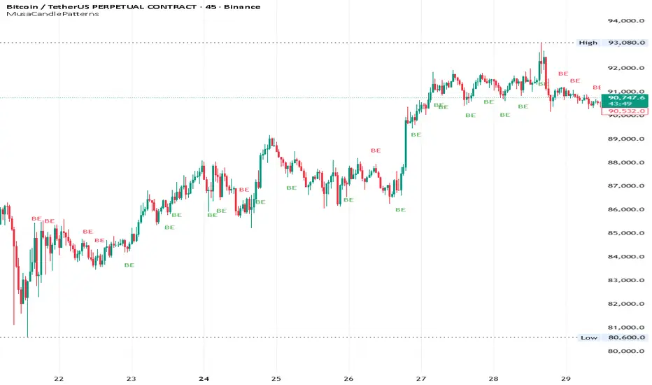
MusaCandlePatternsLibrary "MusaCandlePatterns"
Patterns is a Japanese candlestick pattern recognition Library for developers. Functions here within detect viable setups in a variety of popular patterns. Please note some patterns are without filters such as comparisons to average candle sizing, or trend detection to allow the author more freedom.
doji(dojiSize, dojiWickSize)
Detects "Doji" candle patterns
Parameters:
dojiSize (float) : (float) The relationship of body to candle size (ie. body is 5% of total candle size). Default is 5.0 (5%)
dojiWickSize (float) : (float) Maximum wick size comparative to the opposite wick. (eg. 2 = bottom wick must be less than or equal to 2x the top wick). Default is 2
Returns: (series bool) True when pattern detected
dLab(showLabel, labelColor, textColor)
Produces "Doji" identifier label
Parameters:
showLabel (bool) : (series bool) Shows label when input is true. Default is false
labelColor (color) : (series color) Color of the label border and arrow
textColor (color) : (series color) Text color
Returns: (label) A label visible at the chart level intended for the title pattern
bullEngulf(maxRejectWick, mustEngulfWick)
Detects "Bullish Engulfing" candle patterns
Parameters:
maxRejectWick (float) : (float) Maximum rejection wick size.
The maximum wick size as a percentge of body size allowable for a top wick on the resolution candle of the pattern. 0.0 disables the filter.
eg. 50 allows a top wick half the size of the body. Default is 0% (Disables wick detection).
mustEngulfWick (bool) : (bool) input to only detect setups that close above the high prior effectively engulfing the candle in its entirety. Default is false
Returns: (series bool) True when pattern detected
bewLab(showLabel, labelColor, textColor)
Produces "Bullish Engulfing" identifier label
Parameters:
showLabel (bool) : (series bool) Shows label when input is true. Default is false
labelColor (color) : (series color) Color of the label border and arrow
textColor (color) : (series color) Text color
Returns: (label) A label visible at the chart level intended for the title pattern
bearEngulf(maxRejectWick, mustEngulfWick)
Detects "Bearish Engulfing" candle patterns
Parameters:
maxRejectWick (float) : (float) Maximum rejection wick size.
The maximum wick size as a percentge of body size allowable for a bottom wick on the resolution candle of the pattern. 0.0 disables the filter.
eg. 50 allows a botom wick half the size of the body. Default is 0% (Disables wick detection).
mustEngulfWick (bool) : (bool) Input to only detect setups that close below the low prior effectively engulfing the candle in its entirety. Default is false
Returns: (series bool) True when pattern detected
bebLab(showLabel, labelColor, textColor)
Produces "Bearish Engulfing" identifier label
Parameters:
showLabel (bool) : (series bool) Shows label when input is true. Default is false
labelColor (color) : (series color) Color of the label border and arrow
textColor (color) : (series color) Text color
Returns: (label) A label visible at the chart level intended for the title pattern
hammer(ratio, shadowPercent)
Detects "Hammer" candle patterns
Parameters:
ratio (float) : (float) The relationship of body to candle size (ie. body is 33% of total candle size). Default is 33%.
shadowPercent (float) : (float) The maximum allowable top wick size as a percentage of body size. Default is 5%.
Returns: (series bool) True when pattern detected
hLab(showLabel, labelColor, textColor)
Produces "Hammer" identifier label
Parameters:
showLabel (bool) : (series bool) Shows label when input is true. Default is false
labelColor (color) : (series color) Color of the label border and arrow
textColor (color) : (series color) Text color
Returns: (label) A label visible at the chart level intended for the title pattern
star(ratio, shadowPercent)
Detects "Star" candle patterns
Parameters:
ratio (float) : (float) The relationship of body to candle size (ie. body is 33% of total candle size). Default is 33%.
shadowPercent (float) : (float) The maximum allowable bottom wick size as a percentage of body size. Default is 5%.
Returns: (series bool) True when pattern detected
ssLab(showLabel, labelColor, textColor)
Produces "Star" identifier label
Parameters:
showLabel (bool) : (series bool) Shows label when input is true. Default is false
labelColor (color) : (series color) Color of the label border and arrow
textColor (color) : (series color) Text color
Returns: (label) A label visible at the chart level intended for the title pattern
dragonflyDoji()
Detects "Dragonfly Doji" candle patterns
Returns: (series bool) True when pattern detected
ddLab(showLabel, labelColor, textColor)
Produces "Dragonfly Doji" identifier label
Parameters:
showLabel (bool) : (series bool) Shows label when input is true. Default is false
labelColor (color) : (series color) Color of the label border and arrow
textColor (color)
Returns: (label) A label visible at the chart level intended for the title pattern
gravestoneDoji()
Detects "Gravestone Doji" candle patterns
Returns: (series bool) True when pattern detected
gdLab(showLabel, labelColor, textColor)
Produces "Gravestone Doji" identifier label
Parameters:
showLabel (bool) : (series bool) Shows label when input is true. Default is false
labelColor (color) : (series color) Color of the label border and arrow
textColor (color) : (series color) Text color
Returns: (label) A label visible at the chart level intended for the title pattern
tweezerBottom(closeUpperHalf)
Detects "Tweezer Bottom" candle patterns
Parameters:
closeUpperHalf (bool) : (bool) input to only detect setups that close above the mid-point of the candle prior increasing its bullish tendancy. Default is false
Returns: (series bool) True when pattern detected
tbLab(showLabel, labelColor, textColor)
Produces "Tweezer Bottom" identifier label
Parameters:
showLabel (bool) : (series bool) Shows label when input is true. Default is false
labelColor (color) : (series color) Color of the label border and arrow
textColor (color) : (series color) Text color
Returns: (label) A label visible at the chart level intended for the title pattern
tweezerTop(closeLowerHalf)
Detects "TweezerTop" candle patterns
Parameters:
closeLowerHalf (bool) : (bool) input to only detect setups that close below the mid-point of the candle prior increasing its bearish tendancy. Default is false
Returns: (series bool) True when pattern detected
ttLab(showLabel, labelColor, textColor)
Produces "TweezerTop" identifier label
Parameters:
showLabel (bool) : (series bool) Shows label when input is true. Default is false
labelColor (color) : (series color) Color of the label border and arrow
textColor (color) : (series color) Text color
Returns: (label) A label visible at the chart level intended for the title pattern
spinningTopBull(wickSize)
Detects "Bullish Spinning Top" candle patterns
Parameters:
wickSize (float) : (float) input to adjust detection of the size of the top wick/ bottom wick as a percent of total candle size. Default is 34%, which ensures the wicks are both larger than the body.
Returns: (series bool) True when pattern detected
stwLab(showLabel, labelColor, textColor)
Produces "Bullish Spinning Top" identifier label
Parameters:
showLabel (bool) : (series bool) Shows label when input is true. Default is false
labelColor (color) : (series color) Color of the label border and arrow
textColor (color) : (series color) Text color
Returns: (label) A label visible at the chart level intended for the title pattern
spinningTopBear(wickSize)
Detects "Bearish Spinning Top" candle patterns
Parameters:
wickSize (float) : (float) input to adjust detection of the size of the top wick/ bottom wick as a percent of total candle size. Default is 34%, which ensures the wicks are both larger than the body.
Returns: (series bool) True when pattern detected
stbLab(showLabel, labelColor, textColor)
Produces "Bearish Spinning Top" identifier label
Parameters:
showLabel (bool) : (series bool) Shows label when input is true. Default is false
labelColor (color) : (series color) Color of the label border and arrow
textColor (color) : (series color) Text color
Returns: (label) A label visible at the chart level intended for the title pattern
spinningTop(wickSize)
Detects "Spinning Top" candle patterns
Parameters:
wickSize (float) : (float) input to adjust detection of the size of the top wick/ bottom wick as a percent of total candle size. Default is 34%, which ensures the wicks are both larger than the body.
Returns: (series bool) True when pattern detected
stLab(showLabel, labelColor, textColor)
Produces "Spinning Top" identifier label
Parameters:
showLabel (bool) : (series bool) Shows label when input is true. Default is false
labelColor (color) : (series color) Color of the label border and arrow
textColor (color) : (series color) Text color
Returns: (label) A label visible at the chart level intended for the title pattern
morningStar()
Detects "Bullish Morning Star" candle patterns
Returns: (series bool) True when pattern detected
msLab(showLabel, labelColor, textColor)
Produces "Bullish Morning Star" identifier label
Parameters:
showLabel (bool) : (series bool) Shows label when input is true. Default is false
labelColor (color) : (series color) Color of the label border and arrow
textColor (color) : (series color) Text color
Returns: (label) A label visible at the chart level intended for the title pattern
eveningStar()
Detects "Bearish Evening Star" candle patterns
Returns: (series bool) True when pattern detected
esLab(showLabel, labelColor, textColor)
Produces "Bearish Evening Star" identifier label
Parameters:
showLabel (bool) : (series bool) Shows label when input is true. Default is false
labelColor (color) : (series color) Color of the label border and arrow
textColor (color) : (series color) Text color
Returns: (label) A label visible at the chart level intended for the title pattern
haramiBull()
Detects "Bullish Harami" candle patterns
Returns: (series bool) True when pattern detected
hwLab(showLabel, labelColor, textColor)
Produces "Bullish Harami" identifier label
Parameters:
showLabel (bool) : (series bool) Shows label when input is true. Default is false
labelColor (color) : (series color) Color of the label border and arrow
textColor (color) : (series color) Text color
Returns: (label) A label visible at the chart level intended for the title pattern
haramiBear()
Detects "Bearish Harami" candle patterns
Returns: (series bool) True when pattern detected
hbLab(showLabel, labelColor, textColor)
Produces "Bearish Harami" identifier label
Parameters:
showLabel (bool) : (series bool) Shows label when input is true. Default is false
labelColor (color) : (series color) Color of the label border and arrow
textColor (color) : (series color) Text color
Returns: (label) A label visible at the chart level intended for the title pattern
haramiBullCross()
Detects "Bullish Harami Cross" candle patterns
Returns: (series bool) True when pattern detected
hcwLab(showLabel, labelColor, textColor)
Produces "Bullish Harami Cross" identifier label
Parameters:
showLabel (bool) : (series bool) Shows label when input is true. Default is false
labelColor (color) : (series color) Color of the label border and arrow
textColor (color) : (series color) Text color
Returns: (label) A label visible at the chart level intended for the title pattern
haramiBearCross()
Detects "Bearish Harami Cross" candle patterns
Returns: (series bool) True when pattern detected
hcbLab(showLabel, labelColor, textColor)
Produces "Bearish Harami Cross" identifier label
Parameters:
showLabel (bool) : (series bool) Shows label when input is true. Default is false
labelColor (color) : (series color) Color of the label border and arrow
textColor (color)
Returns: (label) A label visible at the chart level intended for the title pattern
marubullzu()
Detects "Bullish Marubozu" candle patterns
Returns: (series bool) True when pattern detected
mwLab(showLabel, labelColor, textColor)
Produces "Bullish Marubozu" identifier label
Parameters:
showLabel (bool) : (series bool) Shows label when input is true. Default is false
labelColor (color) : (series color) Color of the label border and arrow
textColor (color) : (series color) Text color
Returns: (label) A label visible at the chart level intended for the title pattern
marubearzu()
Detects "Bearish Marubozu" candle patterns
Returns: (series bool) True when pattern detected
mbLab(showLabel, labelColor, textColor)
Produces "Bearish Marubozu" identifier label
Parameters:
showLabel (bool) : (series bool) Shows label when input is true. Default is false
labelColor (color) : (series color) Color of the label border and arrow
textColor (color) : (series color) Text color
Returns: (label) A label visible at the chart level intended for the title pattern
abandonedBull()
Detects "Bullish Abandoned Baby" candle patterns
Returns: (series bool) True when pattern detected
abwLab(showLabel, labelColor, textColor)
Produces "Bullish Abandoned Baby" identifier label
Parameters:
showLabel (bool) : (series bool) Shows label when input is true. Default is false
labelColor (color) : (series color) Color of the label border and arrow
textColor (color) : (series color) Text color
Returns: (label) A label visible at the chart level intended for the title pattern
abandonedBear()
Detects "Bearish Abandoned Baby" candle patterns
Returns: (series bool) True when pattern detected
abbLab(showLabel, labelColor, textColor)
Produces "Bearish Abandoned Baby" identifier label
Parameters:
showLabel (bool) : (series bool) Shows label when input is true. Default is false
labelColor (color) : (series color) Color of the label border and arrow
textColor (color) : (series color) Text color
Returns: (label) A label visible at the chart level intended for the title pattern
piercing()
Detects "Piercing" candle patterns
Returns: (series bool) True when pattern detected
pLab(showLabel, labelColor, textColor)
Produces "Piercing" identifier label
Parameters:
showLabel (bool) : (series bool) Shows label when input is true. Default is false
labelColor (color) : (series color) Color of the label border and arrow
textColor (color) : (series color) Text color
Returns: (label) A label visible at the chart level intended for the title pattern
darkCloudCover()
Detects "Dark Cloud Cover" candle patterns
Returns: (series bool) True when pattern detected
dccLab(showLabel, labelColor, textColor)
Produces "Dark Cloud Cover" identifier label
Parameters:
showLabel (bool) : (series bool) Shows label when input is true. Default is false
labelColor (color) : (series color) Color of the label border and arrow
textColor (color) : (series color) Text color
Returns: (label) A label visible at the chart level intended for the title pattern
tasukiBull()
Detects "Upside Tasuki Gap" candle patterns
Returns: (series bool) True when pattern detected
utgLab(showLabel, labelColor, textColor)
Produces "Upside Tasuki Gap" identifier label
Parameters:
showLabel (bool) : (series bool) Shows label when input is true. Default is false
labelColor (color) : (series color) Color of the label border and arrow
textColor (color) : (series color) Text color
Returns: (label) A label visible at the chart level intended for the title pattern
tasukiBear()
Detects "Downside Tasuki Gap" candle patterns
Returns: (series bool) True when pattern detected
dtgLab(showLabel, labelColor, textColor)
Produces "Downside Tasuki Gap" identifier label
Parameters:
showLabel (bool) : (series bool) Shows label when input is true. Default is false
labelColor (color) : (series color) Color of the label border and arrow
textColor (color) : (series color) Text color
Returns: (label) A label visible at the chart level intended for the title pattern
risingThree()
Detects "Rising Three Methods" candle patterns
Returns: (series bool) True when pattern detected
rtmLab(showLabel, labelColor, textColor)
Produces "Rising Three Methods" identifier label
Parameters:
showLabel (bool) : (series bool) Shows label when input is true. Default is false
labelColor (color) : (series color) Color of the label border and arrow
textColor (color) : (series color) Text color
Returns: (label) A label visible at the chart level intended for the title pattern
fallingThree()
Detects "Falling Three Methods" candle patterns
Returns: (series bool) True when pattern detected
ftmLab(showLabel, labelColor, textColor)
Produces "Falling Three Methods" identifier label
Parameters:
showLabel (bool) : (series bool) Shows label when input is true. Default is false
labelColor (color) : (series color) Color of the label border and arrow
textColor (color) : (series color) Text color
Returns: (label) A label visible at the chart level intended for the title pattern
risingWindow()
Detects "Rising Window" candle patterns
Returns: (series bool) True when pattern detected
rwLab(showLabel, labelColor, textColor)
Produces "Rising Window" identifier label
Parameters:
showLabel (bool) : (series bool) Shows label when input is true. Default is false
labelColor (color) : (series color) Color of the label border and arrow
textColor (color) : (series color) Text color
Returns: (label) A label visible at the chart level intended for the title pattern
fallingWindow()
Detects "Falling Window" candle patterns
Returns: (series bool) True when pattern detected
fwLab(showLabel, labelColor, textColor)
Produces "Falling Window" identifier label
Parameters:
showLabel (bool) : (series bool) Shows label when input is true. Default is false
labelColor (color) : (series color) Color of the label border and arrow
textColor (color) : (series color) Text color
Returns: (label) A label visible at the chart level intended for the title pattern
kickingBull()
Detects "Bullish Kicking" candle patterns
Returns: (series bool) True when pattern detected
kwLab(showLabel, labelColor, textColor)
Produces "Bullish Kicking" identifier label
Parameters:
showLabel (bool) : (series bool) Shows label when input is true. Default is false
labelColor (color) : (series color) Color of the label border and arrow
textColor (color) : (series color) Text color
Returns: (label) A label visible at the chart level intended for the title pattern
kickingBear()
Detects "Bearish Kicking" candle patterns
Returns: (series bool) True when pattern detected
kbLab(showLabel, labelColor, textColor)
Produces "Bearish Kicking" identifier label
Parameters:
showLabel (bool) : (series bool) Shows label when input is true. Default is false
labelColor (color) : (series color) Color of the label border and arrow
textColor (color) : (series color) Text color
Returns: (label) A label visible at the chart level intended for the title pattern
lls(ratio)
Detects "Long Lower Shadow" candle patterns
Parameters:
ratio (float) : (float) A relationship of the lower wick to the overall candle size expressed as a percent. Default is 75%
Returns: (series bool) True when pattern detected
llsLab(showLabel, labelColor, textColor)
Produces "Long Lower Shadow" identifier label
Parameters:
showLabel (bool) : (series bool) Shows label when input is true. Default is false
labelColor (color) : (series color) Color of the label border and arrow
textColor (color) : (series color) Text color
Returns: (label) A label visible at the chart level intended for the title pattern
lus(ratio)
Detects "Long Upper Shadow" candle patterns
Parameters:
ratio (float) : (float) A relationship of the upper wick to the overall candle size expressed as a percent. Default is 75%
Returns: (series bool) True when pattern detected
lusLab(showLabel, labelColor, textColor)
Produces "Long Upper Shadow" identifier label
Parameters:
showLabel (bool) : (series bool) Shows label when input is true. Default is false
labelColor (color) : (series color) Color of the label border and arrow
textColor (color) : (series color) Text color
Returns: (label) A label visible at the chart level intended for the title pattern
bullNeck()
Detects "Bullish On Neck" candle patterns
Returns: (series bool) True when pattern detected
nwLab(showLabel, labelColor, textColor)
Produces "Bullish On Neck" identifier label
Parameters:
showLabel (bool) : (series bool) Shows label when input is true. Default is false
labelColor (color) : (series color) Color of the label border and arrow
textColor (color) : (series color) Text color
Returns: (label) A label visible at the chart level intended for the title pattern
bearNeck()
Detects "Bearish On Neck" candle patterns
Returns: (series bool) True when pattern detected
nbLab(showLabel, labelColor, textColor)
Produces "Bearish On Neck" identifier label
Parameters:
showLabel (bool) : (series bool) Shows label when input is true. Default is false
labelColor (color) : (series color) Color of the label border and arrow
textColor (color) : (series color) Text color
Returns: (label) A label visible at the chart level intended for the title pattern
soldiers(wickSize)
Detects "Three White Soldiers" candle patterns
Parameters:
wickSize (float) : (float) Maximum allowable top wick size throughout pattern expressed as a percent of total candle height. Default is 5%
Returns: (series bool) True when pattern detected
wsLab(showLabel, labelColor, textColor)
Produces "Three White Soldiers" identifier label
Parameters:
showLabel (bool) : (series bool) Shows label when input is true. Default is false
labelColor (color) : (series color) Color of the label border and arrow
textColor (color) : (series color) Text color
Returns: (label) A label visible at the chart level intended for the title pattern
crows(wickSize)
Detects "Three Black Crows" candle patterns
Parameters:
wickSize (float) : (float) Maximum allowable bottom wick size throughout pattern expressed as a percent of total candle height. Default is 5%
Returns: (series bool) True when pattern detected
bcLab(showLabel, labelColor, textColor)
Produces "Three Black Crows" identifier label
Parameters:
showLabel (bool) : (series bool) Shows label when input is true. Default is false
labelColor (color) : (series color) Color of the label border and arrow
textColor (color) : (series color) Text color
Returns: (label) A label visible at the chart level intended for the title pattern
triStarBull()
Detects "Bullish Tri-Star" candle patterns
Returns: (series bool) True when pattern detected
tswLab(showLabel, labelColor, textColor)
Produces "Bullish Tri-Star" identifier label
Parameters:
showLabel (bool) : (series bool) Shows label when input is true. Default is false
labelColor (color) : (series color) Color of the label border and arrow
textColor (color) : (series color) Text color
Returns: (label) A label visible at the chart level intended for the title pattern
triStarBear()
Detects "Bearish Tri-Star" candle patterns
Returns: (series bool) True when pattern detected
tsbLab(showLabel, labelColor, textColor)
Produces "Bearish Tri-Star" identifier label
Parameters:
showLabel (bool) : (series bool) Shows label when input is true. Default is false
labelColor (color) : (series color) Color of the label border and arrow
textColor (color) : (series color) Text color
Returns: (label) A label visible at the chart level intended for the title pattern
insideBar()
Detects "Inside Bar" candle patterns
Returns: (series bool) True when pattern detected
insLab(showLabel, labelColor, textColor)
Produces "Inside Bar" identifier label
Parameters:
showLabel (bool) : (series bool) Shows label when input is true. Default is false
labelColor (color) : (series color) Color of the label border and arrow
textColor (color) : (series color) Text color
Returns: (label) A label visible at the chart level intended for the title pattern
doubleInside()
Detects "Double Inside Bar" candle patterns
Returns: (series bool) True when pattern detected
dinLab(showLabel, labelColor, textColor)
Produces "Double Inside Bar" identifier label
Parameters:
showLabel (bool) : (series bool) Shows label when input is true. Default is false
labelColor (color) : (series color) Color of the label border and arrow
textColor (color) : (series color) Text color
Returns: (label) A label visible at the chart level intended for the title pattern
wrap(cond, barsBack, borderColor, bgColor)
Produces a box wrapping the highs and lows over the look back.
Parameters:
cond (bool) : (series bool) Condition under which to draw the box.
barsBack (int) : (series int) the number of bars back to begin drawing the box.
borderColor (color) : (series color) Color of the four borders. Optional. The default is `color.gray` with a 45% transparency.
bgColor (color)
Returns: (box) A box whom's top and bottom are above and below the highest and lowest points over the lookback
topWick()
Returns the top wick size of the current candle
Returns: (series float) A value equivelent to the distance from the top of the candle body to its high
bottomWick()
Returns the bottom wick size of the current candle
Returns: (series float) A value equivelent to the distance from the bottom of the candle body to its low
body()
Returns the body size of the current candle
Returns: (series float) A value equivelent to the distance between the top and the bottom of the candle body
highestBody()
Returns the highest body of the current candle
Returns: (series float) A value equivelent to the highest body, whether it is the open or the close
lowestBody()
Returns the lowest body of the current candle
Returns: (series float) A value equivelent to the highest body, whether it is the open or the close
barRange()
Returns the height of the current candle
Returns: (series float) A value equivelent to the distance between the high and the low of the candle
bodyPct()
Returns the body size as a percent
Returns: (series float) A value equivelent to the percentage of body size to the overall candle size
midBody()
Returns the price of the mid-point of the candle body
Returns: (series float) A value equivelent to the center point of the distance bewteen the body low and the body high
bodyupGap()
Returns true if there is a gap up between the real body of the current candle in relation to the candle prior
Returns: (series bool) True if there is a gap up and no overlap in the real bodies of the current candle and the preceding candle
bodydwnGap()
Returns true if there is a gap down between the real body of the current candle in relation to the candle prior
Returns: (series bool) True if there is a gap down and no overlap in the real bodies of the current candle and the preceding candle
gapUp()
Returns true if there is a gap down between the real body of the current candle in relation to the candle prior
Returns: (series bool) True if there is a gap down and no overlap in the real bodies of the current candle and the preceding candle
gapDwn()
Returns true if there is a gap down between the real body of the current candle in relation to the candle prior
Returns: (series bool) True if there is a gap down and no overlap in the real bodies of the current candle and the preceding candle
dojiBody()
Returns true if the candle body is a doji
Returns: (series bool) True if the candle body is a doji. Defined by a body that is 5% of total candle size
Bassi's Pattern Breakout IndicatorBASSI'S PATTERN BREAKOUT INDICATOR
Author: Bassi | Published 2025
One of the cleanest and most accurate classic pattern detectors on TradingView – proudly coded and shared by Bassi.
Detects & confirms breakouts from:
• Double Top / Double Bottom
• Triple Top / Triple Bottom
• Head & Shoulders
• Inverse Head & Shoulders
Key Features:
• 100% non-repainting – signals only appear after candle close
• Smart breakout confirmation using the correct neckline level
• Visual pattern drawing (tops/bottoms + necklines)
• Clear breakout labels with vertical confirmation lines
• Real-time TradingView alerts (one alert per bar close)
• All alerts include "Bassi" prefix so you know it's the original
• Dynamic coloring for Double Bottom (red in lower areas, green in higher areas)
• No messy BUY/SELL labels – clean professional look (as requested by the community)
Why traders love it:
- Extremely reliable on all timeframes (1m to monthly)
- Works perfectly on Forex, Stocks, Crypto, Indices
- No false signals during consolidation
- Perfect for swing trading, scalping and position trading
Settings:
• Pivot Left/Right Bars – adjust sensitivity
• Price Tolerance % – how flat the tops/bottoms must be
• Max Pivot Storage – memory management
• Enable/disable alerts and visual markers
How to use:
1. Add to chart
2. Create alert → select "Bassi's Pattern Breakout Indicator"
3. Choose "Once per bar close"
4. Get notified instantly on every confirmed breakout!
This is the original and only authorized version by Bassi.
If you enjoy this indicator, please leave a like and follow for future updates!
© Bassi 2025 – All rights reserved
#pattern #breakout #doubletop #doublebottom #headandshoulders #tradingview #bassi

4H EMA 21/30 Cloud on 15mThis indicator displays the 4-hour EMA 21 and EMA 30 as a dynamic cloud directly on the 15-minute chart, providing a clean and reliable higher-timeframe trend filter for intraday and scalping setups.
The cloud turns:
Green when EMA21 > EMA30 → bullish HTF trend
Red when EMA21 < EMA30 → bearish HTF trend
Because the 4H EMA 21/30 combination tracks mid-term momentum and trend structure extremely well, this indicator helps traders avoid counter-trend trades, time pullbacks more effectively, and align entries with dominant higher-timeframe flow.
Perfect for traders using:
Price Action
FVG / Imbalance concepts
CHOCH/BOS structure
Liquidity-based models
ICT-style intraday execution
Use the 4H cloud as your HTF bias anchor, and execute trades using your own entry model on the 15m timeframe.

Kaufman Adaptive Moving Average + ART**Kaufman Adaptive Moving Average (fixed TF) + ATR Volatility Bands**
This script is a Pine Script v5 extension of the original *Kaufman Adaptive Moving Average* by Alex Orekhov (everget).
It adds:
* a **fixed timeframe option** for KAMA
* a separate **ATR panel under the chart**
* **configurable ATR volatility levels** with dynamic coloring.
KAMA adapts its smoothing to market conditions: it speeds up in strong trends and slows down in choppy phases. Here, KAMA can be calculated on any timeframe (e.g. 1D) and overlaid on a lower-timeframe chart (e.g. 1H), so you can track higher-TF trend structure while trading intraday.
The ATR panel visualizes volatility in the same or a separate timeframe and highlights phases of high/low volatility based on user-defined thresholds.
---
### Features
**KAMA (on chart)**
* Standard KAMA parameters: `Length`, `Fast EMA Length`, `Slow EMA Length`, `Source`
* Input: **KAMA Timeframe**
* empty → uses chart timeframe
* any value (e.g. `60`, `240`, `D`, `W`) → calculates KAMA on that fixed TF and maps it to the chart
* Color-changing KAMA line:
* **green** when the selected-TF KAMA is rising
* **red** when it is falling
* Optional *Await Bar Confirmation* to avoid reacting to still-forming bars
* Built-in alert when the KAMA color changes (potential trend shift).
**ATR panel (separate window under the chart)**
* Own inputs: `Show ATR`, `ATR Length`
* **ATR Timeframe** input:
* empty → ATR uses the same TF as KAMA
* custom value → fully independent ATR timeframe
* Two user-defined volatility levels:
* `ATR High Vol Level` – threshold for **high volatility**
* `ATR Low Vol Level` – threshold for **low volatility**
* ATR line coloring:
* **red** when ATR > High Vol Level (high volatility regime)
* **green** when ATR < Low Vol Level (quiet market)
* **blue** in the normal range between the two levels.
---
### How to use
1. Add the script to your chart.
2. Choose a **KAMA Timeframe** (leave empty for chart TF, or set to a higher TF for multi-timeframe trend following).
3. Optionally set a different **ATR Timeframe** to monitor volatility on yet another TF.
4. Adjust `ATR High Vol Level` and `ATR Low Vol Level` to match the instrument and timeframe you trade.
5. Use:
* the **KAMA color changes** as trend / regime signals, and
* the **ATR colors & levels** to quickly see whether you’re trading in a low-, normal- or high-volatility environment.
This combination is designed to keep the chart itself clean (only KAMA on price) while giving you a dedicated volatility dashboard directly underneath.

Price Channel Strategy (Short Only)Please follow my x account to get more info:@CTF_bule_lotus
1. Core Logic: Price Channel Breakout (Downside)
The strategy uses one structural signal:
Lowest Low of the past 20 bars.
When the market breaks below this 20-bar low, a stop entry is triggered to open a short position.
Key design principles:
No prediction
No attempt to call tops
Pure reaction to market-confirmed downward momentum
This makes the strategy a clean representation of short-term downside inertia.
2. Directional Constraint: Short Only
This version trades only short positions, with no long exposure.
Rationale:
To isolate and study ETH’s microstructure during downside moves
To avoid noise from symmetric long/short signal conflicts
To treat this model as part of a controlled long–short comparative study
By eliminating long trades, the strategy provides clearer insight into bearish breakout behavior.
3. Risk Management: Fixed TP / SL
Immediately after entry, two fixed exit conditions are defined:
Take Profit: +10 price units
Stop Loss: –10 price units
Both values automatically convert into tick units using syminfo.mintick.
This reflects a classic scalping pattern:
Small but frequent profits
Fast stop-outs
High turnover
Sensitivity to short bursts of momentum
Such fixed exits are useful for analyzing whether short-lived selloffs contain exploitable structure.
4. Transaction Costs
For this specific analysis, transaction fees are intentionally excluded.
This allows:
A clearer view of the raw statistical edge
Isolation of pure signal behavior
Direct comparison with fee-inclusive results in prior tests
The fee-free backtest highlights the “theoretical edge” before real-market frictions are applied.
5. Data & Testing Window (2016–2025)
The model is tested on the complete ETH dataset from 2016 to 2025, without subjective filtering:
No removal of black swan events
No skipping flash crashes
No curve-fitting on sub-periods
This ensures the results reflect ETH’s full structural history, both stable and chaotic.
6. Interpretation & Research Value
This strategy is not presented as a predictive or production-ready trading system.
Its value lies in research utility:
Understanding ETH’s short-term downward momentum
Validating breakout-based scalping structures
Generating baseline data for more complex models
Supporting long-only vs. short-only comparative system design
Removing fees helps quantify the signal strength itself, while fee-inclusive tests can later show how much of that edge survives realistic trading conditions.