Mirpapa_Lib_HTFLibrary "Mirpapa_Lib_HTF"
High Time Frame Handler Library:
Provides utilities for working with High Time Frame (HTF) and chart (LTF) conversions and data retrieval.
IsChartTFcomparisonHTF(_chartTf, _htfTf)
IsChartTFcomparisonHTF
@description
Determine whether the given High Time Frame (HTF) is greater than or equal to the current chart timeframe.
Parameters:
_chartTf (string) : The current chart’s timeframe string (examples: "5", "15", "1D").
_htfTf (string) : The High Time Frame string to compare (examples: "60", "1D").
@return
Returns true if HTF minutes ≥ chart minutes, false otherwise or na if conversion fails.
GetHTFrevised(_tf)
GetHTFrevised
@description
Retrieve a specific bar value from a Higher Time Frame (HTF) series.
Supports current and historical OHLC values, based on a case identifier.
Parameters:
_tf (string) : The target HTF string (examples: "60", "1D").
GetHTFrevised(_tf, _case)
Parameters:
_tf (string)
_case (string)
GetHTFfromLabel(_label)
GetHTFfromLabel
@description
Convert a Korean HTF label into a Pine Script-recognizable timeframe string.
Examples:
"5분" → "5"
"1시간" → "60"
"일봉" → "1D"
"주봉" → "1W"
"월봉" → "1M"
"연봉" → "12M"
Parameters:
_label (string) : The Korean HTF label string (examples: "5분", "1시간", "일봉").
@return
Returns the Pine Script timeframe string corresponding to the label, or "1W" if no match is found.
GetHTFoffsetToLTFoffset(_offset, _chartTf, _htfTf)
GetHTFoffsetToLTFoffset
@description
Adjust an HTF bar index and offset so that it aligns with the current chart’s bar index.
Useful for retrieving historical HTF data on an LTF chart.
Parameters:
_offset (int) : The HTF bar offset (0 means current HTF bar, 1 means one bar ago, etc.).
_chartTf (string) : The current chart’s timeframe string (examples: "5", "15", "1D").
_htfTf (string) : The High Time Frame string to align (examples: "60", "1D").
@return
Returns the corresponding LTF bar index after applying HTF offset. If result is negative, returns 0.
UpdateHTFCache(_cache, _tf)
UpdateHTFCache
@description HTF 데이터 캐싱 (성능 최적화).\
HTF의 OHLC 데이터를 캐싱하여 매 틱마다 request.security 호출 방지.\
_cache: 기존 캐시 (없으면 na, 첫 호출 시).\
_tf: 캐싱할 시간대 (예: "60", "1D").\
새 bar 또는 bar_index 변경 시에만 업데이트, 그 외에는 기존 캐시 반환.\
Parameters:
_cache (HTFCache) : 기존 캐시 데이터 (없으면 na)
_tf (string) : 시간대
Returns: HTFCache 업데이트된 캐시 데이터
GetTimeframeSettings(_currentTF, _midTF1m, _highTF1m, _midTF5m, _highTF5m, _midTF15m, _highTF15m, _midTF30m, _highTF30m, _midTF60m, _highTF60m, _midTF240m, _highTF240m, _midTF1D, _highTF1D, _midTF1W, _highTF1W, _midTF1M, _highTF1M)
GetTimeframeSettings
@description 현재 차트 시간대에 맞는 중위/상위 시간대 자동 선택.\
_currentTF: 현재 차트 시간대 (timeframe.period).\
1분~1월 차트별로 적절한 중위/상위 시간대 매핑.\
예: 5분 차트 → 중위 15분, 상위 60분.\
반환: .\
Parameters:
_currentTF (string) : 현재 차트 시간대
_midTF1m (string)
_highTF1m (string)
_midTF5m (string)
_highTF5m (string)
_midTF15m (string)
_highTF15m (string)
_midTF30m (string)
_highTF30m (string)
_midTF60m (string)
_highTF60m (string)
_midTF240m (string)
_highTF240m (string)
_midTF1D (string)
_highTF1D (string)
_midTF1W (string)
_highTF1W (string)
_midTF1M (string)
_highTF1M (string)
Returns:
HTFCache
Fields:
_timeframe (series string)
_lastBarIndex (series int)
_isNewBar (series bool)
_barIndex (series int)
_open (series float)
_high (series float)
_low (series float)
_close (series float)
_open1 (series float)
_close1 (series float)
_high1 (series float)
_low1 (series float)
_open2 (series float)
_close2 (series float)
_high2 (series float)
_low2 (series float)
_high3 (series float)
_low3 (series float)
_time1 (series int)
_time2 (series int)
Penunjuk dan strategi

The Flody SniperA trend-following sniper strategy that uses two EMAs (21/55) and RSI to confirm momentum.
It enters long when price crosses above the fast EMA during an uptrend and RSI shows strength.
It enters short when price crosses below the fast EMA during a downtrend and RSI shows weakness.
Pyramiding is enabled so the strategy can add more positions as the trend continues.
Positions close when momentum weakens or price breaks back through the fast EMA.

Back to the FutureSupport and Resistance is a large part of price structure. However many complicate it with increasing exotic (and often valueless) derivatives and permutations.
This is very simple, it plots the high and low of yesterday. Think of it as a frame of reference, if the day is mean reversion or neutral (about 70% of the time) price bounces around these levels quite frequently.
If price travels to the bottom of the box, and moves below, and then re-enters the box, hit the buy button. If price travels to the top of the box, and moves above, and then re-enters the box, hit the sell button.
If price travels down to the bottom of the box, and moves below, and then tests the box, if that test fails and price continues down - hit the sell button.
If price travels up to the top of the box, and move above, and then tests the box, if that test fails and price continues up - hit the buy button.

Buy Sell ProfileThis indicator attempts to count the up down movement for each price interval and color the interval by the imbalance. Works best on lower timeframes, 30 seconds or less. Set the row size to 500 and if it runs out of rows (too many price points) and breaks you can increase the row size and aggregate it.

⚪ SILVER — RISK MATRIX + UQ vC (Final HUD)Silver RISK MATRIX + UQ vC is an advanced Pine Script v5 indicator for silver futures (SIL) trading, featuring a 3-column bottom-right HUD combining a 7-factor risk matrix with UQ predictive scoring. It quantifies position, structure, trend conflicts, impulse, volume, fake breaks, and VWAP deviation into total risk levels (LOW/MEDIUM/HIGH) while fusing predictive BUY/SELL probabilities with directional risk and multi-timeframe trend boosts.
Risk Matrix Breakdown
Position Risk
Measures % distance to 18-period support/resistance: <0.10% resistance = high risk (🟥🟥), <0.25% = medium (🟧⬜), <0.10% support = safe (🟩⬜). Silver-tuned for tight proximity sensitivity.
Structure Risk
Detects pivot-based CHoCH conflicts (close breaks prior HH/HL but structure opposes) or fake breaks, scoring 2 for conflicts using tight 2-left/2-right pivots suited to silver's volatility.
Other Factors
Trend Conf: 5m vs 30m EMA40 mismatch (2 points).
Impulse: Body >1.2x 4-period EMA abs body (exhaustion).
Volume: >3.2x/2.2x 20-SMA thresholds for extreme/obvious surges.
Fake Break: Wick >1.2x body (top/bottom).
VWAP: >1.2%/0.6% deviation. Total ≥6=HIGH (red), ≥3=MEDIUM (orange).
UQ Predictive Engine
Base Prediction
Averages flow (OBV+price), momentum (RSI/MFI), VWAP, trend (EMA20/50), turbo (BB width expansion) into pred_buy/sell (0-1 normalized).
Directional Risk
BUY risk weights fakeUp wicks, impulse, bear vol, low position; SELL mirrors. Clamped 0-1.
Trend Boost
Adds 15% for 2H alignment, 10% for 30m, 5% for VWAP (directional).
Final Fusion
BUY_FINAL = 55% pred + 25% risk + 20% boost; normalized vs SELL counterpart. Displays blocks (🟩🟩🟩🟩=≥80%) and stars (⭐⭐⭐⭐⭐=≥85%).
HUD Layout & Usage
20-row table separates RISK MATRIX (rows 1-10) from UQ (11-18): metric | visual box/block | Chinese explanation. Perfect for silver's high-volatility scalping, balancing exhaustive risk scanning with probabilistic edge quantification. Ready in both English and Chinese

DrCID CLUB (HM SYSTEM)Blank line is RSI (9 days) line
Green line is EMA (3 days) line
Red line is WMA (21 days) line
when RSI EMA line above 50 & WMA is below both ,it is buy signal
when RSI EMA line below 50 & WMA is above both ,it is sell signal

Daily Gann Box — Prev Day H/L (1, 0.5, 0) — Gift Idea for trading within the previous days range as described by The Rumers on Youtube. Since it wasn't uploaded and I wanted it. I made basic script and am sharing for free with them.
I will delete once they upload theirs. I don't want any credit or follows from this.


P_NQ Futures Daily Bias & Structure ProOverview The Master Sniper is a professional-grade execution system designed for high-volatility assets like NQ (Nasdaq 100) and ES (S&P 500). Unlike standard indicators that generate blind signals, this script uses a Multi-Timeframe Logic Engine to first establish a daily bias and then hunt for specific intraday triggers.
It features a Hybrid Strategy that can automatically switch between Trend Following (Smart Money Concepts) and Mean Reversion (Gap Fades), giving you a complete toolkit for any market condition.
Key Features
1. Macro Bias Engine (The Filter) Before generating any signal, the script analyzes the Daily Chart in the background:
Structure: Checks for Higher Highs/Lows vs. Lower Highs/Lows.
Momentum: Uses RSI and the 200 EMA to ensure you aren't buying the top or selling the bottom.
Result: It generates a directional bias (Bullish/Bearish) that filters out low-probability trades.
2. Hybrid Entry Logic
Trend Mode (SMC): Identifies Fair Value Gaps (FVG) within "Discount" or "Premium" zones. It only triggers if the price pulls back into a value area aligned with the Daily Bias.
Reversal Mode (Elasticity): Detects when price is over-extended (2.0 Standard Deviations from VWAP) or when a "Liquidity Sweep" occurs, signaling a snap-back trade.
Gap Rejection (Morning Fade): A dedicated engine that monitors the Opening Gap. If the market gaps significantly but fails to hold, it triggers a "Fade" trade to target the gap fill.
3. Professional Trade Management Visualizes your trade plan instantly on the chart:
Split Targets: Draws targets for Contract 1 (Scalp) and Contract 2 (Runner).
Auto-Break Even: The moment TP1 is hit, the Stop Loss line visually moves to your Entry Price, signaling a "Risk-Free" trade.
Infinite Target Lines: Extends target lines to the right until the trade concludes, keeping your chart clean.
4. Risk Filters
Range Filter: Prevents buying in the Top 1/3 or selling in the Bottom 1/3 of the daily range.
Proximity Filter: Blocks trades that are squeezing too tight against the 100-candle High/Low.
How to Use
Timeframe: Optimized for the 5-Minute (5m) chart on Futures (NQ/ES) or Tech Stocks.
Dashboard: Check the bottom-right panel. Ensure "Status" says "SCANNING" and Filters show "Active."
Execution: Wait for the alert (e.g., "🟢 ENTER LONG"). Place your orders at the Blue Line with SL at the Red Line.

Weekly PivotsTraditional weekly pivots based on the prior weeks OHLC, anchored from the 17:00CT reopen that starts the new trading week.

TWAP (Monthly 1700CT)This TWAP is Anchored to the 1700CT open of the day prior to the new month trading day. New Month TWAP.

Adaptive Alligator - Asymmetric MH (Entry Only)
Adaptive Alligator – Asymmetric Mexican Hat (Entry Only)
This strategy combines adaptive cycle detection (wavelet + autocorrelation), directional entropy, and a Mexican Hat filter to generate highly selective LONG entry signals. Exits are based solely on the Alligator structure. The system is designed to detect asymmetric, strong, and accelerating bullish phases while filtering out market noise.
1. Adaptive Cycle Detection: The strategy analyzes the median price using wavelet decomposition (Haar, Daubechies D4/D6, Symlet 4), wavelet detail energy, and autocorrelation. It also incorporates the ratio of short-term to long-term ATR volatility. Based on these components, it computes a dominant_cycle value, which dynamically controls the lengths of the Alligator lines (Jaw, Teeth, Lips). This adaptive behavior allows the Alligator to speed up during trending phases and slow down during noise or consolidation.
2. Directional Entropy: Entropy is measured separately for upward and downward movements within the selected lookback window. The entropy difference: e_diff = entropy_down - entropy_up represents the directional bias of the market. When e_diff > 0, the market shows an organized bullish pressure; when < 0, bearish dominance.
3. Mexican Hat Filter: The Mexican Hat (Ricker Wavelet) acts as a second-derivative filter, detecting local maxima in the acceleration of directional entropy. The filtered output (mh_out) is compared against an adaptive noise level computed as SMA(|mh_out|). A signal is considered strong only when: – mh_out exceeds the adaptive noise level, – mh_out is rising relative to the previous bar. This step is critical for eliminating false signals produced by random fluctuations.
4. Entry Logic: A LONG entry requires all three layers: (1) Alligator structure: Lips > Teeth > Jaw. (2) Directional entropy bias: e_diff > 0. (3) A strong, accelerating Mexican Hat signal confirmed by a user-defined number of bars. Once all conditions are satisfied, a buy_final entry is triggered.
5. Exit Logic: Exits are intentionally simple and rely solely on the Alligator: crossunder(lips, teeth) This clean separation ensures precise, adaptive entries and stable, consistent exits.
6. Visual Components: – Alligator lines: Jaw (blue), Teeth (red), Lips (green), plotted with their characteristic offsets. – Background coloring reflects signal strength: dark green (STRONG BUY), lime (acceleration), yellow (weak bias), transparent otherwise. – A dedicated panel displays e_diff (entropy difference), mh_out (Mexican Hat output), and the adaptive noise band.
7. Diagnostic Table: A compact diagnostic dashboard shows: – MH Value, – Noise Level, – MH Acceleration (YES/NO), – Signal Status (STRONG BUY / ACCELERATING / WEAK / BEARISH). It updates on the last bar, making it suitable for live monitoring.
8. Use Case: This strategy is highly selective and ideal as an entry module within trend-following systems. By combining wavelets, entropy, and adaptive noise modeling, it effectively filters out consolidation periods and focuses only on statistically significant bullish transitions. It can be integrated with various exit frameworks such as ATR stops, channel-based exits, range boxes, or trailing logic.

Session Candle Hunter 🎯🎯 Session Candle Hunter — Precision Session Mapping for Smart Traders
Session Candle Hunter 🎯 is a powerful tool designed to help traders identify and track the most important session candle of the trading day—commonly used for liquidity grabs, range mapping, volatility zones, and breakout anticipation.
Whether you trade NY session, London session, or custom time windows, this indicator automatically detects the candle at your chosen New York Time, extracts its high and low, and visually projects these levels into the current session.
🔍 What This Indicator Does
1️⃣ Detects the Key Session Candle
You select:
Hour of the candle (NY Time)
Candle timeframe (1H, 4H, 15m, etc.)
The script automatically:
Identifies the candle when it forms
Stores its High/Low
Prepares levels for visual projection
🎨 2️⃣ Highlights the Candle Zone
Optionally displays a colored zone (box) between the candle’s high and low:
Helps visualize the liquidity pocket
Useful for session traps, expansion moves, and fair value interpretation
You can choose:
Zone color
Whether to show it or not
Whether it should update only for the latest candle
📈 3️⃣ Draws High/Low Lines With Extensions
High and Low of the detected candle can be plotted as:
Standard lines
Or infinitely extended to the right
Great for identifying:
Breakouts
Retests
Range boundaries
Session expansion models
Optional labels display exact price levels.
🕐 4️⃣ Delayed Display Logic
The indicator only shows levels after a user-defined NY time.
For example:
Show lines only after 8:30 NY — perfect for traders who want pre-session levels hidden until relevant.
🔄 5️⃣ “Show Only Last” Mode
A clean, uncluttered mode that removes all historical drawings and only displays:
The latest zone
The latest high/low lines
Latest labels
Perfect for minimal-chart traders.
⚠️ 6️⃣ Alert System
Receive alerts the moment the targeted session candle forms:
“New Candle Detected”
🧾 7️⃣ Info Panel (Top-Left Corner)
Displays:
Target session hour
Display start time
Candle timeframe
Stored High/Low
Indicator name
Always visible and automatically updates.
⭐ Why Traders Love This Tool
✔ Helps visualize major liquidity zones
✔ Works on all markets & timeframes
✔ Perfect for ICT-style session concepts
✔ Helps anticipate session expansion
✔ Automates manual level drawing
✔ Clean visuals with optional minimal mode

TMT Supply and Demand Zones - Hitesh Nimje📊 TMT Supply and Demand Zones - Hitesh Nimje
🎯 Overview
A professional-grade Supply & Demand zone indicator that automatically identifies and plots high-probability reversal zones across multiple timeframes. Perfect for institutional trading, smart money concepts, and price action analysis.
🔥 Key Features
✅ Multi-Timeframe Zone Detection
* 30m, 45m, 1H, 2H, 3H, 4H, Daily, Weekly zones (customizable)
* Lower timeframe zones (1m, 5m, 15m) available
* Forming zones (real-time detection of potential zones)
🎨 Full Customization
📦 Zone Settings
├── Zone Difference Scale (1.8 default) - Controls zone strength
└── Zone Extension (15 bars default)
🎭 Display Settings
├── Enable/Disable Supply & Demand independently
├── Background & Border colors for each zone type
└── Lower timeframe zone display
✍️ Text Settings
├── Separate Supply/Demand text colors
├── Text size (Auto/Tiny/Small/Normal/Large/Huge)
├── Horizontal & Vertical alignment options
└── High/Low price display option
⏰ Timeframe Options
├── Individual toggle for each timeframe
└── Smart filtering (prevents higher TF from showing lower TF zones)
🧠 Smart Zone Logic
Supply Zones form when:
* Red candle follows green/neutral candle
* Current candle is ≥1.8x larger than previous
* Price respects previous candle levels
Demand Zones form when:
* Green candle follows red/neutral candle
* Current candle is ≥1.8x larger than previous
* Price respects previous candle levels
⚡ Dynamic Zone Management
* Auto-extension to right (15 bars default)
* Auto-deletion when price breaks through
* Max 500 boxes for optimal performance
* Real-time updates on every bar
📈 How to Use
1. Basic Setup
✅ Enable desired timeframes (recommended: 30m/1H/4H/D)
✅ Keep "Zone Difference Scale" at 1.8
✅ Set Zone Extension to 15-20 bars
✅ Use white text on dark zones
2. Trading Strategy
🔴 SUPPLY ZONES (Sell Zones)
├── Price approaches from below
├── Rejection/wick at zone top
├── Sell on confirmation
🟢 DEMAND ZONES (Buy Zones)
├── Price approaches from above
├── Rejection/wick at zone bottom
├── Buy on confirmation
3. Best Combinations
💎 Pro Setup:
├── 4H + 1H zones (primary structure)
├── 30m zones (entries)
├── Daily zones (bias)
🎯 Scalping Setup:
├── 30m + 15m + 5m zones
⚙️ Input Recommendations
SettingRecommendedPurposeZone Scale1.8Strong zones onlyZone Extension15-25Good visibilitySupply ColorBlack (94% transparency)Clean lookDemand ColorBlue (94% transparency)Clear distinctionText SizeSmallReadableText ColorWhiteHigh contrast
🚀 Why This Indicator?
✅ Institutional-grade zone detection
✅ No repainting (confirmed bars only)
✅ Multi-timeframe confluence
✅ Full customization
✅ Performance optimized (500 max boxes)
✅ Clean, professional appearance
📱 Contact
Author: Hitesh Nimje
Phone: 8087192915
Source: Thought Magic Trading
"Trade the zones where smart money accumulates and distributes" 💰
TRADING DISCLAIMER
RISK WARNING
Trading involves substantial risk of loss and is not suitable for all investors. Past performance is not indicative of future results. You should carefully consider whether trading is suitable for you in light of your circumstances, knowledge, and financial resources.
NO FINANCIAL ADVICE
This indicator is provided for educational and informational purposes only. It does not constitute:
* Financial advice or investment recommendations
* Buy/sell signals or trading signals
* Professional investment advice
* Legal, tax, or accounting guidance
LIMITATIONS AND DISCLAIMERS
Technical Analysis Limitations
* Pivot points are mathematical calculations based on historical price data
* No guarantee of accuracy of price levels or calculations
* Markets can and do behave irrationally for extended periods
* Past performance does not guarantee future results
* Technical analysis should be used in conjunction with fundamental analysis
Data and Calculation Disclaimers
* Calculations are based on available price data at the time of calculation
* Data quality and availability may affect accuracy
* Pivot levels may differ when calculated on different timeframes
* Gaps and irregular market conditions may cause level failures
* Extended hours trading may affect intraday pivot calculations
Market Risks
* Extreme market volatility can invalidate all technical levels
* News events, economic announcements, and market manipulation can cause gaps
* Liquidity issues may prevent execution at calculated levels
* Currency fluctuations, inflation, and interest rate changes affect all levels
* Black swan events and market crashes cannot be predicted by technical analysis
USER RESPONSIBILITIES
Due Diligence
* You are solely responsible for your trading decisions
* Conduct your own research before using this indicator
* Verify calculations with multiple sources before trading
* Consider multiple timeframes and confirm levels with other technical tools
* Never rely solely on one indicator for trading decisions
Risk Management
* Always use proper risk management and position sizing
* Set appropriate stop-losses for all positions
* Never risk more than you can afford to lose
* Consider the inherent risks of leverage and margin trading
* Diversify your portfolio and trading strategies
Professional Consultation
* Consult with qualified financial advisors before trading
* Consider your tax obligations and legal requirements
* Understand the regulations in your jurisdiction
* Seek professional advice for complex trading strategies
LIMITATION OF LIABILITY
Indemnification
The creator and distributor of this indicator shall not be liable for:
* Any trading losses, whether direct or indirect
* Inaccurate or delayed price data
* System failures or technical malfunctions
* Loss of data or profits
* Interruption of service or connectivity issues
No Warranty
This indicator is provided "as is" without warranties of any kind:
* No guarantee of accuracy or completeness
* No warranty of uninterrupted or error-free operation
* No warranty of merchantability or fitness for a particular purpose
* The software may contain bugs or errors
Maximum Liability
In no event shall the liability exceed the purchase price (if any) paid for this indicator. This limitation applies regardless of the theory of liability, whether contract, tort, negligence, or otherwise.
REGULATORY COMPLIANCE
Jurisdiction-Specific Risks
* Regulations vary by country and region
* Some jurisdictions prohibit or restrict certain trading strategies
* Tax implications differ based on your location and trading frequency
* Commodity futures and options trading may have additional requirements
* Currency trading may be regulated differently than stock trading
Professional Trading
* If you are a professional trader, ensure compliance with all applicable regulations
* Adhere to fiduciary duties and best execution requirements
* Maintain required records and reporting
* Follow market abuse regulations and insider trading laws
TECHNICAL SPECIFICATIONS
Data Sources
* Calculations based on TradingView data feeds
* Data accuracy depends on broker and exchange reporting
* Historical data may be subject to adjustments and corrections
* Real-time data may have delays depending on data providers
Software Limitations
* Internet connectivity required for proper operation
* Software updates may change calculations or functionality
* TradingView platform dependencies may affect performance
* Third-party integrations may introduce additional risks
MONEY MANAGEMENT RECOMMENDATIONS
Conservative Approach
* Risk only 1-2% of capital per trade
* Use position sizing based on volatility
* Maintain adequate cash reserves
* Avoid over-leveraging accounts
Portfolio Management
* Diversify across multiple strategies
* Don't put all capital into one approach
* Regularly review and adjust trading strategies
* Maintain detailed trading records
FINAL LEGAL NOTICES
Acceptance of Terms
* By using this indicator, you acknowledge that you have read and understood this disclaimer
* You agree to assume all risks associated with trading
* You confirm that you are legally permitted to trade in your jurisdiction
Updates and Changes
* This disclaimer may be updated without notice
* Continued use constitutes acceptance of any changes
* It is your responsibility to stay informed of updates
Governing Law
* This disclaimer shall be governed by the laws of the jurisdiction where the indicator was created
* Any disputes shall be resolved in the appropriate courts
* Severability clause: If any part of this disclaimer is invalid, the remainder remains enforceable
REMEMBER: THERE ARE NO GUARANTEES IN TRADING. THE MAJORITY OF RETAIL TRADERS LOSE MONEY. TRADE AT YOUR OWN RISK.
Contact Information:
* Creator: Hitesh_Nimje
* Phone: Contact@8087192915
* Source: Thought Magic Trading
© HiteshNimje - All Rights Reserved
This disclaimer should be prominently displayed whenever the indicator is shared, sold, or distributed to ensure users are fully aware of the risks and limitations involved in trading.

Moving Average + Candle LeverageWhat if you could extract more value from each trade based on your stop loss and entry, increasing your leverage safely? Could your winning trades be even more profitable?
This indicator uses a single selectable moving average (SMA, EMA, WMA, HMA, or VWMA) to calculate safe leverage per candle, allowing traders to maximize each trade within a defined stop loss. Actual profit remains variable depending on market movement and applied leverage.
How signals appear and how leverage is determined
L (green): signals that price crossed above the moving average (potential long entry).
S (red): signals that price crossed below the moving average (potential short entry).
Each crossover shows a label with “x”, indicating the theoretical safe leverage for that candle.
How safe leverage is calculated:
Long: close ÷ (close − candle low)
Short: close ÷ (candle high − close)
How leverage is applied:
Identify the signal candle and record close, high, and low.
Calculate the difference between the close price and the stop price (low for Long, high for Short).
The percentage difference between these prices is our safe leverage: the smaller the difference, the higher the leverage possible, always respecting the stop loss.
The “x” label shows this maximum leverage, protecting the position balance using the candle’s stop loss.
Actual profit will still depend on market movement, but the stop loss is already defined and secure.
Main benefits:
Maximize trade potential with known stop loss
Plan entries and position sizing safely
Clearly visualize safe leverage per candle
Simple, efficient, and educational
Disclaimer:
The indicator does not execute trades automatically and is not a full trading system. It is intended solely for educational purposes and safe leverage management.

Quicksilver Recovery Overlay [Strict]The Quicksilver Recovery Overlay is a proprietary visual analysis tool designed to identify high-probability reversal points in volatile markets. Originally developed for internal use to stabilize Prop Firm drawdowns, this script translates complex algorithmic logic into simple, actionable visual signals on your chart.
🚫 The Problem:
Most traders lose capital trying to "catch a falling knife." They buy too early during a crash and get liquidated before the reversal happens.
✅ The Solution:
This overlay forces discipline. It will only print a "QS BUY" signal when three specific institutional criteria are met simultaneously. If the setup is not perfect, the chart remains clean, keeping you out of bad trades.
The Logic (The "Triple Confluence" Engine):
Deep Exhaustion: The Stochastic RSI must pierce the extreme oversold zone (< 20), indicating seller exhaustion.
Momentum Crossover: The Fast %K line must cross above the Slow %D line, confirming momentum has shifted.
Heikin Ashi Filter: The current Heikin Ashi candle must be GREEN (Bullish). This filters out "fake" reversals where price is still wicking down.
Features:
Visual Signal Labels: Green "QS BUY" and Red "QS SELL" tags appear directly on the bar.
Zero Repaint Logic: Signals are confirmed on candle close.
Status Dashboard: A built-in monitor in the top right corner confirms the algorithm is active.
Recommended Settings:
Assets: ETHUSD, BTCUSD, XAUUSD (Gold).
Timeframes:
1-Minute: For scalping and drawdown recovery.
15-Minute: For swing trading and trend reversals.
How to Get Access:
This is a Protected Script. Access is granted exclusively to members of the Quicksilver Algo Systems ecosystem.
Get your license key here: whop.com
Risk Disclosure: Trading involves substantial risk. Past performance is not indicative of future results.

EMA Cross Pullback For M5 timeframe chart.
Best combine with MACD.
Stop Loss slightly below/above ema50.

FX Fresh Momentum FX Fresh Momentum calculates the true strength and session momentum of the 8 major currencies using a 7-pair average and session resets (Tokyo, London, New York).
Each session opens with a zero-base, allowing you to see only the fresh momentum.
Includes pair-averaged strength, ×100 momentum scaling, vertical session dividers, and institutional color coding.
Ideal for FX day traders who want cleaner session-based momentum signals


Perfect Trade Screener – Merthan KRYPTO PRO (v6) for cryptoPerfect Trade Screener – Merthan KRYPTO PRO (v6) for crypto

ProCrypto OI Candles (auto symbol) — by ruben_procryptoProCrypto OI Candles (Auto Symbol) visualizes Open Interest in a clear and intuitive way by converting OI data into candles and a smooth trendline.
The script automatically detects the correct OI symbol based on the chart you are viewing, so there is no need to manually change OI tickers when switching between assets.
🔹 Key Features
Automatic Symbol Detection
The indicator automatically selects the appropriate Open Interest data source for the asset on your chart (BTC, SOL, ADA, DOGE, etc.).
OI Candles
Open Interest is displayed as candles to show whether market participation is increasing or decreasing on each bar.
Multi-exchange Support
Users can choose OI data from Binance, Bybit, or OKX. Any combination is supported.
Smooth OI Trendline
An optional EMA-based OI line provides a clear view of the underlying trend in trader activity.
Delta Bars (optional)
Highlights whether Open Interest expanded or contracted within the candle.
🔹 How to Interpret OI
Typical relationships between price and OI:
Price ↑ + OI ↑ → Trend continuation likely
New positions entering the market.
Price ↑ + OI ↓ → Short squeeze / weak move
Shorts closing, not new longs opening.
Price ↓ + OI ↑ → New shorts entering
Often signals bearish pressure.
Price ↓ + OI ↓ → Longs closing
Can indicate capitulation or consolidation.
These concepts help traders understand the strength or weakness behind a price move.
🔹 Inputs
Choose exchange(s) for OI data
Adjust candle opacity
Enable/disable OI line
Smoothing length for OI line
Optional delta bars
Range lookback for line offset
All settings are customizable to suit different styles of analysis.
🔹 Notes
Some assets may not have Open Interest data available on all exchanges.
The indicator uses standard TradingView data sources via request.security().
No trading signals are generated; this script is a visualization tool only.
🔹 Author
Created by ruben_procrypto for traders who analyze liquidity, Open Interest, and market participation.

Smart Non-Overlapping S/R How to Interpret This Chart
The "Cluster" Effect: Look for areas where lines from different timeframes are close together (e.g., a Daily Support line is right next to a 4-Hour Support line). These "clusters" are very strong zones where price is highly likely to bounce.
Breakouts:
Bullish Breakout: If a candle closes above a Resistance line (e.g., "Daily Res"), that line often turns into new Support.
Bearish Breakout: If a candle closes below a Support line (e.g., "Daily Sup"), that line often turns into new Resistance.
Color Coding:
Orange (Daily): Major levels. Expect big reactions here.
Purple (4H): Medium trend levels. Good for swing trades.
Blue (1H): Minor levels. Good for day trading entries.

A.P.E Quarter PtsThis indicator draws a set of straight horizontal price levels on your chart.
Each line is spaced evenly apart at a distance you choose — these are called quarter-points.
As price moves, the grid of lines stays centered around the current price, so you always see the nearest support and resistance levels. The lines above price show possible resistance, and the lines below price show possible support.
Some of the lines can be drawn thicker or in a stronger color to show more important levels.
Overall, the indicator gives you a clean, easy-to-read structure of evenly spaced levels that help you see where price may react, stall, bounce, or reverse.