Static Square & Cube LevelsSquare & Cube Levels - Mathematical Price Support/Resistance
Description
This indicator plots horizontal lines at mathematically significant Square Numbers (1², 2², 3²...) and Cube Numbers (1³, 2³, 3³...) as static price levels on your chart. These mathematical levels often act as psychological support and resistance zones in financial markets.
Key Features
Square Levels: 1, 4, 9, 16, 25, 36, 49, 64, 81, 100...
Cube Levels: 1, 8, 27, 64, 125, 216, 343, 512...
Dual Configuration: Independent controls for squares and cubes
Customizable Colors: Different colors for square vs cube levels
Flexible Settings: Adjustable line width, style, and extension
Smart Labels: Clear identification of each level (e.g., "3² = 9", "4³ = 64")
Toggle Controls: Enable/disable squares or cubes independently
Use Cases
Support/Resistance Trading: Mathematical levels often act as psychological price barriers
Entry/Exit Points: Use levels for precise trade entries and profit targets
Price Analysis: Identify potential turning points at mathematically significant prices
Multi-Asset Trading: Works on any asset where these price levels are relevant
Settings
Square Levels: Max number (1-50), color, line width, labels on/off
Cube Levels: Max number (1-20), color, line width, labels on/off
Line Style: Solid, dashed, or dotted
Extension: None, left, right, or both directions
Best For
Stocks, forex pairs, and cryptocurrencies trading in ranges where these mathematical levels provide meaningful support/resistance zones. Particularly effective on assets with prices between $1-$1000 range.
Note: Cube numbers grow exponentially (1, 8, 27, 64, 125...), so adjust the maximum cube number based on your asset's price range for optimal visibility.
Cari dalam skrip untuk "profit"

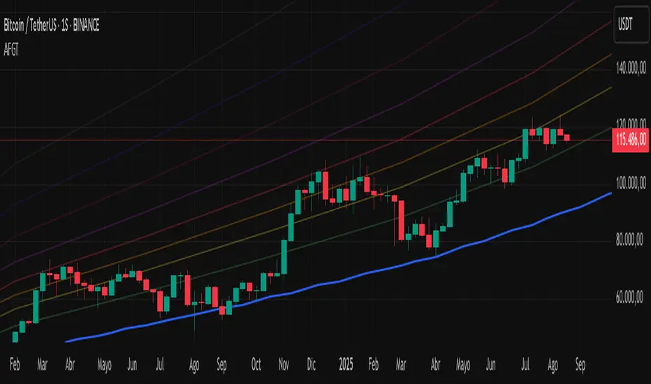
Auto-Fit Growth Trendline# **Theoretical Algorithmic Principles of the Auto-Fit Growth Trendline (AFGT)**
## **🎯 What Does This Algorithm Do?**
The Auto-Fit Growth Trendline is an advanced technical analysis system that **automates the identification of long-term growth trends** and **projects future price levels** based on historical cyclical patterns.
### **Primary Functionality:**
- **Automatically detects** the most significant lows in regular periods (monthly, quarterly, semi-annually, annually)
- **Constructs a dynamic trendline** that connects these historical lows
- **Projects the trend into the future** with high mathematical precision
- **Generates Fibonacci bands** that act as dynamic support and resistance levels
- **Automatically adapts** to different timeframes and market conditions
### **Strategic Purpose:**
The algorithm is designed to identify **fundamental value zones** where price has historically found support, enabling traders to:
- Identify optimal entry points for long positions
- Establish realistic price targets based on mathematical projections
- Recognize dynamic support and resistance levels
- Anticipate long-term price movements
---
## **🧮 Core Mathematical Foundations**
### **Adaptive Temporal Segmentation Theory**
The algorithm is based on **dynamic temporal partition theory**, where time is divided into mathematically coherent uniform intervals. It uses modular transformations to create bijective mappings between continuous timestamps and discrete periods, ensuring each temporal point belongs uniquely to a specific period.
**What does this achieve?** It allows the algorithm to automatically identify natural market cycles (annual, quarterly, etc.) without manual intervention, adapting to the inherent periodicity of each asset.
The temporal mapping function implements a **discrete affine transformation** that normalizes different frequencies (monthly, quarterly, semi-annual, annual) to a space of unique identifiers, enabling consistent cross-temporal comparative analysis.
---
## **📊 Local Extrema Detection Theory**
### **Multi-Point Retrospective Validation Principle**
Local minima detection is founded on **relative extrema theory with sliding window**. Instead of using a simple minimum finder, it implements a cross-validation system that examines the persistence of the extremum across multiple historical periods.
**What problem does this solve?** It eliminates false minima caused by temporal volatility, identifying only those points that represent true historical support levels with statistical significance.
This approach is based on the **statistical confirmation principle**, where a minimum is only considered valid if it maintains its extremum condition during a defined observation period, significantly reducing false positives caused by transitory volatility.
---
## **🔬 Robust Interpolation Theory with Outlier Control**
### **Contextual Adaptive Interpolation Model**
The mathematical core uses **piecewise linear interpolation with adaptive outlier correction**. The key innovation lies in implementing a **contextual anomaly detector** that identifies not only absolute extreme values, but relative deviations to the local context.
**Why is this important?** Financial markets contain extreme events (crashes, bubbles) that can distort projections. This system identifies and appropriately weights them without completely eliminating them, preserving directional information while attenuating distortions.
### **Implicit Bayesian Smoothing Algorithm**
When an outlier is detected (deviation >300% of local average), the system applies a **simplified Kalman filter** that combines the current observation with a local trend estimation, using a weight factor that preserves directional information while attenuating extreme fluctuations.
---
## **📈 Stabilized Extrapolation Theory**
### **Exponential Growth Model with Dampening**
Extrapolation is based on a **modified exponential growth model with progressive dampening**. It uses multiple historical points to calculate local growth ratios, implements statistical filtering to eliminate outliers, and applies a dampening factor that increases with extrapolation distance.
**What advantage does this offer?** Long-term projections in finance tend to be exponentially unrealistic. This system maintains short-to-medium term accuracy while converging toward realistic long-term projections, avoiding the typical "exponential explosions" of other methods.
### **Asymptotic Convergence Principle**
For long-term projections, the algorithm implements **controlled asymptotic convergence**, where growth ratios gradually converge toward pre-established limits, avoiding unrealistic exponential projections while preserving short-to-medium term accuracy.
---
## **🌟 Dynamic Fibonacci Projection Theory**
### **Continuous Proportional Scaling Model**
Fibonacci bands are constructed through **uniform proportional scaling** of the base curve, where each level represents a linear transformation of the main curve by a constant factor derived from the Fibonacci sequence.
**What is its practical utility?** It provides dynamic resistance and support levels that move with the trend, offering price targets and profit-taking points that automatically adapt to market evolution.
### **Topological Preservation Principle**
The system maintains the **topological properties** of the base curve in all Fibonacci projections, ensuring that spatial and temporal relationships are consistently preserved across all resistance/support levels.
---
## **⚡ Adaptive Computational Optimization**
### **Multi-Scale Resolution Theory**
It implements **automatic multi-resolution analysis** where data granularity is dynamically adjusted according to the analysis timeframe. It uses the **adaptive Nyquist principle** to optimize the signal-to-noise ratio according to the temporal observation scale.
**Why is this necessary?** Different timeframes require different levels of detail. A 1-minute chart needs more granularity than a monthly one. This system automatically optimizes resolution for each case.
### **Adaptive Density Algorithm**
Calculation point density is optimized through **adaptive sampling theory**, where calculation frequency is adjusted according to local trend curvature and analysis timeframe, balancing visual precision with computational efficiency.
---
## **🛡️ Robustness and Fault Tolerance**
### **Graceful Degradation Theory**
The system implements **multi-level graceful degradation**, where under error conditions or insufficient data, the algorithm progressively falls back to simpler but reliable methods, maintaining basic functionality under any condition.
**What does this guarantee?** That the indicator functions consistently even with incomplete data, new symbols with limited history, or extreme market conditions.
### **State Consistency Principle**
It uses **mathematical invariants** to guarantee that the algorithm's internal state remains consistent between executions, implementing consistency checks that validate data structure integrity in each iteration.
---
## **🔍 Key Theoretical Innovations**
### **A. Contextual vs. Absolute Outlier Detection**
It revolutionizes traditional outlier detection by considering not only the absolute magnitude of deviations, but their relative significance within the local context of the time series.
**Practical impact:** It distinguishes between legitimate market movements and technical anomalies, preserving important events like breakouts while filtering noise.
### **B. Extrapolation with Weighted Historical Memory**
It implements a memory system that weights different historical periods according to their relevance for current prediction, creating projections more adaptable to market regime changes.
**Competitive advantage:** It automatically adapts to fundamental changes in asset dynamics without requiring manual recalibration.
### **C. Automatic Multi-Timeframe Adaptation**
It develops an automatic temporal resolution selection system that optimizes signal extraction according to the intrinsic characteristics of the analysis timeframe.
**Result:** A single indicator that functions optimally from 1-minute to monthly charts without manual adjustments.
### **D. Intelligent Asymptotic Convergence**
It introduces the concept of controlled asymptotic convergence in financial extrapolations, where long-term projections converge toward realistic limits based on historical fundamentals.
**Added value:** Mathematically sound long-term projections that avoid the unrealistic extremes typical of other extrapolation methods.
---
## **📊 Complexity and Scalability Theory**
### **Optimized Linear Complexity Model**
The algorithm maintains **linear computational complexity** O(n) in the number of historical data points, guaranteeing scalability for extensive time series analysis without performance degradation.
### **Temporal Locality Principle**
It implements **temporal locality**, where the most expensive operations are concentrated in the most relevant temporal regions (recent periods and near projections), optimizing computational resource usage.
---
## **🎯 Convergence and Stability**
### **Probabilistic Convergence Theory**
The system guarantees **probabilistic convergence** toward the real underlying trend, where projection accuracy increases with the amount of available historical data, following **law of large numbers** principles.
**Practical implication:** The more history an asset has, the more accurate the algorithm's projections will be.
### **Guaranteed Numerical Stability**
It implements **intrinsic numerical stability** through the use of robust floating-point arithmetic and validations that prevent overflow, underflow, and numerical error propagation.
**Result:** Reliable operation even with extreme-priced assets (from satoshis to thousand-dollar stocks).
---
## **💼 Comprehensive Practical Application**
**The algorithm functions as a "financial GPS"** that:
1. **Identifies where we've been** (significant historical lows)
2. **Determines where we are** (current position relative to the trend)
3. **Projects where we're going** (future trend with specific price levels)
4. **Provides alternative routes** (Fibonacci bands as alternative targets)
This theoretical framework represents an innovative synthesis of time series analysis, approximation theory, and computational optimization, specifically designed for long-term financial trend analysis with robust and mathematically grounded projections.
Qullamaggie [Modified] | FractalystWhat's the purpose of this strategy?
The strategy aims to identify high-probability breakout setups in trending markets, inspired by Kristjan "Qullamaggie" Kullamägi’s approach.
It focuses on capturing explosive price moves after periods of consolidation, using technical criteria like moving averages, breakouts, trailing stop-loss and momentum confirmation.
Ideal for swing traders seeking to ride strong trends while managing risk.
----
How does the strategy work?
The strategy follows a systematic process to capture high-momentum breakouts:
Pre-Breakout Criteria:
Prior Price Surge: Identifies stocks that have rallied 30-100%+ in recent month(s), signaling strong underlying momentum (per Qullamaggie’s volatility expansion principles).
Consolidation Phase: Looks for a tightening price range (e.g., flag, pennant, or tight base), indicating a potential "coiling" before continuation.
Trend Confirmation: Uses moving averages (e.g., 20/50/200 EMA) to ensure the stock is trading above key averages on the daily chart, confirming an uptrend.
Price Break: Enters when price clears the consolidation high with conviction.
Risk Management:
Initial Stop Loss: Placed below the consolidation low or a recent swing point to limit downside.
Break-Even Adjustment: Moves stop loss to breakeven once the trade reaches 1.5x risk-to-reward (RR), securing a "free trade" while letting winners run.
Trailing Stop (Unique Edge):
Market Structure Trailing: Instead of trailing via moving averages, the stop is dynamically adjusted using structural invalidation level. This adapts to price action, allowing the trade to stay open during volatile retracements while locking in gains as new structure forms.
Why This Matters: Most strategies use rigid trailing stops (e.g., below the 10EMA), which often exit prematurely in choppy markets. By trailing based on structure, this strategy avoids "noise" and captures larger trends, directly boosting overall returns.
----
What markets or timeframes is this suited for?
This is a long-only strategy designed for trending markets, and it performs best in:
Markets: Stocks (especially high-growth, liquid equities), cryptocurrencies (major pairs with strong volatility), commodities (e.g., oil, gold), and futures (index/commodity futures).
Timeframes: Primarily daily charts for swing trades (1-30 day holds), though weekly charts can help confirm broader trends.
Key Advantage: The TradingView script allows instant backtesting with adjustable parameters
You can:
- Test historical performance across multiple markets to identify which assets align best with the strategy.
- Optimize settings (e.g., trailing stop sensitivity, moving averages etc.) to match a market’s volatility profile.
Build a diversified portfolio by filtering for markets that show consistent profitability in backtests.
For example, you might discover cryptos require tighter trailing stops due to volatility, while stocks thrive with wider structural stops. The script automates this analysis, letting you to trade confidently.
----
What indicators or tools does the strategy use?
The strategy combines customizable technical tools with strict anti-lookahead safeguards:
Core Indicators:
Moving Averages: Adjustable periods (e.g., 20/50/200 EMA or SMA) and timeframes (daily/weekly) to confirm trend alignment. Users can test combinations (e.g., 10EMA vs. 20EMA) to optimize for specific markets.
Breakout Parameters:
Consolidation Length: Adjustable window to define the "tightness" of the pre-breakout pattern.
Entry Models: Flexible entry logics (Breakouts and fractals)
Anti-Lookahead Design:
All calculations (e.g., moving averages, consolidation ranges, volume averages) use only closed/confirmed data available at the time of the signal.
----
How do I manage risk with this strategy?
The strategy prioritizes customizable risk controls to align with your trading style and account size:
User-Defined Risk Inputs:
Risk Per Trade: Set a % of Equity (e.g., 1-2%) to determine position size. The strategy auto-calculates shares/contracts to match your selected risk per trade.
Flexibility: Choose between fixed risk or equity-based scaling.
The script adjusts position sizing dynamically based on your selection.
Pyramiding Feature:
Customizable Entries: Adjust the number of pyramiding trades allowed (e.g., 1-3 additional positions) in the strategy settings. Each new entry is triggered only if the prior trade hits its 1.5x RR target and the trend remains intact.
Risk-Scaled Additions: New positions use profits from prior trades, compounding gains without increasing initial risk.
Risk-Free Trade Mechanic:
Once a trade reaches 1.5x RR, the stop loss is moved to breakeven, eliminating downside risk.
The strategy then opens a new position (if pyramiding is enabled) using a portion of the locked-in profit. This "snowballs" winners while keeping total capital exposure stable.
Impact on Net Profit & Drawdown:
Net Profit Boost: Pyramiding lets you ride multi-leg trends aggressively. For example, a 100% runner could generate 2-3x more profit vs. a single-entry approach.
Controlled Drawdowns: Since new positions are funded by profits (not initial capital), max drawdown stays anchored to your original risk per trade (e.g., 1-2% of account). Even if later entries fail, the breakeven stop on prior trades protects overall equity.
Why This Works: Most strategies either over-leverage (increasing drawdowns) or exit too early. By recycling profits into new positions only after securing risk-free capital, this approach mimics hedge fund "scaling in" tactics while staying retail-trader friendly.
----
How does the strategy identify market structure for its trailing stoploss?
The strategy identifies market structure by utilizing an efficient logic with for loops to pinpoint the first swing candle that features a pivot of 2. This marks the beginning of the break of structure, where the market's previous trend or pattern is considered invalidated or changed.
----
What are the underlying calculations?
The underlying calculations involve:
Identifying Swing Points: The strategy looks for swing highs (marked with blue Xs) and swing lows (marked with red Xs). A swing high is identified when a candle's high is higher than the highs of the candles before and after it. Conversely, a swing low is when a candle's low is lower than the lows of the candles before and after it.
Break of Structure (BOS):
Bullish BOS: This occurs when the price breaks above the swing high level of the previous structure, indicating a potential shift to a bullish trend.
Bearish BOS: This happens when the price breaks below the swing low level of the previous structure, signaling a potential shift to a bearish trend.
Structural Liquidity and Invalidation:
Structural Liquidity: After a break of structure, liquidity levels are updated to the first swing high in a bullish BOS or the first swing low in a bearish BOS.
Structural Invalidation: If the price moves back to the level of the first swing low before the bullish BOS or the first swing high before the bearish BOS, it invalidates the break of structure, suggesting a potential reversal or continuation of the previous trend.
This method provides users with a technical approach to filter market regimes, offering an advantage by minimizing the risk of overfitting to historical data, which is often a concern with traditional indicators like moving averages.
By focusing on identifying pivotal swing points and the subsequent breaks of structure, the strategy maintains a balance between sensitivity to market changes and robustness against historical data anomalies, ensuring a more adaptable and potentially more reliable market analysis tool.
----
What entry criteria are used in this script?
The script uses two entry models for trading decisions: BreakOut and Fractal.
Underlying Calculations:
Breakout: The script records the most recent swing high by storing it in a variable. When the price closes above this recorded level, and all other predefined conditions are satisfied, the script triggers a breakout entry. This approach is considered conservative because it waits for the price to confirm a breakout above the previous high before entering a trade. As shown in the image, as soon as the price closes above the new candle (first tick), the long entry gets taken. The stop-loss is initially set and then moved to break-even once the price moves in favor of the trade.
Fractal: This method involves identifying a swing low with a period of 2, which means it looks for a low point where the price is lower than the two candles before and after it. Once this pattern is detected, the script executes the trade. This is an aggressive approach since it doesn't wait for further price confirmation. In the image, this is represented by the 'Fractal 2' label where the script identifies and acts on the swing low pattern.
----
What type of stop-loss identification method are used in this strategy?
This strategy employs two types of stop-loss methods: Initial Stop-loss and Trailing Stop-Loss.
Underlying Calculations:
Initial Stop-loss:
ATR Based: The strategy uses the Average True Range (ATR) to set an initial stop-loss, which helps in accounting for market volatility without predicting price direction.
Calculation:
- First, the True Range (TR) is calculated for each period, which is the greatest of:
- Current Period High - Current Period Low
- Absolute Value of Current Period High - Previous Period Close
- Absolute Value of Current Period Low - Previous Period Close
- The ATR is then the moving average of these TR values over a specified period, typically 14 periods by default. This ATR value can be used to set the stop-loss at a distance from the entry price that reflects the current market volatility.
Swing Low Based:
For this method, the stop-loss is set based on the most recent swing low identified in the market structure analysis. This approach uses the lowest point of the recent price action as a reference for setting the stop-loss.
Trailing Stop-Loss:
The strategy uses structural liquidity and structural invalidation levels across multiple timeframes to adjust the stop-loss once the trade is profitable. This method involves:
Detecting Structural Liquidity: After a break of structure, the liquidity levels are updated to the first swing high in a bullish scenario or the first swing low in a bearish scenario. These levels serve as potential areas where the price might find support or resistance, allowing the stop-loss to trail the price movement.
Detecting Structural Invalidation: If the price returns to the level of the first swing low before a bullish break of structure or the first swing high before a bearish break of structure, it suggests the trend might be reversing or invalidating, prompting the adjustment of the stop-loss to lock in profits or minimize losses.
By using these methods, the strategy dynamically adjusts the initial stop-loss based on market volatility, helping to protect against adverse price movements while allowing for enough room for trades to develop. The ATR-based stop-loss adapts to the current market conditions by considering the volatility, ensuring that the stop-loss is not too tight during volatile periods, which could lead to premature exits, nor too loose during calm markets, which might result in larger losses. Similarly, the swing low based stop-loss provides a logical exit point if the market structure changes unfavorably.
Each market behaves differently across various timeframes, and it is essential to test different parameters and optimizations to find out which trailing stop-loss method gives you the desired results and performance. This involves backtesting the strategy with different settings for the ATR period, the distance from the swing low, and how the trailing stop-loss reacts to structural liquidity and invalidation levels.
Through this process, you can tailor the strategy to perform optimally in different market environments, ensuring that the stop-loss mechanism supports the trade's longevity while safeguarding against significant drawdowns.
----
What type of break-even method is used in this strategy? What are the underlying calculations?
Moves the initial stop-loss to the entry price when the price reaches a certain RR ratio.
Calculation:
Break-even level = Entry Price + (Initial Risk * RR Ratio)
----
What tables are available in this script?
- Summary: Provides a general overview, displaying key performance parameters such as Net Profit, Profit Factor, Max Drawdown, Average Trade, Closed Trades and more.
Total Commission: Displays the cumulative commissions incurred from all trades executed within the selected backtesting window. This value is derived by summing the commission fees for each trade on your chart.
Average Commission: Represents the average commission per trade, calculated by dividing the Total Commission by the total number of closed trades. This metric is crucial for assessing the impact of trading costs on overall profitability.
Avg Trade: The sum of money gained or lost by the average trade generated by a strategy. Calculated by dividing the Net Profit by the overall number of closed trades. An important value since it must be large enough to cover the commission and slippage costs of trading the strategy and still bring a profit.
MaxDD: Displays the largest drawdown of losses, i.e., the maximum possible loss that the strategy could have incurred among all of the trades it has made. This value is calculated separately for every bar that the strategy spends with an open position.
Profit Factor: The amount of money a trading strategy made for every unit of money it lost (in the selected currency). This value is calculated by dividing gross profits by gross losses.
Avg RR: This is calculated by dividing the average winning trade by the average losing trade. This field is not a very meaningful value by itself because it does not take into account the ratio of the number of winning vs losing trades, and strategies can have different approaches to profitability. A strategy may trade at every possibility in order to capture many small profits, yet have an average losing trade greater than the average winning trade. The higher this value is, the better, but it should be considered together with the percentage of winning trades and the net profit.
Winrate: The percentage of winning trades generated by a strategy. Calculated by dividing the number of winning trades by the total number of closed trades generated by a strategy. Percent profitable is not a very reliable measure by itself. A strategy could have many small winning trades, making the percent profitable high with a small average winning trade, or a few big winning trades accounting for a low percent profitable and a big average winning trade. Most mean-reversion successful strategies have a percent profitability of 40-80% but are profitable due to risk management control.
BE Trades: Number of break-even trades, excluding commission/slippage.
Losing Trades: The total number of losing trades generated by the strategy.
Winning Trades: The total number of winning trades generated by the strategy.
Total Trades: Total number of taken traders visible your charts.
Net Profit: The overall profit or loss (in the selected currency) achieved by the trading strategy in the test period. The value is the sum of all values from the Profit column (on the List of Trades tab), taking into account the sign.
- Monthly: Displays performance data on a month-by-month basis, allowing users to analyze performance trends over each month and year.
- Weekly: Displays performance data on a week-by-week basis, helping users to understand weekly performance variations.
- UI Table: A user-friendly table that allows users to view and save the selected strategy parameters from user inputs. This table enables easy access to key settings and configurations, providing a straightforward solution for saving strategy parameters by simply taking a screenshot with Alt + S or ⌥ + S.
User-input styles and customizations:
Please note that all background colors in the style are disabled by default to enhance visualization.
How to Use This Strategy to Create a Profitable Edge and Systems?
Choose Your Strategy mode:
- Decide whether you are creating an investing strategy or a trading strategy.
Select a Market:
- Choose a one-sided market such as stocks, indices, or cryptocurrencies.
Historical Data:
- Ensure the historical data covers at least 10 years of price action for robust backtesting.
Timeframe Selection:
- Choose the timeframe you are comfortable trading with. It is strongly recommended to use a timeframe above 15 minutes to minimize the impact of commissions/slippage on your profits.
Set Commission and Slippage:
- Properly set the commission and slippage in the strategy properties according to your broker/prop firm specifications.
Parameter Optimization:
- Use trial and error to test different parameters until you find the performance results you are looking for in the summary table or, preferably, through deep backtesting using the strategy tester.
Trade Count:
- Ensure the number of trades is 200 or more; the higher, the better for statistical significance.
Positive Average Trade:
- Make sure the average trade is above zero.
(An important value since it must be large enough to cover the commission and slippage costs of trading the strategy and still bring a profit.)
Performance Metrics:
- Look for a high profit factor, and net profit with minimum drawdown.
- Ideally, aim for a drawdown under 20-30%, depending on your risk tolerance.
Refinement and Optimization:
- Try out different markets and timeframes.
- Continue working on refining your edge using the available filters and components to further optimize your strategy.
What Makes This Strategy Unique?
This strategy combines flexibility, smart risk management, and momentum focus in a way that’s rare and practical:
1. Adapts to Any Market Rhythm
Works on daily, weekly, or intraday charts without code changes.
Uses two entry types: classic breakouts (like trending stocks) or fractal patterns (to avoid false starts).
2. Smarter Stop-Loss System
No rigid rules: Stops adjust based on price structure (e.g., new “higher lows”), not fixed percentages.
Avoids whipsaws: Tightens stops only when the trend strengthens, not in choppy markets.
3. Safe Profit-Boosting Pyramiding
Adds new positions only after prior trades are risk-free (stops moved above breakeven).
Scales up using locked-in profits, not new capital, to grow gains safely.
4. Built-In Momentum Check
Tracks 1/3/6-month price growth to spotlight stocks with strong, lasting momentum.
Terms and Conditions | Disclaimer
Our charting tools are provided for informational and educational purposes only and should not be construed as financial, investment, or trading advice. They are not intended to forecast market movements or offer specific recommendations. Users should understand that past performance does not guarantee future results and should not base financial decisions solely on historical data.
Built-in components, features, and functionalities of our charting tools are the intellectual property of @Fractalyst Unauthorized use, reproduction, or distribution of these proprietary elements is prohibited.
- By continuing to use our charting tools, the user acknowledges and accepts the Terms and Conditions outlined in this legal disclaimer and agrees to respect our intellectual property rights and comply with all applicable laws and regulations.

Dollar Cost Averaging (DCA) | FractalystWhat's the purpose of this strategy?
The purpose of dollar cost averaging (DCA) is to grow investments over time using a disciplined, methodical approach used by many top institutions like MicroStrategy and other institutions.
Here's how it functions:
Dollar Cost Averaging (DCA): This technique involves investing a set amount of money regularly, regardless of market conditions. It helps to mitigate the risk of investing a large sum at a peak price by spreading out your investment, thus potentially lowering your average cost per share over time.
Regular Contributions: By adding money to your investments on a pre-determined frequency and dollar amount defined by the user, you take advantage of compounding. The script will remind you to contribute based on your chosen schedule, which can be weekly, bi-weekly, monthly, quarterly, or yearly. This systematic approach ensures that your returns can earn their own returns, much like interest on savings but potentially at a higher rate.
Technical Analysis: The strategy employs a market trend ratio to gauge market sentiment. It calculates the ratio of bullish vs bearish breakouts across various timeframes, assigning this ratio a percentage-based score to determine the directional bias. Once this score exceeds a user-selected percentage, the strategy looks to take buy entries, signaling a favorable time for investment based on current market trends.
Fundamental Analysis: This aspect looks at the health of the economy and companies within it to determine bullish market conditions. Specifically, we consider:
Specifically, it considers:
Interest Rate: High interest rates can affect borrowing costs, potentially slowing down economic growth or making stocks less attractive compared to fixed income.
Inflation Rate: Inflation erodes purchasing power, but moderate inflation can be a sign of a healthy economy. We look for investments that might benefit from or withstand inflation.
GDP Rate: GDP growth indicates the overall health of the economy; we aim to invest in sectors poised to grow with the economy.
Unemployment Rate: Lower unemployment typically signals consumer confidence and spending power, which can boost certain sectors.
By integrating these elements, the strategy aims to:
Reduce Investment Volatility: By spreading out your investments, you're less impacted by short-term market swings.
Enhance Growth Potential: Using both technical and fundamental filters helps in choosing investments that are more likely to appreciate over time.
Manage Risk: The strategy aims to balance the risk of market timing by investing consistently and choosing assets wisely based on both economic data and market conditions.
----
What are Regular Contributions in this strategy?
Regular Contributions involve adding money to your investments on a pre-determined frequency and dollar amount defined by the user. The script will remind you to contribute based on your chosen schedule, which can be weekly, bi-weekly, monthly, quarterly, or yearly. This systematic approach ensures that your returns can earn their own returns, much like interest on savings but potentially at a higher rate.
----
How do regular contributions enhance compounding and reduce timing risk?
Enhances Compounding: Regular contributions leverage the power of compounding, where returns on investments can generate their own returns, potentially leading to exponential growth over time.
Reduces Timing Risk: By investing regularly, the strategy minimizes the risk associated with trying to time the market, spreading out the investment cost over time and potentially reducing the impact of volatility.
Automated Reminders: The script reminds users to make contributions based on their chosen schedule, ensuring consistency and discipline in investment practices, which is crucial for long-term success.
----
How does the strategy integrate technical and fundamental analysis for investors?
A: The strategy combines technical and fundamental analysis in the following manner:
Technical Analysis: It uses a market trend ratio to determine the directional bias by calculating the ratio of bullish vs bearish breakouts. Once this ratio exceeds a user-selected percentage threshold, the strategy signals to take buy entries, optimizing the timing within the given timeframe(s).
Fundamental Analysis: This aspect assesses the broader economic environment to identify sectors or assets that are likely to benefit from current economic conditions. By understanding these fundamentals, the strategy ensures investments are made in assets with strong growth potential.
This integration allows the strategy to select investments that are both technically favorable for entry and fundamentally sound, providing a comprehensive approach to investment decisions in the crypto, stock, and commodities markets.
----
How does the strategy identify market structure? What are the underlying calculations?
Q: How does the strategy identify market structure?
A: The strategy identifies market structure by utilizing an efficient logic with for loops to pinpoint the first swing candle that features a pivot of 2. This marks the beginning of the break of structure, where the market's previous trend or pattern is considered invalidated or changed.
What are the underlying calculations for identifying market structure?
A: The underlying calculations involve:
Identifying Swing Points: The strategy looks for swing highs (marked with blue Xs) and swing lows (marked with red Xs). A swing high is identified when a candle's high is higher than the highs of the candles before and after it. Conversely, a swing low is when a candle's low is lower than the lows of the candles before and after it.
Break of Structure (BOS):
Bullish BOS: This occurs when the price breaks above the swing high level of the previous structure, indicating a potential shift to a bullish trend.
Bearish BOS: This happens when the price breaks below the swing low level of the previous structure, signaling a potential shift to a bearish trend.
Structural Liquidity and Invalidation:
Structural Liquidity: After a break of structure, liquidity levels are updated to the first swing high in a bullish BOS or the first swing low in a bearish BOS.
Structural Invalidation: If the price moves back to the level of the first swing low before the bullish BOS or the first swing high before the bearish BOS, it invalidates the break of structure, suggesting a potential reversal or continuation of the previous trend.
This method provides users with a technical approach to filter market regimes, offering an advantage by minimizing the risk of overfitting to historical data, which is often a concern with traditional indicators like moving averages.
By focusing on identifying pivotal swing points and the subsequent breaks of structure, the strategy maintains a balance between sensitivity to market changes and robustness against historical data anomalies, ensuring a more adaptable and potentially more reliable market analysis tool.
What entry criteria are used in this script?
The script uses two entry models for trading decisions: BreakOut and Fractal.
Underlying Calculations:
Breakout: The script records the most recent swing high by storing it in a variable. When the price closes above this recorded level, and all other predefined conditions are satisfied, the script triggers a breakout entry. This approach is considered conservative because it waits for the price to confirm a breakout above the previous high before entering a trade. As shown in the image, as soon as the price closes above the new candle (first tick), the long entry gets taken. The stop-loss is initially set and then moved to break-even once the price moves in favor of the trade.
Fractal: This method involves identifying a swing low with a period of 2, which means it looks for a low point where the price is lower than the two candles before and after it. Once this pattern is detected, the script executes the trade. This is an aggressive approach since it doesn't wait for further price confirmation. In the image, this is represented by the 'Fractal 2' label where the script identifies and acts on the swing low pattern.
----
How does the script calculate trend score? What are the underlying calculations?
Market Trend Ratio: The script calculates the ratio of bullish to bearish breakouts. This involves:
Counting Bullish Breakouts: A bullish breakout is counted when the price breaks above a recent swing high (as identified in the strategy's market structure analysis).
Counting Bearish Breakouts: A bearish breakout is counted when the price breaks below a recent swing low.
Percentage-Based Score: This ratio is then converted into a percentage-based score:
For example, if there are 10 bullish breakouts and 5 bearish breakouts in a given timeframe, the ratio would be 10:5 or 2:1. This could be translated into a score where 66.67% (10/(10+5) * 100) represents the bullish trend strength.
The score might be calculated as (Number of Bullish Breakouts / Total Breakouts) * 100.
User-Defined Threshold: The strategy uses this score to determine when to take buy entries. If the trend score exceeds a user-defined percentage threshold, it indicates a strong enough bullish trend to justify a buy entry. For instance, if the user sets the threshold at 60%, the script would look for a buy entry when the trend score is above this level.
Timeframe Consideration: The calculations are performed across the timeframes specified by the user, ensuring the trend score reflects the market's behavior over different periods, which could be daily, weekly, or any other relevant timeframe.
This method provides a quantitative measure of market trend strength, helping to make informed decisions based on the balance between bullish and bearish market movements.
What type of stop-loss identification method are used in this strategy?
This strategy employs two types of stop-loss methods: Initial Stop-loss and Trailing Stop-Loss.
Underlying Calculations:
Initial Stop-loss:
ATR Based: The strategy uses the Average True Range (ATR) to set an initial stop-loss, which helps in accounting for market volatility without predicting price direction.
Calculation:
- First, the True Range (TR) is calculated for each period, which is the greatest of:
- Current Period High - Current Period Low
- Absolute Value of Current Period High - Previous Period Close
- Absolute Value of Current Period Low - Previous Period Close
- The ATR is then the moving average of these TR values over a specified period, typically 14 periods by default. This ATR value can be used to set the stop-loss at a distance from the entry price that reflects the current market volatility.
Swing Low Based:
For this method, the stop-loss is set based on the most recent swing low identified in the market structure analysis. This approach uses the lowest point of the recent price action as a reference for setting the stop-loss.
Trailing Stop-Loss:
The strategy uses structural liquidity and structural invalidation levels across multiple timeframes to adjust the stop-loss once the trade is profitable. This method involves:
Detecting Structural Liquidity: After a break of structure, the liquidity levels are updated to the first swing high in a bullish scenario or the first swing low in a bearish scenario. These levels serve as potential areas where the price might find support or resistance, allowing the stop-loss to trail the price movement.
Detecting Structural Invalidation: If the price returns to the level of the first swing low before a bullish break of structure or the first swing high before a bearish break of structure, it suggests the trend might be reversing or invalidating, prompting the adjustment of the stop-loss to lock in profits or minimize losses.
By using these methods, the strategy dynamically adjusts the initial stop-loss based on market volatility, helping to protect against adverse price movements while allowing for enough room for trades to develop. The ATR-based stop-loss adapts to the current market conditions by considering the volatility, ensuring that the stop-loss is not too tight during volatile periods, which could lead to premature exits, nor too loose during calm markets, which might result in larger losses. Similarly, the swing low based stop-loss provides a logical exit point if the market structure changes unfavorably.
Each market behaves differently across various timeframes, and it is essential to test different parameters and optimizations to find out which trailing stop-loss method gives you the desired results and performance. This involves backtesting the strategy with different settings for the ATR period, the distance from the swing low, and how the trailing stop-loss reacts to structural liquidity and invalidation levels.
Through this process, you can tailor the strategy to perform optimally in different market environments, ensuring that the stop-loss mechanism supports the trade's longevity while safeguarding against significant drawdowns.
What type of break-even and take profit identification methods are used in this strategy? What are the underlying calculations?
For Break-Even:
Percentage (%) Based:
Moves the initial stop-loss to the entry price when the price reaches a certain percentage above the entry.
Calculation:
Break-even level = Entry Price * (1 + Percentage / 100)
Example:
If the entry price is $100 and the break-even percentage is 5%, the break-even level is $100 * 1.05 = $105.
Risk-to-Reward (RR) Based:
Moves the initial stop-loss to the entry price when the price reaches a certain RR ratio.
Calculation:
Break-even level = Entry Price + (Initial Risk * RR Ratio)
For TP
- You can choose to set a take profit level at which your position gets fully closed.
- Similar to break-even, you can select either a percentage (%) or risk-to-reward (RR) based take profit level, allowing you to set your TP1 level as a percentage amount above the entry price or based on RR.
What's the day filter Filter, what does it do?
The day filter allows users to customize the session time and choose the specific days they want to include in the strategy session. This helps traders tailor their strategies to particular trading sessions or days of the week when they believe the market conditions are more favorable for their trading style.
Customize Session Time:
Users can define the start and end times for the trading session.
This allows the strategy to only consider trades within the specified time window, focusing on periods of higher market activity or preferred trading hours.
Select Days:
Users can select which days of the week to include in the strategy.
This feature is useful for excluding days with historically lower volatility or unfavorable trading conditions (e.g., Mondays or Fridays).
Benefits:
Focus on Optimal Trading Periods:
By customizing session times and days, traders can focus on periods when the market is more likely to present profitable opportunities.
Avoid Unfavorable Conditions:
Excluding specific days or times can help avoid trading during periods of low liquidity or high unpredictability, such as major news events or holidays.
What tables are available in this script?
- Summary: Provides a general overview, displaying key performance parameters such as Net Profit, Profit Factor, Max Drawdown, Average Trade, Closed Trades and more.
Total Commission: Displays the cumulative commissions incurred from all trades executed within the selected backtesting window. This value is derived by summing the commission fees for each trade on your chart.
Average Commission: Represents the average commission per trade, calculated by dividing the Total Commission by the total number of closed trades. This metric is crucial for assessing the impact of trading costs on overall profitability.
Avg Trade: The sum of money gained or lost by the average trade generated by a strategy. Calculated by dividing the Net Profit by the overall number of closed trades. An important value since it must be large enough to cover the commission and slippage costs of trading the strategy and still bring a profit.
MaxDD: Displays the largest drawdown of losses, i.e., the maximum possible loss that the strategy could have incurred among all of the trades it has made. This value is calculated separately for every bar that the strategy spends with an open position.
Profit Factor: The amount of money a trading strategy made for every unit of money it lost (in the selected currency). This value is calculated by dividing gross profits by gross losses.
Avg RR: This is calculated by dividing the average winning trade by the average losing trade. This field is not a very meaningful value by itself because it does not take into account the ratio of the number of winning vs losing trades, and strategies can have different approaches to profitability. A strategy may trade at every possibility in order to capture many small profits, yet have an average losing trade greater than the average winning trade. The higher this value is, the better, but it should be considered together with the percentage of winning trades and the net profit.
Winrate: The percentage of winning trades generated by a strategy. Calculated by dividing the number of winning trades by the total number of closed trades generated by a strategy. Percent profitable is not a very reliable measure by itself. A strategy could have many small winning trades, making the percent profitable high with a small average winning trade, or a few big winning trades accounting for a low percent profitable and a big average winning trade. Most mean-reversion successful strategies have a percent profitability of 40-80% but are profitable due to risk management control.
BE Trades: Number of break-even trades, excluding commission/slippage.
Losing Trades: The total number of losing trades generated by the strategy.
Winning Trades: The total number of winning trades generated by the strategy.
Total Trades: Total number of taken traders visible your charts.
Net Profit: The overall profit or loss (in the selected currency) achieved by the trading strategy in the test period. The value is the sum of all values from the Profit column (on the List of Trades tab), taking into account the sign.
- Monthly: Displays performance data on a month-by-month basis, allowing users to analyze performance trends over each month and year.
- Weekly: Displays performance data on a week-by-week basis, helping users to understand weekly performance variations.
- UI Table: A user-friendly table that allows users to view and save the selected strategy parameters from user inputs. This table enables easy access to key settings and configurations, providing a straightforward solution for saving strategy parameters by simply taking a screenshot with Alt + S or ⌥ + S.
User-input styles and customizations:
Please note that all background colors in the style are disabled by default to enhance visualization.
How to Use This Strategy to Create a Profitable Edge and Systems?
Choose Your Strategy mode:
- Decide whether you are creating an investing strategy or a trading strategy.
Select a Market:
- Choose a one-sided market such as stocks, indices, or cryptocurrencies.
Historical Data:
- Ensure the historical data covers at least 10 years of price action for robust backtesting.
Timeframe Selection:
- Choose the timeframe you are comfortable trading with. It is strongly recommended to use a timeframe above 15 minutes to minimize the impact of commissions/slippage on your profits.
Set Commission and Slippage:
- Properly set the commission and slippage in the strategy properties according to your broker/prop firm specifications.
Parameter Optimization:
- Use trial and error to test different parameters until you find the performance results you are looking for in the summary table or, preferably, through deep backtesting using the strategy tester.
Trade Count:
- Ensure the number of trades is 200 or more; the higher, the better for statistical significance.
Positive Average Trade:
- Make sure the average trade is above zero.
(An important value since it must be large enough to cover the commission and slippage costs of trading the strategy and still bring a profit.)
Performance Metrics:
- Look for a high profit factor, and net profit with minimum drawdown.
- Ideally, aim for a drawdown under 20-30%, depending on your risk tolerance.
Refinement and Optimization:
- Try out different markets and timeframes.
- Continue working on refining your edge using the available filters and components to further optimize your strategy.
What makes this strategy original?
Incorporation of Fundamental Analysis:
This strategy integrates fundamental analysis by considering key economic indicators such as interest rates, inflation, GDP growth, and unemployment rates. These fundamentals help in assessing the broader economic health, which in turn influences sector performance and market trends. By understanding these economic conditions, the strategy can identify sectors or assets that are likely to thrive, ensuring investments are made in environments conducive to growth. This approach allows for a more informed investment decision, aligning technical entries with fundamentally strong market conditions, thus potentially enhancing the strategy's effectiveness over time.
Technical Analysis Without Classical Methods:
The strategy's technical analysis diverges from traditional methods like moving averages by focusing on market structure through a trend score system.
Instead of using lagging indicators, it employs a real-time analysis of market trends by calculating the ratio of bullish to bearish breakouts. This provides several benefits:
Immediate Market Sentiment: The trend score system reacts more dynamically to current market conditions, offering insights into the market's immediate sentiment rather than historical trends, which can often lag behind real-time changes.
Reduced Overfitting: By not relying on moving averages or similar classical indicators, the strategy avoids the common pitfall of overfitting to historical data, which can lead to poor performance in new market conditions. The trend score provides a fresh perspective on market direction, potentially leading to more robust trading signals.
Clear Entry Signals: With the trend score, entry decisions are based on a clear percentage threshold, making the strategy's decision-making process straightforward and less subjective than interpreting moving average crossovers or similar signals.
Regular Contributions and Reminders:
The strategy encourages regular investments through a system of predefined frequency and amount, which could be weekly, bi-weekly, monthly, quarterly, or yearly. This systematic approach:
Enhances Compounding: Regular contributions leverage the power of compounding, where returns on investments can generate their own returns, potentially leading to exponential growth over time.
Reduces Timing Risk: By investing regularly, the strategy minimizes the risk associated with trying to time the market, spreading out the investment cost over time and potentially reducing the impact of volatility.
Automated Reminders: The script reminds users to make contributions based on their chosen schedule, ensuring consistency and discipline in investment practices, which is crucial for long-term success.
Long-Term Wealth Building:
Focused on long-term wealth accumulation, this strategy:
Promotes Patience and Discipline: By emphasizing regular contributions and a disciplined approach to both entry and risk management, it aligns with the principles of long-term investing, discouraging impulsive decisions based on short-term market fluctuations.
Diversification Across Asset Classes: Operating across crypto, stocks, and commodities, the strategy provides diversification, which is a key component of long-term wealth building, reducing risk through varied exposure.
Growth Over Time: The strategy's design to work with the market's natural growth cycles, supported by fundamental analysis, aims for sustainable growth rather than quick profits, aligning with the goals of investors looking to build wealth over decades.
This comprehensive approach, combining fundamental insights, innovative technical analysis, disciplined investment habits, and a focus on long-term growth, offers a unique and potentially effective pathway for investors seeking to build wealth steadily over time.
Terms and Conditions | Disclaimer
Our charting tools are provided for informational and educational purposes only and should not be construed as financial, investment, or trading advice. They are not intended to forecast market movements or offer specific recommendations. Users should understand that past performance does not guarantee future results and should not base financial decisions solely on historical data.
Built-in components, features, and functionalities of our charting tools are the intellectual property of @Fractalyst Unauthorized use, reproduction, or distribution of these proprietary elements is prohibited.
- By continuing to use our charting tools, the user acknowledges and accepts the Terms and Conditions outlined in this legal disclaimer and agrees to respect our intellectual property rights and comply with all applicable laws and regulations.

AlgoBuilder [Trend-Following] | FractalystWhat's the strategy's purpose and functionality?
This strategy is designed for both traders and investors looking to rely on and trade based on historical and backtested data using automation. The main goal is to build profitable trend-following strategies that outperform the underlying asset in terms of returns while minimizing drawdown. For example, as for a benchmark, if the S&P 500 (SPX) has achieved an estimated 10% annual return with a maximum drawdown of -57% over the past 20 years, using this strategy with different entry and exit techniques, users can potentially seek ways to achieve a higher Compound Annual Growth Rate (CAGR) while maintaining a lower maximum drawdown.
Although the strategy can be applied to all markets and timeframes, it is most effective on stocks, indices, future markets, cryptocurrencies, and commodities and JPY currency pairs given their trending behaviors.
In trending market conditions, the strategy employs a combination of moving averages and diverse entry models to identify and capitalize on upward market movements. It integrates market structure-based trailing stop-loss mechanisms across different timeframes and provides exit techniques, including percentage-based and risk-reward (RR) based take profit levels.
Additionally, the strategy has also a feature that includes a built-in probability and sentiment function for traders who want to implement probabilities and market sentiment right into their trading strategies.
Performance summary, weekly, and monthly tables enable quick visualization of performance metrics like net profit, maximum drawdown, compound annual growth rate (CAGR), profit factor, average trade, average risk-reward ratio (RR), and more. This aids optimization to meet specific goals and risk tolerance levels effectively.
-----
How does the strategy perform for both investors and traders?
The strategy has two main modes, tailored for different market participants: Traders and Investors.
Trading:
1. Trading (1x):
- Designed for traders looking to capitalize on bullish trending markets.
- Utilizes a percentage risk per trade to manage risk and optimize returns.
- Suitable for active trading with a focus on trend-following and risk management.
- (1x) This mode ensures no stacking of positions, allowing for only one running position or trade at a time.
◓: Mode | %: Risk percentage per trade
2. Trading (2x):
Similar to the 1x mode but allows for two pyramiding entries.
This approach enables traders to increase their position size as the trade moves in their favor, potentially enhancing profits during strong bullish trends.
◓: Mode | %: Risk percentage per trade
3. Investing:
- Geared towards investors who aim to capitalize on bullish trending markets without using leverage while mitigating the asset's maximum drawdown.
- Utilizes 100% of the equity to buy, hold, and manage the asset.
- Focuses on long-term growth and capital appreciation by fully investing in the asset during bullish conditions.
- ◓: Mode | %: Risk not applied (In investing mode, the strategy uses 100% of equity to buy the asset)
-----
What's the purpose of using moving averages in this strategy? What are the underlying calculations?
Using moving averages is a widely-used technique to trade with the trend.
The main purpose of using moving averages in this strategy is to filter out bearish price action and to only take trades when the price is trading ABOVE specified moving averages.
The script uses different types of moving averages with user-adjustable timeframes and periods/lengths, allowing traders to try out different variations to maximize strategy performance and minimize drawdowns.
By applying these calculations, the strategy effectively identifies bullish trends and avoids market conditions that are not conducive to profitable trades.
The MA filter allows traders to choose whether they want a specific moving average above or below another one as their entry condition.
This comparison filter can be turned on (>/<) or off.
For example, you can set the filter so that MA#1 > MA#2, meaning the first moving average must be above the second one before the script looks for entry conditions. This adds an extra layer of trend confirmation, ensuring that trades are only taken in more favorable market conditions.
MA #1: Fast MA | MA #2: Medium MA | MA #3: Slow MA
⍺: MA Period | Σ: MA Timeframe
-----
What entry modes are used in this strategy? What are the underlying calculations?
The strategy by default uses two different techniques for the entry criteria with user-adjustable left and right bars: Breakout and Fractal.
1. Breakout Entries :
- The strategy looks for pivot high points with a default period of 3.
- It stores the most recent high level in a variable.
- When the price crosses above this most recent level, the strategy checks if all conditions are met and the bar is closed before taking the buy entry.
◧: Pivot high left bars period | ◨: Pivot high right bars period
2. Fractal Entries :
- The strategy looks for pivot low points with a default period of 3.
- When a pivot low is detected, the strategy checks if all conditions are met and the bar is closed before taking the buy entry.
◧: Pivot low left bars period | ◨: Pivot low right bars period
By utilizing these entry modes, the strategy aims to capitalize on bullish price movements while ensuring that the necessary conditions are met to validate the entry points.
-----
What type of stop-loss identification method are used in this strategy? What are the underlying calculations?
Initial Stop-Loss:
1. ATR Based:
The Average True Range (ATR) is a method used in technical analysis to measure volatility. It is not used to indicate the direction of price but to measure volatility, especially volatility caused by price gaps or limit moves.
Calculation:
- To calculate the ATR, the True Range (TR) first needs to be identified. The TR takes into account the most current period high/low range as well as the previous period close.
The True Range is the largest of the following:
- Current Period High minus Current Period Low
- Absolute Value of Current Period High minus Previous Period Close
- Absolute Value of Current Period Low minus Previous Period Close
- The ATR is then calculated as the moving average of the TR over a specified period. (The default period is 14).
Example - ATR (14) * 1.5
⍺: ATR period | Σ: ATR Multiplier
2. ADR Based:
The Average Day Range (ADR) is an indicator that measures the volatility of an asset by showing the average movement of the price between the high and the low over the last several days.
Calculation:
- To calculate the ADR for a particular day:
- Calculate the average of the high prices over a specified number of days.
- Calculate the average of the low prices over the same number of days.
- Find the difference between these average values.
- The default period for calculating the ADR is 14 days. A shorter period may introduce more noise, while a longer period may be slower to react to new market movements.
Example - ADR (14) * 1.5
⍺: ADR period | Σ: ADR Multiplier
Application in Strategy:
- The strategy calculates the current bar's ADR/ATR with a user-defined period.
- It then multiplies the ADR/ATR by a user-defined multiplier to determine the initial stop-loss level.
By using these methods, the strategy dynamically adjusts the initial stop-loss based on market volatility, helping to protect against adverse price movements while allowing for enough room for trades to develop.
Trailing Stop-Loss:
One of the key elements of this strategy is its ability to detec buyside and sellside liquidity levels across multiple timeframes to trail the stop-loss once the trade is in running profits.
By utilizing this approach, the strategy allows enough room for price to run.
There are two built-in trailing stop-loss (SL) options you can choose from while in a trade:
1. External Trailing Stop-Loss:
- Uses sell-side liquidity to trail your stop-loss, allowing price to consolidate before continuation. This method is less aggressive and provides more room for price fluctuations.
Example - External - Wick below the trailing SL - 12H trailing timeframe
⍺: Exit type | Σ: Trailing stop-loss timeframe
2. Internal Trailing Stop-Loss:
- Uses the most recent swing low with a period of 2 to trail your stop-loss. This method is more aggressive compared to the external trailing stop-loss, as it tightens the stop-loss closer to the current price action.
Example - Internal - Close below the trailing SL - 6H trailing timeframe
⍺: Exit type | Σ: Trailing stop-loss timeframe
Each market behaves differently across various timeframes, and it is essential to test different parameters and optimizations to find out which trailing stop-loss method gives you the desired results and performance.
-----
What type of break-even and take profit identification methods are used in this strategy? What are the underlying calculations?
For Break-Even:
- You can choose to set a break-even level at which your initial stop-loss moves to the entry price as soon as it hits, and your trailing stop-loss gets activated (if enabled).
- You can select either a percentage (%) or risk-to-reward (RR) based break-even, allowing you to set your break-even level as a percentage amount above the entry price or based on RR.
For TP1 (Take Profit 1):
- You can choose to set a take profit level at which your position gets fully closed or 50% if the TP2 boolean is enabled.
- Similar to break-even, you can select either a percentage (%) or risk-to-reward (RR) based take profit level, allowing you to set your TP1 level as a percentage amount above the entry price or based on RR.
For TP2 (Take Profit 2):
- You can choose to set a take profit level at which your position gets fully closed.
- As with break-even and TP1, you can select either a percentage (%) or risk-to-reward (RR) based take profit level, allowing you to set your TP2 level as a percentage amount above the entry price or based on RR.
The underlying calculations involve determining the price levels at which these actions are triggered. For break-even, it moves the initial stop-loss to the entry price and activate the trailing stop-loss once the break-even level is reached.
For TP1 and TP2, it's specifying the price levels at which the position is partially or fully closed based on the chosen method (percentage or RR) above the entry price.
These calculations are crucial for managing risk and optimizing profitability in the strategy.
⍺: BE/TP type (%/RR) | Σ: how many RR/% above the current price
-----
What's the ADR filter? What does it do? What are the underlying calculations?
The Average Day Range (ADR) measures the volatility of an asset by showing the average movement of the price between the high and the low over the last several days.
The period of the ADR filter used in this strategy is tied to the same period you've used for your initial stop-loss.
Users can define the minimum ADR they want to be met before the script looks for entry conditions.
ADR Bias Filter:
- Compares the current bar ADR with the ADR (Defined by user):
- If the current ADR is higher, it indicates that volatility has increased compared to ADR (DbU).(⬆)
- If the current ADR is lower, it indicates that volatility has decreased compared to ADR (DbU).(⬇)
Calculations:
1. Calculate ADR:
- Average the high prices over the specified period.
- Average the low prices over the same period.
- Find the difference between these average values in %.
2. Current ADR vs. ADR (DbU):
- Calculate the ADR for the current bar.
- Calculate the ADR (DbU).
- Compare the two values to determine if volatility has increased or decreased.
By using the ADR filter, the strategy ensures that trades are only taken in favorable market conditions where volatility meets the user's defined threshold, thus optimizing entry conditions and potentially improving the overall performance of the strategy.
>: Minimum required ADR for entry | %: Current ADR comparison to ADR of 14 days ago.
-----
What's the probability filter? What are the underlying calculations?
The probability filter is designed to enhance trade entries by using buyside liquidity and probability analysis to filter out unfavorable conditions.
This filter helps in identifying optimal entry points where the likelihood of a profitable trade is higher.
Calculations:
1. Understanding Swing highs and Swing Lows
Swing High: A Swing High is formed when there is a high with 2 lower highs to the left and right.
Swing Low: A Swing Low is formed when there is a low with 2 higher lows to the left and right.
2. Understanding the purpose and the underlying calculations behind Buyside, Sellside and Equilibrium levels.
3. Understanding probability calculations
1. Upon the formation of a new range, the script waits for the price to reach and tap into equilibrium or the 50% level. Status: "⏸" - Inactive
2. Once equilibrium is tapped into, the equilibrium status becomes activated and it waits for either liquidity side to be hit. Status: "▶" - Active
3. If the buyside liquidity is hit, the script adds to the count of successful buyside liquidity occurrences. Similarly, if the sellside is tapped, it records successful sellside liquidity occurrences.
5. Finally, the number of successful occurrences for each side is divided by the overall count individually to calculate the range probabilities.
Note: The calculations are performed independently for each directional range. A range is considered bearish if the previous breakout was through a sellside liquidity. Conversely, a range is considered bullish if the most recent breakout was through a buyside liquidity.
Example - BSL > 50%
-----
What's the sentiment Filter? What are the underlying calculations?
Sentiment filter aims to calculate the percentage level of bullish or bearish fluctuations within equally divided price sections, in the latest price range.
Calculations:
This filter calculates the current sentiment by identifying the highest swing high and the lowest swing low, then evenly dividing the distance between them into percentage amounts. If the price is above the 50% mark, it indicates bullishness, whereas if it's below 50%, it suggests bearishness.
Sentiment Bias Identification:
Bullish Bias: The current price is trading above the 50% daily range.
Bearish Bias: The current price is trading below the 50% daily range.
Example - Sentiment Enabled | Bullish degree above 50% | Bullish sentimental bias
>: Minimum required sentiment for entry | %: Current sentimental degree in a (Bullish/Bearish) sentimental bias
-----
What's the range length Filter? What are the underlying calculations?
The range length filter identifies the price distance between buyside and sellside liquidity levels in percentage terms. When enabled, the script only looks for entries when the minimum range length is met. This helps ensure that trades are taken in markets with sufficient price movement.
Calculations:
Range Length (%) = ( ( Buyside Level − Sellside Level ) / Current Price ) ×100
Range Bias Identification:
Bullish Bias: The current range price has broken above the previous external swing high.
Bearish Bias: The current range price has broken below the previous external swing low.
Example - Range length filter is enabled | Range must be above 5% | Price must be in a bearish range
>: Minimum required range length for entry | %: Current range length percentage in a (Bullish/Bearish) range
-----
What's the day filter Filter, what does it do?
The day filter allows users to customize the session time and choose the specific days they want to include in the strategy session. This helps traders tailor their strategies to particular trading sessions or days of the week when they believe the market conditions are more favorable for their trading style.
Customize Session Time:
Users can define the start and end times for the trading session.
This allows the strategy to only consider trades within the specified time window, focusing on periods of higher market activity or preferred trading hours.
Select Days:
Users can select which days of the week to include in the strategy.
This feature is useful for excluding days with historically lower volatility or unfavorable trading conditions (e.g., Mondays or Fridays).
Benefits:
Focus on Optimal Trading Periods:
By customizing session times and days, traders can focus on periods when the market is more likely to present profitable opportunities.
Avoid Unfavorable Conditions:
Excluding specific days or times can help avoid trading during periods of low liquidity or high unpredictability, such as major news events or holidays.
Increased Flexibility: The filter provides increased flexibility, allowing traders to adapt the strategy to their specific needs and preferences.
Example - Day filter | Session Filter
θ: Session time | Exchange time-zone
-----
What tables are available in this script?
Table Type:
- Summary: Provides a general overview, displaying key performance parameters such as Net Profit, Profit Factor, Max Drawdown, Average Trade, Closed Trades, Compound Annual Growth Rate (CAGR), MAR and more.
CAGR: It calculates the 'Compound Annual Growth Rate' first and last taken trades on your chart. The CAGR is a notional, annualized growth rate that assumes all profits are reinvested. It only takes into account the prices of the two end points — not drawdowns, so it does not calculate risk. It can be used as a yardstick to compare the performance of two strategies. Since it annualizes values, it requires a minimum 4H timeframe to display the CAGR value. annualizing returns over smaller periods of times doesn't produce very meaningful figures.
MAR: Measure of return adjusted for risk: CAGR divided by Max Drawdown. Indicates how comfortable the system might be to trade. Higher than 0.5 is ideal, 1.0 and above is very good, and anything above 3.0 should be considered suspicious and you need to make sure the total number of trades are high enough by running a Deep Backtest in strategy tester. (available for TradingView Premium users.)
Avg Trade: The sum of money gained or lost by the average trade generated by a strategy. Calculated by dividing the Net Profit by the overall number of closed trades. An important value since it must be large enough to cover the commission and slippage costs of trading the strategy and still bring a profit.
MaxDD: Displays the largest drawdown of losses, i.e., the maximum possible loss that the strategy could have incurred among all of the trades it has made. This value is calculated separately for every bar that the strategy spends with an open position.
Profit Factor: The amount of money a trading strategy made for every unit of money it lost (in the selected currency). This value is calculated by dividing gross profits by gross losses.
Avg RR: This is calculated by dividing the average winning trade by the average losing trade. This field is not a very meaningful value by itself because it does not take into account the ratio of the number of winning vs losing trades, and strategies can have different approaches to profitability. A strategy may trade at every possibility in order to capture many small profits, yet have an average losing trade greater than the average winning trade. The higher this value is, the better, but it should be considered together with the percentage of winning trades and the net profit.
Winrate: The percentage of winning trades generated by a strategy. Calculated by dividing the number of winning trades by the total number of closed trades generated by a strategy. Percent profitable is not a very reliable measure by itself. A strategy could have many small winning trades, making the percent profitable high with a small average winning trade, or a few big winning trades accounting for a low percent profitable and a big average winning trade. Most trend-following successful strategies have a percent profitability of 15-40% but are profitable due to risk management control.
BE Trades: Number of break-even trades, excluding commission/slippage.
Losing Trades: The total number of losing trades generated by the strategy.
Winning Trades: The total number of winning trades generated by the strategy.
Total Trades: Total number of taken traders visible your charts.
Net Profit: The overall profit or loss (in the selected currency) achieved by the trading strategy in the test period. The value is the sum of all values from the Profit column (on the List of Trades tab), taking into account the sign.
- Monthly: Displays performance data on a month-by-month basis, allowing users to analyze performance trends over each month.
- Weekly: Displays performance data on a week-by-week basis, helping users to understand weekly performance variations.
- OFF: Hides the performance table.
Labels:
- OFF: Hides labels in the performance table.
- PnL: Shows the profit and loss of each trade individually, providing detailed insights into the performance of each trade.
- Range: Shows the range length and Average Day Range (ADR), offering additional context about market conditions during each trade.
Profit Color:
- Allows users to set the color for representing profit in the performance table, helping to quickly distinguish profitable periods.
Loss Color:
- Allows users to set the color for representing loss in the performance table, helping to quickly identify loss-making periods.
These customizable tables provide traders with flexible and detailed performance analysis, aiding in better strategy evaluation and optimization.
-----
User-input styles and customizations:
To facilitate studying historical data, all conditions and rules can be applied to your charts. By plotting background colors on your charts, you'll be able to identify what worked and what didn't in certain market conditions.
Please note that all background colors in the style are disabled by default to enhance visualization.
-----
How to Use This Algobuilder to Create a Profitable Edge and System:
Choose Your Strategy mode:
- Decide whether you are creating an investing strategy or a trading strategy.
Select a Market:
- Choose a one-sided market such as stocks, indices, or cryptocurrencies.
Historical Data:
- Ensure the historical data covers at least 10 years of price action for robust backtesting.
Timeframe Selection:
- Choose the timeframe you are comfortable trading with. It is strongly recommended to use a timeframe above 15 minutes to minimize the impact of commissions on your profits.
Set Commission and Slippage:
- Properly set the commission and slippage in the strategy properties according to your broker or prop firm specifications.
Parameter Optimization:
- Use trial and error to test different parameters until you find the performance results you are looking for in the summary table or, preferably, through deep backtesting using the strategy tester.
Trade Count:
- Ensure the number of trades is 100 or more; the higher, the better for statistical significance.
Positive Average Trade:
- Make sure the average trade value is above zero.
(An important value since it must be large enough to cover the commission and slippage costs of trading the strategy and still bring a profit.)
Performance Metrics:
- Look for a high profit factor, MAR (Mar Ratio), CAGR (Compound Annual Growth Rate), and net profit with minimum drawdown. Ideally, aim for a drawdown under 20-30%, depending on your risk tolerance.
Refinement and Optimization:
- Try out different markets and timeframes.
- Continue working on refining your edge using the available filters and components to further optimize your strategy.
Automation:
- Once you’re confident in your strategy, you can use the automation section to connect the algorithm to your broker or prop firm.
- Trade a fully automated and backtested trading strategy, allowing for hands-free execution and management.
-----
What makes this strategy original?
1. Incorporating direct integration of probabilities into the strategy.
2. Leveraging market sentiment to construct a profitable approach.
3. Utilizing built-in market structure-based trailing stop-loss mechanisms across various timeframes.
4. Offering both investing and trading strategies, facilitating optimization from different perspectives.
5. Automation for efficient execution.
6. Providing a summary table for instant access to key parameters of the strategy.
-----
How to use automation?
For Traders:
1. Ensure the strategy parameters are properly set based on your optimized parameters.
2. Enter your PineConnector License ID in the designated field.
3. Specify the desired risk level.
4. Provide the Metatrader symbol.
5. Check for chart updates to ensure the automation table appears on the top right corner, displaying your License ID, risk, and symbol.
6. Set up an alert with the strategy selected as Condition and the Message as {{strategy.order.alert_message}}.
7. Activate the Webhook URL in the Notifications section, setting it as the official PineConnector webhook address.
8. Double-check all settings on PineConnector to ensure the connection is successful.
9. Create the alert for entry/exit automation.
For Investors:
1. Ensure the strategy parameters are properly set based on your optimized parameters.
2. Choose "Investing" in the user-input settings.
3. Create an alert with a specified name.
4. Customize the notifications tab to receive alerts via email.
5. Buying/selling alerts will be triggered instantly upon entry or exit order execution.
----
Strategy Properties
This script backtest is done on 4H COINBASE:BTCUSD , using the following backtesting properties:
Balance: $5000
Order Size: 10% of the equity
Risk % per trade: 1%
Commission: 0.04% (Default commission percentage according to TradingView competitions rules)
Slippage: 75 ticks
Pyramiding: 2
-----
Terms and Conditions | Disclaimer
Our charting tools are provided for informational and educational purposes only and should not be construed as financial, investment, or trading advice. They are not intended to forecast market movements or offer specific recommendations. Users should understand that past performance does not guarantee future results and should not base financial decisions solely on historical data.
Built-in components, features, and functionalities of our charting tools are the intellectual property of @Fractalyst Unauthorized use, reproduction, or distribution of these proprietary elements is prohibited.
By continuing to use our charting tools, the user acknowledges and accepts the Terms and Conditions outlined in this legal disclaimer and agrees to respect our intellectual property rights and comply with all applicable laws and regulations.

Supertrend Advance Pullback StrategyHandbook for the Supertrend Advance Strategy
1. Introduction
Purpose of the Handbook:
The main purpose of this handbook is to serve as a comprehensive guide for traders and investors who are looking to explore and harness the potential of the Supertrend Advance Strategy. In the rapidly changing financial market, having the right tools and strategies at one's disposal is crucial. Whether you're a beginner hoping to dive into the world of trading or a seasoned investor aiming to optimize and diversify your portfolio, this handbook offers the insights and methodologies you need. By the end of this guide, readers should have a clear understanding of how the Supertrend Advance Strategy works, its benefits, potential pitfalls, and practical application in various trading scenarios.
Overview of the Supertrend Advance Pullback Strategy:
At its core, the Supertrend Advance Strategy is an evolution of the popular Supertrend Indicator. Designed to generate buy and sell signals in trending markets, the Supertrend Indicator has been a favorite tool for many traders around the world. The Advance Strategy, however, builds upon this foundation by introducing enhanced mechanisms, filters, and methodologies to increase precision and reduce false signals.
1. Basic Concept:
The Supertrend Advance Strategy relies on a combination of price action and volatility to determine the potential trend direction. By assessing the average true range (ATR) in conjunction with specific price points, this strategy aims to highlight the potential starting and ending points of market trends.
2. Methodology:
Unlike the traditional Supertrend Indicator, which primarily focuses on closing prices and ATR, the Advance Strategy integrates other critical market variables, such as volume, momentum oscillators, and perhaps even fundamental data, to validate its signals. This multidimensional approach ensures that the generated signals are more reliable and are less prone to market noise.
3. Benefits:
One of the main benefits of the Supertrend Advance Strategy is its ability to filter out false breakouts and minor price fluctuations, which can often lead to premature exits or entries in the market. By waiting for a confluence of factors to align, traders using this advanced strategy can increase their chances of entering or exiting trades at optimal points.
4. Practical Applications:
The Supertrend Advance Strategy can be applied across various timeframes, from intraday trading to swing trading and even long-term investment scenarios. Furthermore, its flexible nature allows it to be tailored to different asset classes, be it stocks, commodities, forex, or cryptocurrencies.
In the subsequent sections of this handbook, we will delve deeper into the intricacies of this strategy, offering step-by-step guidelines on its application, case studies, and tips for maximizing its efficacy in the volatile world of trading.
As you journey through this handbook, we encourage you to approach the Supertrend Advance Strategy with an open mind, testing and tweaking it as per your personal trading style and risk appetite. The ultimate goal is not just to provide you with a new tool but to empower you with a holistic strategy that can enhance your trading endeavors.
2. Getting Started
Navigating the financial markets can be a daunting task without the right tools. This section is dedicated to helping you set up the Supertrend Advance Strategy on one of the most popular charting platforms, TradingView. By following the steps below, you'll be able to integrate this strategy into your charts and start leveraging its insights in no time.
Setting up on TradingView:
TradingView is a web-based platform that offers a wide range of charting tools, social networking, and market data. Before you can apply the Supertrend Advance Strategy, you'll first need a TradingView account. If you haven't set one up yet, here's how:
1. Account Creation:
• Visit TradingView's official website.
• Click on the "Join for free" or "Sign up" button.
• Follow the registration process, providing the necessary details and setting up your login credentials.
2. Navigating the Dashboard:
• Once logged in, you'll be taken to your dashboard. Here, you'll see a variety of tools, including watchlists, alerts, and the main charting window.
• To begin charting, type in the name or ticker of the asset you're interested in the search bar at the top.
3. Configuring Chart Settings:
• Before integrating the Supertrend Advance Strategy, familiarize yourself with the chart settings. This can be accessed by clicking the 'gear' icon on the top right of the chart window.
• Adjust the chart type, time intervals, and other display settings to your preference.
Integrating the Strategy into a Chart:
Now that you're set up on TradingView, it's time to integrate the Supertrend Advance Strategy.
1. Accessing the Pine Script Editor:
• Located at the top-center of your screen, you'll find the "Pine Editor" tab. Click on it.
• This is where custom strategies and indicators are scripted or imported.
2. Loading the Supertrend Advance Strategy Script:
• Depending on whether you have the script or need to find it, there are two paths:
• If you have the script: Copy the Supertrend Advance Strategy script, and then paste it into the Pine Editor.
• If searching for the script: Click on the “Indicators” icon (looks like a flame) at the top of your screen, and then type “Supertrend Advance Strategy” in the search bar. If available, it will show up in the list. Simply click to add it to your chart.
3. Applying the Strategy:
• After pasting or selecting the Supertrend Advance Strategy in the Pine Editor, click on the “Add to Chart” button located at the top of the editor. This will overlay the strategy onto your main chart window.
4. Configuring Strategy Settings:
• Once the strategy is on your chart, you'll notice a small settings ('gear') icon next to its name in the top-left of the chart window. Click on this to access settings.
• Here, you can adjust various parameters of the Supertrend Advance Strategy to better fit your trading style or the specific asset you're analyzing.
5. Interpreting Signals:
• With the strategy applied, you'll now see buy/sell signals represented on your chart. Take time to familiarize yourself with how these look and behave over various timeframes and market conditions.
3. Strategy Overview
What is the Supertrend Advance Strategy?
The Supertrend Advance Strategy is a refined version of the classic Supertrend Indicator, which was developed to aid traders in spotting market trends. The strategy utilizes a combination of data points, including average true range (ATR) and price momentum, to generate buy and sell signals.
In essence, the Supertrend Advance Strategy can be visualized as a line that moves with the price. When the price is above the Supertrend line, it indicates an uptrend and suggests a potential buy position. Conversely, when the price is below the Supertrend line, it hints at a downtrend, suggesting a potential selling point.
Strategy Goals and Objectives:
1. Trend Identification: At the core of the Supertrend Advance Strategy is the goal to efficiently and consistently identify prevailing market trends. By recognizing these trends, traders can position themselves to capitalize on price movements in their favor.
2. Reducing Noise: Financial markets are often inundated with 'noise' - short-term price fluctuations that can mislead traders. The Supertrend Advance Strategy aims to filter out this noise, allowing for clearer decision-making.
3. Enhancing Risk Management: With clear buy and sell signals, traders can set more precise stop-loss and take-profit points. This leads to better risk management and potentially improved profitability.
4. Versatility: While primarily used for trend identification, the strategy can be integrated with other technical tools and indicators to create a comprehensive trading system.
Type of Assets/Markets to Apply the Strategy:
1. Equities: The Supertrend Advance Strategy is highly popular among stock traders. Its ability to capture long-term trends makes it particularly useful for those trading individual stocks or equity indices.
2. Forex: Given the 24-hour nature of the Forex market and its propensity for trends, the Supertrend Advance Strategy is a valuable tool for currency traders.
3. Commodities: Whether it's gold, oil, or agricultural products, commodities often move in extended trends. The strategy can help in identifying and capitalizing on these movements.
4. Cryptocurrencies: The volatile nature of cryptocurrencies means they can have pronounced trends. The Supertrend Advance Strategy can aid crypto traders in navigating these often tumultuous waters.
5. Futures & Options: Traders and investors in derivative markets can utilize the strategy to make more informed decisions about contract entries and exits.
It's important to note that while the Supertrend Advance Strategy can be applied across various assets and markets, its effectiveness might vary based on market conditions, timeframe, and the specific characteristics of the asset in question. As always, it's recommended to use the strategy in conjunction with other analytical tools and to backtest its effectiveness in specific scenarios before committing to trades.
4. Input Settings
Understanding and correctly configuring input settings is crucial for optimizing the Supertrend Advance Strategy for any specific market or asset. These settings, when tweaked correctly, can drastically impact the strategy's performance.
Grouping Inputs:
Before diving into individual input settings, it's important to group similar inputs. Grouping can simplify the user interface, making it easier to adjust settings related to a specific function or indicator.
Strategy Choice:
This input allows traders to select from various strategies that incorporate the Supertrend indicator. Options might include "Supertrend with RSI," "Supertrend with MACD," etc. By choosing a strategy, the associated input settings for that strategy become available.
Supertrend Settings:
1. Multiplier: Typically, a default value of 3 is used. This multiplier is used in the ATR calculation. Increasing it makes the Supertrend line further from prices, while decreasing it brings the line closer.
2. Period: The number of bars used in the ATR calculation. A common default is 7.
EMA Settings (Exponential Moving Average):
1. Period: Defines the number of previous bars used to calculate the EMA. Common periods are 9, 21, 50, and 200.
2. Source: Allows traders to choose which price (Open, Close, High, Low) to use in the EMA calculation.
RSI Settings (Relative Strength Index):
1. Length: Determines how many periods are used for RSI calculation. The standard setting is 14.
2. Overbought Level: The threshold at which the asset is considered overbought, typically set at 70.
3. Oversold Level: The threshold at which the asset is considered oversold, often at 30.
MACD Settings (Moving Average Convergence Divergence):
1. Short Period: The shorter EMA, usually set to 12.
2. Long Period: The longer EMA, commonly set to 26.
3. Signal Period: Defines the EMA of the MACD line, typically set at 9.
CCI Settings (Commodity Channel Index):
1. Period: The number of bars used in the CCI calculation, often set to 20.
2. Overbought Level: Typically set at +100, denoting overbought conditions.
3. Oversold Level: Usually set at -100, indicating oversold conditions.
SL/TP Settings (Stop Loss/Take Profit):
1. SL Multiplier: Defines the multiplier for the average true range (ATR) to set the stop loss.
2. TP Multiplier: Defines the multiplier for the average true range (ATR) to set the take profit.
Filtering Conditions:
This section allows traders to set conditions to filter out certain signals. For example, one might only want to take buy signals when the RSI is below 30, ensuring they buy during oversold conditions.
Trade Direction and Backtest Period:
1. Trade Direction: Allows traders to specify whether they want to take long trades, short trades, or both.
2. Backtest Period: Specifies the time range for backtesting the strategy. Traders can choose from options like 'Last 6 months,' 'Last 1 year,' etc.
It's essential to remember that while default settings are provided for many of these tools, optimal settings can vary based on the market, timeframe, and trading style. Always backtest new settings on historical data to gauge their potential efficacy.
5. Understanding Strategy Conditions
Developing an understanding of the conditions set within a trading strategy is essential for traders to maximize its potential. Here, we delve deep into the logic behind these conditions, using the Supertrend Advance Strategy as our focal point.
Basic Logic Behind Conditions:
Every strategy is built around a set of conditions that provide buy or sell signals. The conditions are based on mathematical or statistical methods and are rooted in the study of historical price data. The fundamental idea is to recognize patterns or behaviors that have been profitable in the past and might be profitable in the future.
Buy and Sell Conditions:
1. Buy Conditions: Usually formulated around bullish signals or indicators suggesting upward price momentum.
2. Sell Conditions: Centered on bearish signals or indicators indicating downward price momentum.
Simple Strategy:
The simple strategy could involve using just the Supertrend indicator. Here:
• Buy: When price closes above the Supertrend line.
• Sell: When price closes below the Supertrend line.
Pullback Strategy:
This strategy capitalizes on price retracements:
• Buy: When the price retraces to the Supertrend line after a bullish signal and is supported by another bullish indicator.
• Sell: When the price retraces to the Supertrend line after a bearish signal and is confirmed by another bearish indicator.
Indicators Used:
EMA (Exponential Moving Average):
• Logic: EMA gives more weight to recent prices, making it more responsive to current price movements. A shorter-period EMA crossing above a longer-period EMA can be a bullish sign, while the opposite is bearish.
RSI (Relative Strength Index):
• Logic: RSI measures the magnitude of recent price changes to analyze overbought or oversold conditions. Values above 70 are typically considered overbought, and values below 30 are considered oversold.
MACD (Moving Average Convergence Divergence):
• Logic: MACD assesses the relationship between two EMAs of a security’s price. The MACD line crossing above the signal line can be a bullish signal, while crossing below can be bearish.
CCI (Commodity Channel Index):
• Logic: CCI compares a security's average price change with its average price variation. A CCI value above +100 may mean the price is overbought, while below -100 might signify an oversold condition.
And others...
As the strategy expands or contracts, more indicators might be added or removed. The crucial point is to understand the core logic behind each, ensuring they align with the strategy's objectives.
Logic Behind Each Indicator:
1. EMA: Emphasizes recent price movements; provides dynamic support and resistance levels.
2. RSI: Indicates overbought and oversold conditions based on recent price changes.
3. MACD: Showcases momentum and direction of a trend by comparing two EMAs.
4. CCI: Measures the difference between a security's price change and its average price change.
Understanding strategy conditions is not just about knowing when to buy or sell but also about comprehending the underlying market dynamics that those conditions represent. As you familiarize yourself with each condition and indicator, you'll be better prepared to adapt and evolve with the ever-changing financial markets.
6. Trade Execution and Management
Trade execution and management are crucial aspects of any trading strategy. Efficient execution can significantly impact profitability, while effective management can preserve capital during adverse market conditions. In this section, we'll explore the nuances of position entry, exit strategies, and various Stop Loss (SL) and Take Profit (TP) methodologies within the Supertrend Advance Strategy.
Position Entry:
Effective trade entry revolves around:
1. Timing: Enter at a point where the risk-reward ratio is favorable. This often corresponds to confirmatory signals from multiple indicators.
2. Volume Analysis: Ensure there's adequate volume to support the movement. Volume can validate the strength of a signal.
3. Confirmation: Use multiple indicators or chart patterns to confirm the entry point. For instance, a buy signal from the Supertrend indicator can be confirmed with a bullish MACD crossover.
Position Exit Strategies:
A successful exit strategy will lock in profits and minimize losses. Here are some strategies:
1. Fixed Time Exit: Exiting after a predetermined period.
2. Percentage-based Profit Target: Exiting after a certain percentage gain.
3. Indicator-based Exit: Exiting when an indicator gives an opposing signal.
Percentage-based SL/TP:
• Stop Loss (SL): Set a fixed percentage below the entry price to limit potential losses.
• Example: A 2% SL on an entry at $100 would trigger a sell at $98.
• Take Profit (TP): Set a fixed percentage above the entry price to lock in gains.
• Example: A 5% TP on an entry at $100 would trigger a sell at $105.
Supertrend-based SL/TP:
• Stop Loss (SL): Position the SL at the Supertrend line. If the price breaches this line, it could indicate a trend reversal.
• Take Profit (TP): One could set the TP at a point where the Supertrend line flattens or turns, indicating a possible slowdown in momentum.
Swing high/low-based SL/TP:
• Stop Loss (SL): For a long position, set the SL just below the recent swing low. For a short position, set it just above the recent swing high.
• Take Profit (TP): For a long position, set the TP near a recent swing high or resistance. For a short position, near a swing low or support.
And other methods...
1. Trailing Stop Loss: This dynamic SL adjusts with the price movement, locking in profits as the trade moves in your favor.
2. Multiple Take Profits: Divide the position into segments and set multiple TP levels, securing profits in stages.
3. Opposite Signal Exit: Exit when another reliable indicator gives an opposite signal.
Trade execution and management are as much an art as they are a science. They require a blend of analytical skill, discipline, and intuition. Regularly reviewing and refining your strategies, especially in light of changing market conditions, is crucial to maintaining consistent trading performance.
7. Visual Representations
Visual tools are essential for traders, as they simplify complex data into an easily interpretable format. Properly analyzing and understanding the plots on a chart can provide actionable insights and a more intuitive grasp of market conditions. In this section, we’ll delve into various visual representations used in the Supertrend Advance Strategy and their significance.
Understanding Plots on the Chart:
Charts are the primary visual aids for traders. The arrangement of data points, lines, and colors on them tell a story about the market's past, present, and potential future moves.
1. Data Points: These represent individual price actions over a specific timeframe. For instance, a daily chart will have data points showing the opening, closing, high, and low prices for each day.
2. Colors: Used to indicate the nature of price movement. Commonly, green is used for bullish (upward) moves and red for bearish (downward) moves.
Trend Lines:
Trend lines are straight lines drawn on a chart that connect a series of price points. Their significance:
1. Uptrend Line: Drawn along the lows, representing support. A break below might indicate a trend reversal.
2. Downtrend Line: Drawn along the highs, indicating resistance. A break above might suggest the start of a bullish trend.
Filled Areas:
These represent a range between two values on a chart, usually shaded or colored. For instance:
1. Bollinger Bands: The area between the upper and lower band is filled, giving a visual representation of volatility.
2. Volume Profile: Can show a filled area representing the amount of trading activity at different price levels.
Stop Loss and Take Profit Lines:
These are horizontal lines representing pre-determined exit points for trades.
1. Stop Loss Line: Indicates the level at which a trade will be automatically closed to limit losses. Positioned according to the trader's risk tolerance.
2. Take Profit Line: Denotes the target level to lock in profits. Set according to potential resistance (for long trades) or support (for short trades) or other technical factors.
Trailing Stop Lines:
A trailing stop is a dynamic form of stop loss that moves with the price. On a chart:
1. For Long Trades: Starts below the entry price and moves up with the price but remains static if the price falls, ensuring profits are locked in.
2. For Short Trades: Starts above the entry price and moves down with the price but remains static if the price rises.
Visual representations offer traders a clear, organized view of market dynamics. Familiarity with these tools ensures that traders can quickly and accurately interpret chart data, leading to more informed decision-making. Always ensure that the visual aids used resonate with your trading style and strategy for the best results.
8. Backtesting
Backtesting is a fundamental process in strategy development, enabling traders to evaluate the efficacy of their strategy using historical data. It provides a snapshot of how the strategy would have performed in past market conditions, offering insights into its potential strengths and vulnerabilities. In this section, we'll explore the intricacies of setting up and analyzing backtest results and the caveats one must be aware of.
Setting Up Backtest Period:
1. Duration: Determine the timeframe for the backtest. It should be long enough to capture various market conditions (bullish, bearish, sideways). For instance, if you're testing a daily strategy, consider a period of several years.
2. Data Quality: Ensure the data source is reliable, offering high-resolution and clean data. This is vital to get accurate backtest results.
3. Segmentation: Instead of a continuous period, sometimes it's helpful to backtest over distinct market phases, like a particular bear or bull market, to see how the strategy holds up in different environments.
Analyzing Backtest Results:
1. Performance Metrics: Examine metrics like the total return, annualized return, maximum drawdown, Sharpe ratio, and others to gauge the strategy's efficiency.
2. Win Rate: It's the ratio of winning trades to total trades. A high win rate doesn't always signify a good strategy; it should be evaluated in conjunction with other metrics.
3. Risk/Reward: Understand the average profit versus the average loss per trade. A strategy might have a low win rate but still be profitable if the average gain far exceeds the average loss.
4. Drawdown Analysis: Review the periods of losses the strategy could incur and how long it takes, on average, to recover.
9. Tips and Best Practices
Successful trading requires more than just knowing how a strategy works. It necessitates an understanding of when to apply it, how to adjust it to varying market conditions, and the wisdom to recognize and avoid common pitfalls. This section offers insightful tips and best practices to enhance the application of the Supertrend Advance Strategy.
When to Use the Strategy:
1. Market Conditions: Ideally, employ the Supertrend Advance Strategy during trending market conditions. This strategy thrives when there are clear upward or downward trends. It might be less effective during consolidative or sideways markets.
2. News Events: Be cautious around significant news events, as they can cause extreme volatility. It might be wise to avoid trading immediately before and after high-impact news.
3. Liquidity: Ensure you are trading in assets/markets with sufficient liquidity. High liquidity ensures that the price movements are more reflective of genuine market sentiment and not due to thin volume.
Adjusting Settings for Different Markets/Timeframes:
1. Markets: Each market (stocks, forex, commodities) has its own characteristics. It's essential to adjust the strategy's parameters to align with the market's volatility and liquidity.
2. Timeframes: Shorter timeframes (like 1-minute or 5-minute charts) tend to have more noise. You might need to adjust the settings to filter out false signals. Conversely, for longer timeframes (like daily or weekly charts), you might need to be more responsive to genuine trend changes.
3. Customization: Regularly review and tweak the strategy's settings. Periodic adjustments can ensure the strategy remains optimized for the current market conditions.
10. Frequently Asked Questions (FAQs)
Given the complexities and nuances of the Supertrend Advance Strategy, it's only natural for traders, both new and seasoned, to have questions. This section addresses some of the most commonly asked questions regarding the strategy.
1. What exactly is the Supertrend Advance Strategy?
The Supertrend Advance Strategy is an evolved version of the traditional Supertrend indicator. It's designed to provide clearer buy and sell signals by incorporating additional indicators like EMA, RSI, MACD, CCI, etc. The strategy aims to capitalize on market trends while minimizing false signals.
2. Can I use the Supertrend Advance Strategy for all asset types?
Yes, the strategy can be applied to various asset types like stocks, forex, commodities, and cryptocurrencies. However, it's crucial to adjust the settings accordingly to suit the specific characteristics and volatility of each asset type.
3. Is this strategy suitable for day trading?
Absolutely! The Supertrend Advance Strategy can be adjusted to suit various timeframes, making it versatile for both day trading and long-term trading. Remember to fine-tune the settings to align with the timeframe you're trading on.
4. How do I deal with false signals?
No strategy is immune to false signals. However, by combining the Supertrend with other indicators and adhering to strict risk management protocols, you can minimize the impact of false signals. Always use stop-loss orders and consider filtering trades with additional confirmation signals.
5. Do I need any prior trading experience to use this strategy?
While the Supertrend Advance Strategy is designed to be user-friendly, having a foundational understanding of trading and market analysis can greatly enhance your ability to employ the strategy effectively. If you're a beginner, consider pairing the strategy with further education and practice on demo accounts.
6. How often should I review and adjust the strategy settings?
There's no one-size-fits-all answer. Some traders adjust settings weekly, while others might do it monthly. The key is to remain responsive to changing market conditions. Regular backtesting can give insights into potential required adjustments.
7. Can the Supertrend Advance Strategy be automated?
Yes, many traders use algorithmic trading platforms to automate their strategies, including the Supertrend Advance Strategy. However, always monitor automated systems regularly to ensure they're operating as intended.
8. Are there any markets or conditions where the strategy shouldn't be used?
The strategy might generate more false signals in markets that are consolidative or range-bound. During significant news events or times of unexpected high volatility, it's advisable to tread with caution or stay out of the market.
9. How important is backtesting with this strategy?
Backtesting is crucial as it allows traders to understand how the strategy would have performed in the past, offering insights into potential profitability and areas of improvement. Always backtest any new setting or tweak before applying it to live trades.
10. What if the strategy isn't working for me?
No strategy guarantees consistent profits. If it's not working for you, consider reviewing your settings, seeking expert advice, or complementing the Supertrend Advance Strategy with other analysis methods. Remember, continuous learning and adaptation are the keys to trading success.
Other comments
Value of combining several indicators in this script and how they work together
Diversification of Signals: Just as diversifying an investment portfolio can reduce risk, using multiple indicators can offer varied perspectives on potential price movements. Each indicator can capture a different facet of the market, ensuring that traders are not overly reliant on a single data point.
Confirmation & Reduced False Signals: A common challenge with many indicators is the potential for false signals. By requiring confirmation from multiple indicators before acting, the chances of acting on a false signal can be significantly reduced.
Flexibility Across Market Conditions: Different indicators might perform better under different market conditions. For example, while moving averages might excel in trending markets, oscillators like RSI might be more useful during sideways or range-bound conditions. A mashup strategy can potentially adapt better to varying market scenarios.
Comprehensive Analysis: With multiple indicators, traders can gauge trend strength, momentum, volatility, and potential market reversals all at once, providing a holistic view of the market.
How do the different indicators in the Supertrend Advance Strategy work together?
Supertrend: This is primarily a trend-following indicator. It provides traders with buy and sell signals based on the volatility of the price. When combined with other indicators, it can filter out noise and give more weight to strong, confirmed trends.
EMA (Exponential Moving Average): EMA gives more weight to recent price data. It can be used to identify the direction and strength of a trend. When the price is above the EMA, it's generally considered bullish, and vice versa.
RSI (Relative Strength Index): An oscillator that measures the magnitude of recent price changes to evaluate overbought or oversold conditions. By cross-referencing with other indicators like EMA or MACD, traders can spot potential reversals or confirmations of a trend.
MACD (Moving Average Convergence Divergence): This indicator identifies changes in the strength, direction, momentum, and duration of a trend in a stock's price. When the MACD line crosses above the signal line, it can be a bullish sign, and when it crosses below, it can be bearish. Pairing MACD with Supertrend can provide dual confirmation of a trend.
CCI (Commodity Channel Index): Initially developed for commodities, CCI can indicate overbought or oversold conditions. It can be used in conjunction with other indicators to determine entry and exit points.
In essence, the synergy of these indicators provides a balanced, comprehensive approach to trading. Each indicator offers its unique lens into market conditions, and when they align, it can be a powerful indication of a trading opportunity. This combination not only reduces the potential drawbacks of each individual indicator but leverages their strengths, aiming for more consistent and informed trading decisions.
Backtesting and Default Settings
• This indicator has been optimized to be applied for 1 hour-charts. However, the underlying principles of this strategy are supply and demand in the financial markets and the strategy can be applied to all timeframes. Daytraders can use the 1min- or 5min charts, swing-traders can use the daily charts.
• This strategy has been designed to identify the most promising, highest probability entries and trades for each stock or other financial security.
• The combination of the qualifiers results in a highly selective strategy which only considers the most promising swing-trading entries. As a result, you will normally only find a low number of trades for each stock or other financial security per year in case you apply this strategy for the daily charts. Shorter timeframes will result in a higher number of trades / year.
• Consequently, traders need to apply this strategy for a full watchlist rather than just one financial security.
• Default properties: RSI on (length 14, RSI buy level 50, sell level 50), EMA, RSI, MACD on, type of strategy pullback, SL/TP type: ATR (length 10, factor 3), trade direction both, quantity 5, take profit swing hl 5.1, highest / lowest lookback 2, enable ATR trail (ATR length 10, SL ATR multiplier 1.4, TP multiplier 2.1, lookback = 4, trade direction = both).
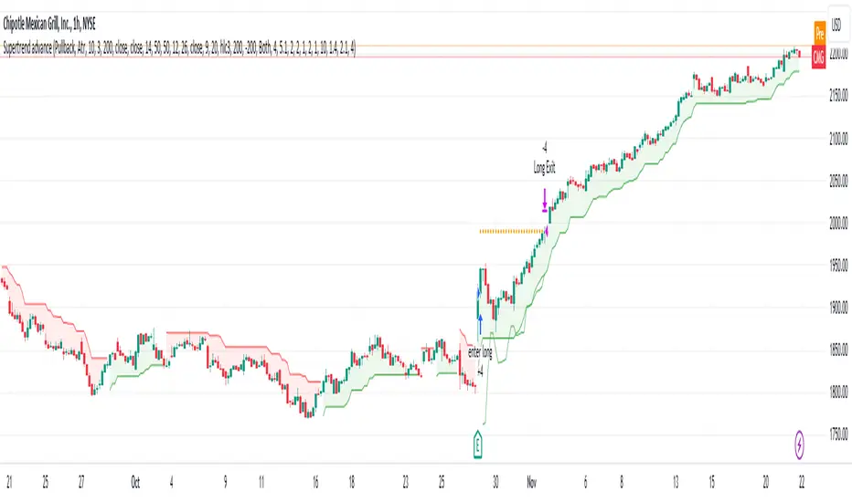
Liquidity Trading Algorithm (LTA)
The Liquidity Trading Algorithm is an algorithm designed to provide trade signals based on
liquidity conditions in the market. The underlying algorithm is based on the Liquidity
Dependent Price Movement (LDPM) metric and the Liquidity Dependent Price Stability (LDPS)
algorithm.
Together, LDPM and LDPS demonstrate statistically significant forecasting capabilities for price-
action on equities, cryptocurrencies, and futures. LTA takes these liquidity measurements and
translates them into actionable insights by way of entering or exiting a position based
on the future outlooks, as measured by the current liquidity status.
The benefit of LTA is that it can incorporate these powerful liquidity measurements into
actionable insights with several features designed to help you tailor LTA's behavior and
measurements to your desired vantage point. These customizable features come by the way of determining LTA's assessment style, and additional monitoring systems for avoiding bear and bull traps, along with various other quality of life features, discussed in more detail below.
First, a few quick facts:
- LTA is compatible on a wide array of instruments, including Equities, Futures, Cryptocurrencies, and Forex.
- LTA is compatible on most intervals in so long as the data can be calculated appropriately,
(be sure to do a backtest on timescales less than 1-minue to ensure the data can be computed).
- LTA only measures liquidity at the end of the interval of the chart chosen, and does not respond to conditions during the candle interval, unless specified (such as with `Stops`).
- LTA is interval-dependent, this means it will measure and behave differently on different
intervals as the underlying algorithms are dependent on the interval chosen.
- LTA can utilize fractional share sizing for cryptocurrencies.
- LTA can be restricted to either bullish or bearish indications.
- Additional Monitoring Systems are available for additional risk mitigation.
In short, LTA is a widely applicable, unique algorithm designed to translate liquidity measurements into liquidity insights.
Before getting more into the details, here is a quick list of the main features and settings
available for customization:
- Backtesting Start Date: Manual selection of the start date for the algorithm during backtesting.
- Assessment Style: adjust how LDPM and LDPS measure and respond to changes in liquidity.
- Impose Wait: force LTA to wait before entering or exiting a position to ensure conditions have remained conducive.
- Trade Direction Allowance: Restrict LTA to only long or only short, if desired.
- Position Sizing Method: determine how LTA calculates position sizing.
- Fractional Share Sizing: allow LTA to calculate fractional share sizes for cryptocurrencies
- Max Size Limit: Impose a maximum size on LTA's positions.
- Initial Capital: Indicate how much capital LTA should stat with.
- Portfolio Allotment: Indicate to LTA how much (in percentages) of the available balance should be considered when calculating position size.
- Enact Additional Monitoring Systems: Indicate if LTA should impose additional safety criteria when monitoring liquidity.
- Configure Take Profit, Stop-Loss, Trailing Stop Loss
- Display Information tables on the current position, overall strategy performance, along
with a text output showing LTA's processes.
- Real-time text output and updates on LTA's inner workings.
Let's get into some more of the details.
LTA's Assessment Style
LTA's assessment style determines how LTA collects and responds to changing data. In traditional terms, this is akin to (but not quite exactly the same as) the sensitivity versus specificity spectrum, whereby on one end (the sensitive end), an algorithm responds to changes in data in a reactive manner (which tends to lower its specificity, or how often it is correct in its indications), and on the other end, the opposite one, the algorithm foresakes quick changes for longevity of outlook.
While this is in part true, it is not a full view of the underlying mechanisms that changing the assessment style augments. A better analogy would be that the sensitive end of the spectrum (`Aggressive`) is in a state such that the algorithm wants to changing its outlooks, and as such, with changes in data, the algorithm has to be convinced as to why that is not a good idea to change outlooks, whereas the the more specific states (`Conservative`, `Diamond`) must be convinced that their view is no longer valid and that it needs to be changed.
This means the `Aggressive` and the `Diamond` settings fundamentally differ not just in their
data collection, but also in the data processing such that the `Aggressive` decision tree has to
be convinced that the data is the same (as its defualt is that it has changed),
and the `Diamond` decision tree has to be convinced that the data is not the same, and as such, the outlook need changed.
From there, the algorithm cooks through the data and determines to what the outlook should be changed to, given the current state of liquidity.
`Balanced` lies in the middle of this balance, attempting to balance being open to new ideas while not removing the wisdom of the past, as it were.
On a scale of most `sensitive` to most `specific`, it is as follows: `Aggressive`, `Balanced`,
`Conservative`, `Diamond`.
Functionally, these different modes can help in different liquidity environments, as certain
environments are more conducive to an eager approach (such as found near `Aggressive`) or are more conducive to a more conservative approach, where sudden changes in liquidity are known to be short-lived and unremarkable (such as many previously identified bull or bear traps).
For instance, on low interval views, it can often-times be beneficial to keep the algorithm towards the `Sensitive` end, since on the lower-timeframes, the crosswinds can change quite dramatically; whereas on the longer intervals, it may be useful to maintain a more `Specific` algorithm (such as found near `Diamond` mode) setting since longer intervals typically lend themselves to longer time-horizons, which themselves typically lend themselves to "weathering the storm", as it were.
LTA's Assessment Style is also supported by the Additional Monitoring Systems which works
to add sensitivity without sacrificing specificity by enacting a separate monitoring system, as described below.
Additional Monitoring Systems
The Additional Monitoring System (AMS) attempts to add more context to any changes in liquidity conditions as measured, such that LTA as a whole will have an expanded view into any rapidly changing liquidity conditions before these changes manifest in the traditional data streams. The ideal is that this allows for early exits or early entrances to positions "a head of time".
The traditional use of this system is to indicate when liquidity is suggestive of the end of a particular run (be it a bear run or a bull run), so an early exit can be initiated (and thus,
downside averted) even before the data officially showcase such changes. In such cases (when AMS becomes activated), the algorithm will signal to exit any open positions, and will restrict the opening of any new positions.
When a position is exited because of AMS, it is denoted as an `Early Exit` and if a position is prevented from being entered, the text output will display `AM prevented entry...` to indicate that conditions are not meeting AMS' additional standards.
The algorithm will wait to make any actions while `AMS` is `active` and will only enter into a new position once `AMS` has been `deactivated` and overall liquidity conditions are appropriate.
Functionally, the benefits of AMS translate to:
- Toggeling AMS on will typically see a net reduction in overall profitability, but
- AMS will typically (almost always) reduce max drawdown,
an increases in max runup, and increase return-over-maxdrawdown, and
- AMS can provide benefit for equities that experience a lot of "traps" by navigating early
entrance and early exits.
So in short, AMS is way of adding an additional level of liquidity monitoring that attempts to
exit positions if conditions look to be deteriorating, and to enter conditions if they look to be
improving. The cost of this additional monitoring, however, is a greater number of trades indicated, and a lower overall profitability.
Impose Wait
Note: `Impose Wait` will not force Take Profit, Stop Loss, or Trailing Stop Loss to
wait.
LTA can be indicated to `wait` before entering or exiting a position if desired. This means that if conditions change, whereas without a `wait` imposed, the algorithm would immediately indicate this change via a signal to alter the strategy's position, with a `wait` imposed, the algorithm will `wait` the indicated number of bars, and then re-check conditions before proceeding.
If, while waiting, conditions change to a state that is no longer compatible with the "order-in-
waiting", then the order-in-waiting is removed, and the counts reset (i.e.: conditions must remain favorable to the intended positional change throughout the wait period).
Since LTA works at the end-of-intervals, there is an inherently "built-in" wait of 1 bar when
switching directly from long to short (i.e.: if a full switch is indicated, then it is indicated as
conditions change -> exit new position -> wait until -> check conditions ->
enter new position as indicated). Thus, to impose a wait of `1 bar` would be to effectively have a total of two candles' ends prior to the entrance of the new position).
There are two main styles of `Impose Wait` that you can utilize:
- `Wait` : this mode will cause LTA to `wait` when both entering and exiting a position (in so long as it is not an exit signaled via a Take Profit, Stop Loss or Trailing Stop Loss).
- `Exit-Wait` : This mode will >not< cause LTA to `wait` if conditions require the closing of a position, but will force LTA to wait before entering into a position.
Position:
In addition to the availability to restrict LTA to either a long-only or short-only strategy, LTA
also comprises additional flexibility when deciding on how it should navigate the markets with
regards to sizing. Notably, this flexibility benefits several aspects of LTA's existence, namely the ability to determine the `Sizing Method`, or if `Fractional Share Sizing` should be employed, and more, as discussed below.
Position Sizing Method
There are two main ways LTA can determine the size of a position. Either via the `Fixed-Share` choice, or the `Fixed-Percentage` choice.
- `Fixed-Share` will use the amount indicated in the `Max Sizing Limit` field as the position size, always.
Note: With `Fixed-Share` sizing, LTA will >not< check if the balance is sufficient
prior to signaling an entrance.
- `Fixed-Percentage` will use the percentage amount indicated in the `Portfolio Allotment` field as the percentage of available funds to use when calculating the position size. Additionally, with the `Fixed-Percentage` choice, you can set the `Max Sizing Limit` if desired, which will ensure that no position will be entered greater than the amount indicated in the field.
Fractional Share Sizing
If the underlying instrument supports it (typically only cryptocurrencies), share sizing can be
fractionalized. If this is done, the resulting positin size is rounded to `4 digits`. This means any
position with a size less than `0.00005` will be rounded to `0.0000`
Note: Ensure that the underlying instrument supports fractional share sizing prior
to initiating.
Max Sizing Limit
As discussed above, the `Max Sizing Limit` will determine:
- The position size for every position, if `Sizing Method : Fixed-Share` is utilized, or
- The maximum allowed size, regardless of available capital, if `Sizing Method : Fixed-Percentage` is utilized.
Note: There is an internal maximum of 100,000 units.
Initial Capital
Note: There are 2 `Initial Capital` settings; one in LTA's settings and one in the
`Properties` tab. Ensure these two are the same when doing backtesting.
The initial capital field will be used to determine the starting balanace of the strategy, and
is used to calculate the internal data reporting (the data tables).
Portfolio Allotment
You can specify how much of the total available balance should be used when calculating the share size. The default is 100%.
Stops
Note: Stops over-ride `AMS` and `Impose Wait`, and are not restricted to only the
end-of-candle and will occur instantaneously upon their activation. Neither `AMS` nor `Impose Wait` can over-ride a signal from a `Take-Profit`, `Stop-Loss`, or a `Trailing-Stop Loss`.
LTA enhouses three stops that can be configured, a `Take-Profit`, a `Stop-Loss` and a `Trailing-Stop Loss`. The configurations can be set in the settings in percent terms. These exit signals will always over-ride AMS or any other restrictions on position exit.
Their configuration is rather standard; set the percentages you want the signal to be sent at and so it will be done.
Some quick notes on the `Trailing-Stop Loss`:
- The activation percentage must be reached (in profits) prior to the `Traililng-Stop Loss`
from activating the downside protection. For example, if the `Activation Percentage` is 10%, then unless the position reaches (at any point) a 10% profit, then it will not signal any exits on the downside, should it occur.
- The downside price-point is continuously updated and is calculated from the maximum profit reached in the given position and the loss percentage placed in the appropriate field.
Data Tables and Data Output
LTA provides real-time data output through a variety of mechanisms:
- `Position Table`
The `Position Table` displays information about the current position, including:
> Position Duration : how long the position has been open for.
> Indicates if the side is Long or Short, depending on if it is long or short.
> Entry Price: the price the position was entered at.
> Current Price (% Dif): the current price of the underlying and the %-difference between the entry price and the current price.
> Max Profit ($/%): the maximum profit reached in $ and % terms.
> Current PnL ($/%) : the current PnL for the open position.
- `Performance Table`
The `Performance Table` displays information regarding the overall performance of the algorithm since its `Start Date`. These data include:
> Initial Equity ($): The initial equity the algorithm started with.
> Current Equity ($): The current total equity of the account (including open positions)
> Net Profits ($|%) : The overall net profit in $ and % terms.
> Long / Short Trade Counts: The respective trade counts for the positions entered.
> Total Closed Trades: The running sum of the number of trades closed.
> Profitability: The calculation of the number of profitable trades over the total number of
trades.
> Avg. Profit / Trade: The calculation of the average profit per trade in both $ and % terms.
> Avg. Loss / Trade: The calculation of the average loss per trade in both $ and % terms.
> Max Run-Up: The maximum run-up the algorithm has seen in both $ and % terms.
> Max Drawdown: The maximum draw-down the algorithm has seen in both $ and % terms.
> Return-Over-Max-Drawdown: the ratio of the maximum drawdown against the current net profits.
- `Text Output`
LTA will output, if desired, signals to the text output field every time it analysis or performs and action. These messages can include information such as:
"
08:00:00 >> AM Protocol activated ... exiting position ...
08:00:00 >> Exit Order Created for qty: 2, profit: 380 (4.34%)
...
09:30:00 >> Checking conditions ...
09:30:00 >> AM protocol prevented entry ... waiting ...
"
This way, you can keep an eye out on what is happening "under the hood", as it were.
LTA will produce a message at the end of its assessment at the end of each candle interval, as well as when a position is exited due to a `Stop` or due to `AMS` being activated.
Additionally, the `Text Output` includes a initial message, but for space-constraints, this
can be toggled off with the `Blank Text Output` option within LTA's configurations.
For additional information, please refer to the Author's Instructions below.

Uhl MA System - Strategy AnalysisThe Uhl MA crossover system was specifically designed to provide an adaptive MA crossover system that didn't committed the same errors of more classical MA systems. This crossover system is based on a fast and a slow moving average, with the slow moving average being the corrected moving average (CMA) originally proposed by Andreas Uhl, and the fast moving average being the corrected trend step (CTS) which is also based on the corrected moving average design.
For more information see :
In this post, the performances of this system are analyzed on various markets.
Setup And Rules
The analysis is solely based on the indicator signals, therefore no spread is applied. Constant position sizing is used. The strategy will be backtested on the 15 minute time-frame. The mult setting is discarded, the default setting used for length is 100.
Here are the rules of our strategy :
long: CTS crossover CMA
short: CTS crossunder CMA
Results And Data
EURUSD:
Net Profit: $ 0.08
Total number of trades: 99
Profitability: 35.35 %
Profit Factor: 1.834
Max Drawdown: $ 0.01
EURUSD behaved pretty well, and was most of time showing long term trends without exhibiting particularly tricky structures, the moving averages still did cross during ranging phases, since march 9 we can see a downtrend with more pronounced cyclical variations (retracements) that could potentially lead to loosing trades.
BTCUSD:
Net Profit: $ 4371.57
Total number of trades: 94
Profitability: 32.98 %
Profit Factor: 1.749
Max Drawdown: $ 1409.96
The strategy didn't started well, producing its largest drawdown after only a few trades, the strategy still managed to recover. BTCUSD exhibited a strong downtrend, the strategy profited from that to recover, signals still occurred on ranging phases, and where mostly caused by a short term volatile move, unfortunately the CMA can converge toward ranging/flat price zones where false signals might occur at higher frequency.
AMD:
Net Profit: $ 16.09
Total number of trades: 95
Profitability: 29.47 %
Profit Factor: 1.288
Max Drawdown: $ 20.11
On AMD the strategy started relatively well with a raising balance, then the balance quickly fallen, this downtrend in the balance lasted quite some time (almost 48 trades), the strategy finally recovered in Nov 2019 and the balance made a new highest high at the end of February. AMD had numerous trends during the backtesting period, yet results are poor.
AAPL:
Net Profit: $ -28.17
Total number of trades: 89
Profitability: 28.09 %
Profit Factor: 0.894
Max Drawdown: $ 63.21
AAPL show the poorest results so far, with a stationary balance around the initial capital (in short the evolution of the balance is not showing any particular trend and oscillate around the initial capital value).
AAPL had some significant retracements in its up-trend, which triggered some trades (of course), and the ranging period from Jan 24 to Feb 13 heavily damaged the strategy performance, generating 6 significant loosing trades. AAPL show the worst results so far, mostly due by ranging phases.
Conclusions
The Uhl MA crossover system strategy has been tested and based on the results don't show particularly interesting performances, and might even be outperformed by simpler MA systems that prove to be more robust against ranging markets. The total number of executed trades are on average 94, and the profitability is on average 31%. The strategy might prove more interesting if we can correct the behavior of the CMA, who sometimes converged toward ranging/flat markets.
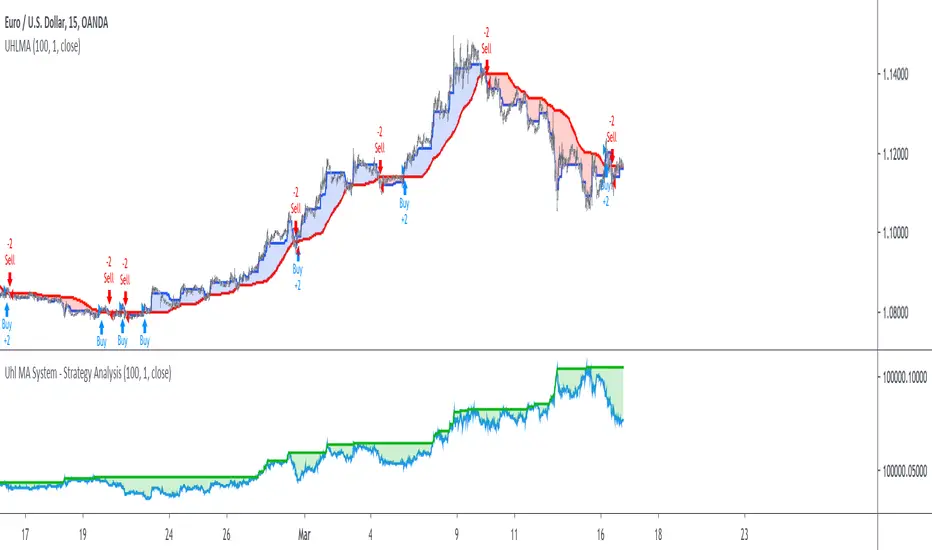
Destroyer LifeDestroyer Life Strategy - High-Frequency Long & Short Trading
Overview:
The Destroyer Life strategy is an advanced cryptocurrency trading algorithm designed for high-frequency execution on the 15-second timeframe. It combines CRT (Candle Range Trend) and Turtle Soup trading logic with multi-timeframe analysis to optimize entries and exits for both long and short trades. This strategy is specifically optimized for high-volatility crypto pairs, such as SOL/USD on MEXC, ensuring precise execution with minimal drawdown.
Key Features:
15-Second Timeframe Execution: Optimized for ultra-short-term trading.
Long & Short Strategy: Simultaneously identifies profitable buy and sell opportunities.
CRT & Turtle Soup Logic: Leverages price action patterns for enhanced trade accuracy.
Higher Timeframe Analysis (HTF): Incorporates liquidity zones, fair value gaps (FVG), and breaker blocks for context-aware trading.
Dynamic Position Sizing: Uses an adjustable leverage multiplier for risk-controlled trade sizing.
Commission Optimization: Ensures profitability even with trading fees.
Strict Risk Management: Implements exit conditions based on liquidity structure and trend reversals.
Strategy Performance (Backtested on SOL/USD - MEXC):
Overall Profitability: ~80% win rate in backtesting.
Net Profit: $3,151.12 (6.30% ROI).
Gross Profit: $3,795.68 (7.59%).
Gross Loss: $644.56 (1.29%).
Long Trades Profit: $1,459.05 (2.92%).
Short Trades Profit: $1,692.07 (3.38%).
Commission Paid: $924.82.
Minimum Trade Holding Period: 1-minute cooldown between trades.
Trading Logic:
Entry Conditions:
Long Trades: Triggered when the price enters a liquidity void and aligns with higher timeframe bullish bias.
Short Trades: Triggered when price approaches a resistance level with bearish higher timeframe confluence.
CRT & Turtle Soup Patterns: Identifies reversals by analyzing breakout and fake-out structures.
Exit Conditions:
Long Positions Close: Upon price exceeding a 3.88% profit threshold or reversing below an HTF structure.
Short Positions Close: Upon reaching a similar 3.88% threshold or showing strong bullish signals.
Dynamic Position Sizing:
Uses a leverage-based calculation that adapts trade size based on volatility.
Liquidity Awareness:
Tracks Mitigation Blocks (MB), Fair Value Gaps (FVG), Buy/Sell-Side Liquidity (BSL/SSL) to determine optimal execution.
Best Use Cases:
Scalpers & High-Frequency Traders: Those looking for rapid trade execution with short holding periods.
Crypto Traders Focused on Low Timeframes: Optimized for 15-second price action.
Traders Utilizing Liquidity Concepts: Built to exploit liquidity traps and inefficiencies.
Risks & Considerations:
High-Frequency Execution Requires Low Latency: Ensure your broker or exchange supports fast order execution.
Backtested Results May Vary: Real-time performance depends on market conditions.
Commission & Fees Impact Profits: Consider exchanges with low fees to maximize strategy efficiency.
Final Thoughts:
The Destroyer Life Strategy is designed for serious traders looking to take advantage of high-volatility markets with a structured, liquidity-based approach. By combining price action, liquidity concepts, and adaptive risk management, it provides a solid framework for executing high-probability trades on crypto markets.
🚀 Ready to take your trading to the next level? Try Destroyer Life today and dominate the markets!
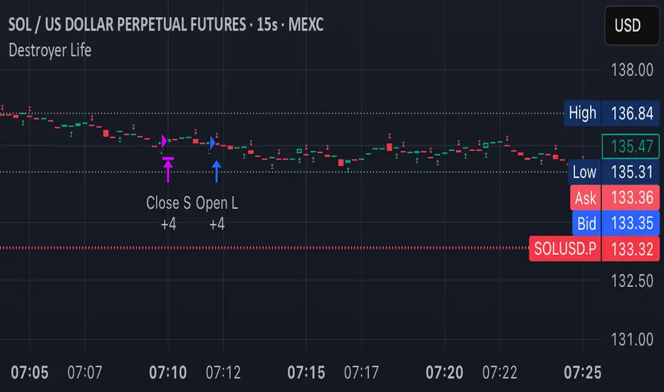
Dskyz (DAFE) Adaptive Regime - Quant Machine ProDskyz (DAFE) Adaptive Regime - Quant Machine Pro:
Buckle up for the Dskyz (DAFE) Adaptive Regime - Quant Machine Pro, is a strategy that’s your ultimate edge for conquering futures markets like ES, MES, NQ, and MNQ. This isn’t just another script—it’s a quant-grade powerhouse, crafted with precision to adapt to market regimes, deliver multi-factor signals, and protect your capital with futures-tuned risk management. With its shimmering DAFE visuals, dual dashboards, and glowing watermark, it turns your charts into a cyberpunk command center, making trading as thrilling as it is profitable.
Unlike generic scripts clogging up the space, the Adaptive Regime is a DAFE original, built from the ground up to tackle the chaos of futures trading. It identifies market regimes (Trending, Range, Volatile, Quiet) using ADX, Bollinger Bands, and HTF indicators, then fires trades based on a weighted scoring system that blends candlestick patterns, RSI, MACD, and more. Add in dynamic stops, trailing exits, and a 5% drawdown circuit breaker, and you’ve got a system that’s as safe as it is aggressive. Whether you’re a newbie or a prop desk pro, this strat’s your ticket to outsmarting the markets. Let’s break down every detail and see why it’s a must-have.
Why Traders Need This Strategy
Futures markets are a gauntlet—fast moves, volatility spikes (like the April 28, 2025 NQ 1k-point drop), and institutional traps that punish the unprepared. Meanwhile, platforms are flooded with low-effort scripts that recycle old ideas with zero innovation. The Adaptive Regime stands tall, offering:
Adaptive Intelligence: Detects market regimes (Trending, Range, Volatile, Quiet) to optimize signals, unlike one-size-fits-all scripts.
Multi-Factor Precision: Combines candlestick patterns, MA trends, RSI, MACD, volume, and HTF confirmation for high-probability trades.
Futures-Optimized Risk: Calculates position sizes based on $ risk (default: $300), with ATR or fixed stops/TPs tailored for ES/MES.
Bulletproof Safety: 5% daily drawdown circuit breaker and trailing stops keep your account intact, even in chaos.
DAFE Visual Mastery: Pulsing Bollinger Band fills, dynamic SL/TP lines, and dual dashboards (metrics + position) make signals crystal-clear and charts a work of art.
Original Craftsmanship: A DAFE creation, built with community passion, not a rehashed clone of generic code.
Traders need this because it’s a complete, adaptive system that blends quant smarts, user-friendly design, and DAFE flair. It’s your edge to trade with confidence, cut through market noise, and leave the copycats in the dust.
Strategy Components
1. Market Regime Detection
The strategy’s brain is its ability to classify market conditions into five regimes, ensuring signals match the environment.
How It Works:
Trending (Regime 1): ADX > 20, fast/slow EMA spread > 0.3x ATR, HTF RSI > 50 or MACD bullish (htf_trend_bull/bear).
Range (Regime 2): ADX < 25, price range < 3% of close, no HTF trend.
Volatile (Regime 3): BB width > 1.5x avg, ATR > 1.2x avg, HTF RSI overbought/oversold.
Quiet (Regime 4): BB width < 0.8x avg, ATR < 0.9x avg.
Other (Regime 5): Default for unclear conditions.
Indicators: ADX (14), BB width (20), ATR (14, 50-bar SMA), HTF RSI (14, daily default), HTF MACD (12,26,9).
Why It’s Brilliant:
Regime detection adapts signals to market context, boosting win rates in trending or volatile conditions.
HTF RSI/MACD add a big-picture filter, rare in basic scripts.
Visualized via gradient background (green for Trending, orange for Range, red for Volatile, gray for Quiet, navy for Other).
2. Multi-Factor Signal Scoring
Entries are driven by a weighted scoring system that combines candlestick patterns, trend, momentum, and volume for robust signals.
Candlestick Patterns:
Bullish: Engulfing (0.5), hammer (0.4 in Range, 0.2 else), morning star (0.2), piercing (0.2), double bottom (0.3 in Volatile, 0.15 else). Must be near support (low ≤ 1.01x 20-bar low) with volume spike (>1.5x 20-bar avg).
Bearish: Engulfing (0.5), shooting star (0.4 in Range, 0.2 else), evening star (0.2), dark cloud (0.2), double top (0.3 in Volatile, 0.15 else). Must be near resistance (high ≥ 0.99x 20-bar high) with volume spike.
Logic: Patterns are weighted higher in specific regimes (e.g., hammer in Range, double bottom in Volatile).
Additional Factors:
Trend: Fast EMA (20) > slow EMA (50) + 0.5x ATR (trend_bull, +0.2); opposite for trend_bear.
RSI: RSI (14) < 30 (rsi_bull, +0.15); > 70 (rsi_bear, +0.15).
MACD: MACD line > signal (12,26,9, macd_bull, +0.15); opposite for macd_bear.
Volume: ATR > 1.2x 50-bar avg (vol_expansion, +0.1).
HTF Confirmation: HTF RSI < 70 and MACD bullish (htf_bull_confirm, +0.2); RSI > 30 and MACD bearish (htf_bear_confirm, +0.2).
Scoring:
bull_score = sum of bullish factors; bear_score = sum of bearish. Entry requires score ≥ 1.0.
Example: Bullish engulfing (0.5) + trend_bull (0.2) + rsi_bull (0.15) + htf_bull_confirm (0.2) = 1.05, triggers long.
Why It’s Brilliant:
Multi-factor scoring ensures signals are confirmed by multiple market dynamics, reducing false positives.
Regime-specific weights make patterns more relevant (e.g., hammers shine in Range markets).
HTF confirmation aligns with the big picture, a quant edge over simplistic scripts.
3. Futures-Tuned Risk Management
The risk system is built for futures, calculating position sizes based on $ risk and offering flexible stops/TPs.
Position Sizing:
Logic: Risk per trade (default: $300) ÷ (stop distance in points * point value) = contracts, capped at max_contracts (default: 5). Point value = tick value (e.g., $12.5 for ES) * ticks per point (4) * contract multiplier (1 for ES, 0.1 for MES).
Example: $300 risk, 8-point stop, ES ($50/point) → 0.75 contracts, rounded to 1.
Impact: Precise sizing prevents over-leverage, critical for micro contracts like MES.
Stops and Take-Profits:
Fixed: Default stop = 8 points, TP = 16 points (2:1 reward/risk).
ATR-Based: Stop = 1.5x ATR (default), TP = 3x ATR, enabled via use_atr_for_stops.
Logic: Stops set at swing low/high ± stop distance; TPs at 2x stop distance from entry.
Impact: ATR stops adapt to volatility, while fixed stops suit stable markets.
Trailing Stops:
Logic: Activates at 50% of TP distance. Trails at close ± 1.5x ATR (atr_multiplier). Longs: max(trail_stop_long, close - ATR * 1.5); shorts: min(trail_stop_short, close + ATR * 1.5).
Impact: Locks in profits during trends, a game-changer in volatile sessions.
Circuit Breaker:
Logic: Pauses trading if daily drawdown > 5% (daily_drawdown = (max_equity - equity) / max_equity).
Impact: Protects capital during black swan events (e.g., April 27, 2025 ES slippage).
Why It’s Brilliant:
Futures-specific inputs (tick value, multiplier) make it plug-and-play for ES/MES.
Trailing stops and circuit breaker add pro-level safety, rare in off-the-shelf scripts.
Flexible stops (ATR or fixed) suit different trading styles.
4. Trade Entry and Exit Logic
Entries and exits are precise, driven by bull_score/bear_score and protected by drawdown checks.
Entry Conditions:
Long: bull_score ≥ 1.0, no position (position_size <= 0), drawdown < 5% (not pause_trading). Calculates contracts, sets stop at swing low - stop points, TP at 2x stop distance.
Short: bear_score ≥ 1.0, position_size >= 0, drawdown < 5%. Stop at swing high + stop points, TP at 2x stop distance.
Logic: Tracks entry_regime for PNL arrays. Closes opposite positions before entering.
Exit Conditions:
Stop-Loss/Take-Profit: Hits stop or TP (strategy.exit).
Trailing Stop: Activates at 50% TP, trails by ATR * 1.5.
Emergency Exit: Closes if price breaches stop (close < long_stop_price or close > short_stop_price).
Reset: Clears stop/TP prices when flat (position_size = 0).
Why It’s Brilliant:
Score-based entries ensure multi-factor confirmation, filtering out weak signals.
Trailing stops maximize profits in trends, unlike static exits in basic scripts.
Emergency exits add an extra safety layer, critical for futures volatility.
5. DAFE Visuals
The visuals are pure DAFE magic, blending function with cyberpunk flair to make signals intuitive and charts stunning.
Shimmering Bollinger Band Fill:
Display: BB basis (20, white), upper/lower (green/red, 45% transparent). Fill pulses (30–50 alpha) by regime, with glow (60–95 alpha) near bands (close ≥ 0.995x upper or ≤ 1.005x lower).
Purpose: Highlights volatility and key levels with a futuristic glow.
Visuals make complex regimes and signals instantly clear, even for newbies.
Pulsing effects and regime-specific colors add a DAFE signature, setting it apart from generic scripts.
BB glow emphasizes tradeable levels, enhancing decision-making.
Chart Background (Regime Heatmap):
Green — Trending Market: Strong, sustained price movement in one direction. The market is in a trend phase—momentum follows through.
Orange — Range-Bound: Market is consolidating or moving sideways, with no clear up/down trend. Great for mean reversion setups.
Red — Volatile Regime: High volatility, heightened risk, and larger/faster price swings—trade with caution.
Gray — Quiet/Low Volatility: Market is calm and inactive, with small moves—often poor conditions for most strategies.
Navy — Other/Neutral: Regime is uncertain or mixed; signals may be less reliable.
Bollinger Bands Glow (Dynamic Fill):
Neon Red Glow — Warning!: Price is near or breaking above the upper band; momentum is overstretched, watch for overbought conditions or reversals.
Bright Green Glow — Opportunity!: Price is near or breaking below the lower band; market could be oversold, prime for bounce or reversal.
Trend Green Fill — Trending Regime: Fills between bands with green when the market is trending, showing clear momentum.
Gold/Yellow Fill — Range Regime: Fills with gold/aqua in range conditions, showing the market is sideways/oscillating.
Magenta/Red Fill — Volatility Spike: Fills with vivid magenta/red during highly volatile regimes.
Blue Fill — Neutral/Quiet: A soft blue glow for other or uncertain market states.
Moving Averages:
Display: Blue fast EMA (20), red slow EMA (50), 2px.
Purpose: Shows trend direction, with trend_dir requiring ATR-scaled spread.
Dynamic SL/TP Lines:
Display: Pulsing colors (red SL, green TP for Trending; yellow/orange for Range, etc.), 3px, with pulse_alpha for shimmer.
Purpose: Tracks stops/TPs in real-time, color-coded by regime.
6. Dual Dashboards
Two dashboards deliver real-time insights, making the strat a quant command center.
Bottom-Left Metrics Dashboard (2x13):
Metrics: Mode (Active/Paused), trend (Bullish/Bearish/Neutral), ATR, ATR avg, volume spike (YES/NO), RSI (value + Oversold/Overbought/Neutral), HTF RSI, HTF trend, last signal (Buy/Sell/None), regime, bull score.
Display: Black (29% transparent), purple title, color-coded (green for bullish, red for bearish).
Purpose: Consolidates market context and signal strength.
Top-Right Position Dashboard (2x7):
Metrics: Regime, position side (Long/Short/None), position PNL ($), SL, TP, daily PNL ($).
Display: Black (29% transparent), purple title, color-coded (lime for Long, red for Short).
Purpose: Tracks live trades and profitability.
Why It’s Brilliant:
Dual dashboards cover market context and trade status, a rare feature.
Color-coding and concise metrics guide beginners (e.g., green “Buy” = go).
Real-time PNL and SL/TP visibility empower disciplined trading.
7. Performance Tracking
Logic: Arrays (regime_pnl_long/short, regime_win/loss_long/short) track PNL and win/loss by regime (1–5). Updated on trade close (barstate.isconfirmed).
Purpose: Prepares for future adaptive thresholds (e.g., adjust bull_score min based on regime performance).
Why It’s Brilliant: Lays the groundwork for self-optimizing logic, a quant edge over static scripts.
Key Features
Regime-Adaptive: Optimizes signals for Trending, Range, Volatile, Quiet markets.
Futures-Optimized: Precise sizing for ES/MES with tick-based risk inputs.
Multi-Factor Signals: Candlestick patterns, RSI, MACD, and HTF confirmation for robust entries.
Dynamic Exits: ATR/fixed stops, 2:1 TPs, and trailing stops maximize profits.
Safe and Smart: 5% drawdown breaker and emergency exits protect capital.
DAFE Visuals: Shimmering BB fill, pulsing SL/TP, and dual dashboards.
Backtest-Ready: Fixed qty and tick calc for accurate historical testing.
How to Use
Add to Chart: Load on a 5min ES/MES chart in TradingView.
Configure Inputs: Set instrument (ES/MES), tick value ($12.5/$1.25), multiplier (1/0.1), risk ($300 default). Enable ATR stops for volatility.
Monitor Dashboards: Bottom-left for regime/signals, top-right for position/PNL.
Backtest: Run in strategy tester to compare regimes.
Live Trade: Connect to Tradovate or similar. Watch for slippage (e.g., April 27, 2025 ES issues).
Replay Test: Try April 28, 2025 NQ drop to see regime shifts and stops.
Disclaimer
Trading futures involves significant risk of loss and is not suitable for all investors. Past performance does not guarantee future results. Backtest results may differ from live trading due to slippage, fees, or market conditions. Use this strategy at your own risk, and consult a financial advisor before trading. Dskyz (DAFE) Trading Systems is not responsible for any losses incurred.
Backtesting:
Frame: 2023-09-20 - 2025-04-29
Slippage: 3
Fee Typical Range (per side, per contract)
CME Exchange $1.14 – $1.20
Clearing $0.10 – $0.30
NFA Regulatory $0.02
Firm/Broker Commis. $0.25 – $0.80 (retail prop)
TOTAL $1.60 – $2.30 per side
Round Turn: (enter+exit) = $3.20 – $4.60 per contract
Final Notes
The Dskyz (DAFE) Adaptive Regime - Quant Machine Pro is more than a strategy—it’s a revolution. Crafted with DAFE’s signature precision, it rises above generic scripts with adaptive regimes, quant-grade signals, and visuals that make trading a thrill. Whether you’re scalping MES or swinging ES, this system empowers you to navigate markets with confidence and style. Join the DAFE crew, light up your charts, and let’s dominate the futures game!
(This publishing will most likely be taken down do to some miscellaneous rule about properly displaying charting symbols, or whatever. Once I've identified what part of the publishing they want to pick on, I'll adjust and repost.)
Use it with discipline. Use it with clarity. Trade smarter.
**I will continue to release incredible strategies and indicators until I turn this into a brand or until someone offers me a contract.
Created by Dskyz, powered by DAFE Trading Systems. Trade smart, trade bold.
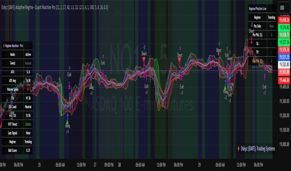
Buffett Quality Score [Consumer Discretionary]Evaluating Consumer Discretionary Companies with the Buffett Quality Score
The consumer discretionary sector, characterized by its sensitivity to economic cycles and consumer spending patterns, demands a robust framework for financial evaluation. The Buffett Quality Score offers a comprehensive assessment of financial health and performance specifically tailored to this dynamic industry. This scoring system combines critical financial ratios uniquely relevant to consumer discretionary companies, providing investors and analysts with a reliable tool for evaluation.
Selected Financial Metrics and Criteria
1. Altman Z-Score > 2.0
Relevance: The Altman Z-Score assesses bankruptcy risk, combining profitability, leverage, liquidity, solvency, and activity ratios. For consumer discretionary companies, which often face volatile market conditions, a score above 2.0 indicates financial stability and the ability to withstand economic downturns. This metric is particularly important in this sector due to the high variability in consumer spending.
2. Piotroski F-Score > 6.0
Relevance: The Piotroski F-Score evaluates fundamental strength based on profitability, leverage, liquidity, and operating efficiency. In the consumer discretionary sector, where rapid changes in consumer preferences can impact performance, a score above 6.0 highlights strong fundamental performance and resilience. This score is crucial for identifying companies with robust financial foundations in a highly competitive environment.
3. Asset Turnover > 1.0
Relevance: Asset Turnover measures the efficiency of asset use in generating sales. For consumer discretionary companies, a ratio above 1.0 signifies effective utilization of assets to drive revenue growth. Given the sector's reliance on high sales volumes and rapid inventory turnover, this metric is key to assessing operational efficiency.
4. Current Ratio > 1.5
Relevance: The Current Ratio assesses liquidity by comparing current assets to current liabilities. A ratio above 1.5 ensures that consumer discretionary companies can meet short-term obligations. This liquidity is essential for maintaining operational stability and flexibility to adapt to market changes, especially during economic fluctuations.
5. Debt to Equity Ratio < 1.0
Relevance: A lower Debt to Equity Ratio indicates prudent financial management and reduced reliance on debt. This is particularly important for consumer discretionary companies, which need to maintain financial flexibility to invest in new trends and innovations without overleveraging. Lower debt levels also reduce risk during economic downturns.
6. EBITDA Margin > 15.0%
Relevance: The EBITDA Margin measures operating profitability. A margin above 15.0% indicates efficient operations and the ability to generate sufficient earnings before interest, taxes, depreciation, and amortization. This is crucial for sustaining profitability in a competitive and fluctuating market, ensuring the company can reinvest in growth and innovation.
7. EPS One-Year Growth > 5.0%
Relevance: EPS growth reflects the company’s ability to increase earnings per share over the past year. For consumer discretionary companies, growth exceeding 5.0% signals positive earnings momentum, which is vital for investor confidence and the ability to fund future growth initiatives. This metric highlights companies that are successfully increasing profitability.
8. Gross Margin > 25.0%
Relevance: Gross Margin represents the profitability of sales after production costs. A margin exceeding 25.0% indicates strong pricing power and effective cost management, crucial for maintaining profitability while adapting to changing consumer demands. High gross margins are indicative of a company’s ability to control costs and price products competitively.
9. Net Margin > 10.0%
Relevance: Net Margin measures overall profitability after all expenses. A margin above 10.0% highlights the company’s ability to maintain strong profit levels, ensuring financial health and stability. This is essential for sustaining operations and investing in new opportunities, reflecting the company's efficiency in converting revenue into actual profit.
10.Return on Equity (ROE) > 15.0%
Relevance: ROE indicates how effectively a company uses equity to generate profits. An ROE above 15.0% signifies strong shareholder value creation. This metric is key for evaluating long-term performance in the consumer discretionary sector, where investor returns are closely tied to the company’s ability to innovate and grow. High ROE demonstrates effective management and profitable use of equity capital.
Interpreting the Buffett Quality Score
0-4 Points: Indicates potential weaknesses across multiple financial areas, warranting further investigation and risk assessment.
5 Points: Suggests average performance based on sector-specific criteria, indicating a need for cautious optimism.
6-10 Points: Signifies strong financial health and quality, meeting or exceeding most performance thresholds, making the company a potentially attractive investment.
Conclusion
The Buffett Quality Score provides a structured approach to evaluating financial health and performance. By focusing on these essential financial metrics, stakeholders can make informed decisions, identifying companies that are well-positioned to thrive in the competitive and economically sensitive consumer discretionary sector.
Disclaimer: The Buffett Quality Score serves as a tool for financial evaluation and analysis. It is not a substitute for professional financial advice or investment recommendations. Investors should conduct thorough research and seek personalized guidance based on individual circumstances.

[Joy] Jasmine Strategy for Bitcoin and CryptoIt is my strategy I use for spot and future trading, mostly for BTCUSD
Notable parameters used:
INDEX:BTCUSD
Data: 2017 - today
Long trade margin/leverage: 8x (50/8 = 6.25)
Short trade margin/leverage: 1x (50/50 = 1)
Commission: 0.075%
Initial Capital: $15, 000
Results:
Net profit: 832.74 %
Buy & Hold: 602.56 %. It beats the buy and hold.
Percent profitability: 88 % . It means 8 out of 10 trades resulted in profits.
Margin Calls: 0 (i.e. Never had a margin call according to backtest from 2017 till today)
Total closes trades: 25
Profit factor: 8.238
Avg Winning Trade: 43.08 %
Largest Winning Trade: 334.85 %
Avg # Bars in Winning Trades: 44 (i.e. 88 days)
Sharpe Ratio: 0.61. A Sharpe ratio under 1.0 is considered sub-optimal. Because of the big swings, I cannot make the Sharpe ratio any better at this time.
Sortino Ratio: 5.153. I think a Sortino ratio of 3.0 or higher is considered excellent. Do your research.
I am using 7.1% stop loss on long trades. However, you can turn off the stop loss and note the profitability remains the same.
Do remember there may be other costs, such as funding costs.
Description:
The strategy hunts for a few market features, namely breakouts, abnormal wicks relative to the body, abnormal volume relative to the candle characteristics, and possible confirmation of all these. It also hunts for more aspects. It gives a relative score of each of the characteristics. Finally, it tries to draw a guesstimate. In the end, it is only a guesstimate. Users see the final outcome (buy/sell etc). The whole logic happens at the background.
The strategy is not to be used for scalping, day trading or swing trading. In other words, it is not suitable for trading in a lower timeframe. It is to be used for Positional Trading For example, if one is trying this for BTCUSD, one may only try this for BTCUSD in a 2day timeframe and not in lower timeframes (such as 4 hours or 1 hour etc.) I am primarily interested in BTC for my research. However, it may be tested on other cryptos as well with varying degrees of results.
Please remember that past performance does not be indicative of future results. Different types of investments involve varying degrees of risk. There can be no assurance that the information referred to directly or indirectly in this strategy will be profitable, equal to any corresponding historical performance level(s), or suitable for you in any form or shape. Market condition changes very fast. Moreover, it would be best if you did not assume that any discussion or information contained here serves as the receipt of, or as a substitute for, personalized investment advice. I am not a financial advisor. I have no qualifications to be a financial advisor. It is only for educational and research purposes. Readers are encouraged to consult with a professional advisor of his/her choosing. Neither I nor my indicators or strategies take any responsibility for any misuse of the information for any actual trading. Even though this strategy did 88% profitability from 2017-2021, it may do poorly and may even be NOT profitable in the future.

Backtesting & Trading Engine [PineCoders]The PineCoders Backtesting and Trading Engine is a sophisticated framework with hybrid code that can run as a study to generate alerts for automated or discretionary trading while simultaneously providing backtest results. It can also easily be converted to a TradingView strategy in order to run TV backtesting. The Engine comes with many built-in strats for entries, filters, stops and exits, but you can also add you own.
If, like any self-respecting strategy modeler should, you spend a reasonable amount of time constantly researching new strategies and tinkering, our hope is that the Engine will become your inseparable go-to tool to test the validity of your creations, as once your tests are conclusive, you will be able to run this code as a study to generate the alerts required to put it in real-world use, whether for discretionary trading or to interface with an execution bot/app. You may also find the backtesting results the Engine produces in study mode enough for your needs and spend most of your time there, only occasionally converting to strategy mode in order to backtest using TV backtesting.
As you will quickly grasp when you bring up this script’s Settings, this is a complex tool. While you will be able to see results very quickly by just putting it on a chart and using its built-in strategies, in order to reap the full benefits of the PineCoders Engine, you will need to invest the time required to understand the subtleties involved in putting all its potential into play.
Disclaimer: use the Engine at your own risk.
Before we delve in more detail, here’s a bird’s eye view of the Engine’s features:
More than 40 built-in strategies,
Customizable components,
Coupling with your own external indicator,
Simple conversion from Study to Strategy modes,
Post-Exit analysis to search for alternate trade outcomes,
Use of the Data Window to show detailed bar by bar trade information and global statistics, including some not provided by TV backtesting,
Plotting of reminders and generation of alerts on in-trade events.
By combining your own strats to the built-in strats supplied with the Engine, and then tuning the numerous options and parameters in the Inputs dialog box, you will be able to play what-if scenarios from an infinite number of permutations.
USE CASES
You have written an indicator that provides an entry strat but it’s missing other components like a filter and a stop strategy. You add a plot in your indicator that respects the Engine’s External Signal Protocol, connect it to the Engine by simply selecting your indicator’s plot name in the Engine’s Settings/Inputs and then run tests on different combinations of entry stops, in-trade stops and profit taking strats to find out which one produces the best results with your entry strat.
You are building a complex strategy that you will want to run as an indicator generating alerts to be sent to a third-party execution bot. You insert your code in the Engine’s modules and leverage its trade management code to quickly move your strategy into production.
You have many different filters and want to explore results using them separately or in combination. Integrate the filter code in the Engine and run through different permutations or hook up your filtering through the external input and control your filter combos from your indicator.
You are tweaking the parameters of your entry, filter or stop strat. You integrate it in the Engine and evaluate its performance using the Engine’s statistics.
You always wondered what results a random entry strat would yield on your markets. You use the Engine’s built-in random entry strat and test it using different combinations of filters, stop and exit strats.
You want to evaluate the impact of fees and slippage on your strategy. You use the Engine’s inputs to play with different values and get immediate feedback in the detailed numbers provided in the Data Window.
You just want to inspect the individual trades your strategy generates. You include it in the Engine and then inspect trades visually on your charts, looking at the numbers in the Data Window as you move your cursor around.
You have never written a production-grade strategy and you want to learn how. Inspect the code in the Engine; you will find essential components typical of what is being used in actual trading systems.
You have run your system for a while and have compiled actual slippage information and your broker/exchange has updated his fees schedule. You enter the information in the Engine and run it on your markets to see the impact this has on your results.
FEATURES
Before going into the detail of the Inputs and the Data Window numbers, here’s a more detailed overview of the Engine’s features.
Built-in strats
The engine comes with more than 40 pre-coded strategies for the following standard system components:
Entries,
Filters,
Entry stops,
2 stage in-trade stops with kick-in rules,
Pyramiding rules,
Hard exits.
While some of the filter and stop strats provided may be useful in production-quality systems, you will not devise crazy profit-generating systems using only the entry strats supplied; that part is still up to you, as will be finding the elusive combination of components that makes winning systems. The Engine will, however, provide you with a solid foundation where all the trade management nitty-gritty is handled for you. By binding your custom strats to the Engine, you will be able to build reliable systems of the best quality currently allowed on the TV platform.
On-chart trade information
As you move over the bars in a trade, you will see trade numbers in the Data Window change at each bar. The engine calculates the P&L at every bar, including slippage and fees that would be incurred were the trade exited at that bar’s close. If the trade includes pyramided entries, those will be taken into account as well, although for those, final fees and slippage are only calculated at the trade’s exit.
You can also see on-chart markers for the entry level, stop positions, in-trade special events and entries/exits (you will want to disable these when using the Engine in strategy mode to see TV backtesting results).
Customization
You can couple your own strats to the Engine in two ways:
1. By inserting your own code in the Engine’s different modules. The modular design should enable you to do so with minimal effort by following the instructions in the code.
2. By linking an external indicator to the engine. After making the proper selections in the engine’s Settings and providing values respecting the engine’s protocol, your external indicator can, when the Engine is used in Indicator mode only:
Tell the engine when to enter long or short trades, but let the engine’s in-trade stop and exit strats manage the exits,
Signal both entries and exits,
Provide an entry stop along with your entry signal,
Filter other entry signals generated by any of the engine’s entry strats.
Conversion from strategy to study
TradingView strategies are required to backtest using the TradingView backtesting feature, but if you want to generate alerts with your script, whether for automated trading or just to trigger alerts that you will use in discretionary trading, your code has to run as a study since, for the time being, strategies can’t generate alerts. From hereon we will use indicator as a synonym for study.
Unless you want to maintain two code bases, you will need hybrid code that easily flips between strategy and indicator modes, and your code will need to restrict its use of strategy() calls and their arguments if it’s going to be able to run both as an indicator and a strategy using the same trade logic. That’s one of the benefits of using this Engine. Once you will have entered your own strats in the Engine, it will be a matter of commenting/uncommenting only four lines of code to flip between indicator and strategy modes in a matter of seconds.
Additionally, even when running in Indicator mode, the Engine will still provide you with precious numbers on your individual trades and global results, some of which are not available with normal TradingView backtesting.
Post-Exit Analysis for alternate outcomes (PEA)
While typical backtesting shows results of trade outcomes, PEA focuses on what could have happened after the exit. The intention is to help traders get an idea of the opportunity/risk in the bars following the trade in order to evaluate if their exit strategies are too aggressive or conservative.
After a trade is exited, the Engine’s PEA module continues analyzing outcomes for a user-defined quantity of bars. It identifies the maximum opportunity and risk available in that space, and calculates the drawdown required to reach the highest opportunity level post-exit, while recording the number of bars to that point.
Typically, if you can’t find opportunity greater than 1X past your trade using a few different reasonable lengths of PEA, your strategy is doing pretty good at capturing opportunity. Remember that 100% of opportunity is never capturable. If, however, PEA was finding post-trade maximum opportunity of 3 or 4X with average drawdowns of 0.3 to those areas, this could be a clue revealing your system is exiting trades prematurely. To analyze PEA numbers, you can uncomment complete sets of plots in the Plot module to reveal detailed global and individual PEA numbers.
Statistics
The Engine provides stats on your trades that TV backtesting does not provide, such as:
Average Profitability Per Trade (APPT), aka statistical expectancy, a crucial value.
APPT per bar,
Average stop size,
Traded volume .
It also shows you on a trade-by-trade basis, on-going individual trade results and data.
In-trade events
In-trade events can plot reminders and trigger alerts when they occur. The built-in events are:
Price approaching stop,
Possible tops/bottoms,
Large stop movement (for discretionary trading where stop is moved manually),
Large price movements.
Slippage and Fees
Even when running in indicator mode, the Engine allows for slippage and fees to be included in the logic and test results.
Alerts
The alert creation mechanism allows you to configure alerts on any combination of the normal or pyramided entries, exits and in-trade events.
Backtesting results
A few words on the numbers calculated in the Engine. Priority is given to numbers not shown in TV backtesting, as you can readily convert the script to a strategy if you need them.
We have chosen to focus on numbers expressing results relative to X (the trade’s risk) rather than in absolute currency numbers or in other more conventional but less useful ways. For example, most of the individual trade results are not shown in percentages, as this unit of measure is often less meaningful than those expressed in units of risk (X). A trade that closes with a +25% result, for example, is a poor outcome if it was entered with a -50% stop. Expressed in X, this trade’s P&L becomes 0.5, which provides much better insight into the trade’s outcome. A trade that closes with a P&L of +2X has earned twice the risk incurred upon entry, which would represent a pre-trade risk:reward ratio of 2.
The way to go about it when you think in X’s and that you adopt the sound risk management policy to risk a fixed percentage of your account on each trade is to equate a currency value to a unit of X. E.g. your account is 10K USD and you decide you will risk a maximum of 1% of it on each trade. That means your unit of X for each trade is worth 100 USD. If your APPT is 2X, this means every time you risk 100 USD in a trade, you can expect to make, on average, 200 USD.
By presenting results this way, we hope that the Engine’s statistics will appeal to those cognisant of sound risk management strategies, while gently leading traders who aren’t, towards them.
We trade to turn in tangible profits of course, so at some point currency must come into play. Accordingly, some values such as equity, P&L, slippage and fees are expressed in currency.
Many of the usual numbers shown in TV backtests are nonetheless available, but they have been commented out in the Engine’s Plot module.
Position sizing and risk management
All good system designers understand that optimal risk management is at the very heart of all winning strategies. The risk in a trade is defined by the fraction of current equity represented by the amplitude of the stop, so in order to manage risk optimally on each trade, position size should adjust to the stop’s amplitude. Systems that enter trades with a fixed stop amplitude can get away with calculating position size as a fixed percentage of current equity. In the context of a test run where equity varies, what represents a fixed amount of risk translates into different currency values.
Dynamically adjusting position size throughout a system’s life is optimal in many ways. First, as position sizing will vary with current equity, it reproduces a behavioral pattern common to experienced traders, who will dial down risk when confronted to poor performance and increase it when performance improves. Second, limiting risk confers more predictability to statistical test results. Third, position sizing isn’t just about managing risk, it’s also about maximizing opportunity. By using the maximum leverage (no reference to trading on margin here) into the trade that your risk management strategy allows, a dynamic position size allows you to capture maximal opportunity.
To calculate position sizes using the fixed risk method, we use the following formula: Position = Account * MaxRisk% / Stop% [, which calculates a position size taking into account the trade’s entry stop so that if the trade is stopped out, 100 USD will be lost. For someone who manages risk this way, common instructions to invest a certain percentage of your account in a position are simply worthless, as they do not take into account the risk incurred in the trade.
The Engine lets you select either the fixed risk or fixed percentage of equity position sizing methods. The closest thing to dynamic position sizing that can currently be done with alerts is to use a bot that allows syntax to specify position size as a percentage of equity which, while being dynamic in the sense that it will adapt to current equity when the trade is entered, does not allow us to modulate position size using the stop’s amplitude. Changes to alerts are on the way which should solve this problem.
In order for you to simulate performance with the constraint of fixed position sizing, the Engine also offers a third, less preferable option, where position size is defined as a fixed percentage of initial capital so that it is constant throughout the test and will thus represent a varying proportion of current equity.
Let’s recap. The three position sizing methods the Engine offers are:
1. By specifying the maximum percentage of risk to incur on your remaining equity, so the Engine will dynamically adjust position size for each trade so that, combining the stop’s amplitude with position size will yield a fixed percentage of risk incurred on current equity,
2. By specifying a fixed percentage of remaining equity. Note that unless your system has a fixed stop at entry, this method will not provide maximal risk control, as risk will vary with the amplitude of the stop for every trade. This method, as the first, does however have the advantage of automatically adjusting position size to equity. It is the Engine’s default method because it has an equivalent in TV backtesting, so when flipping between indicator and strategy mode, test results will more or less correspond.
3. By specifying a fixed percentage of the Initial Capital. While this is the least preferable method, it nonetheless reflects the reality confronted by most system designers on TradingView today. In this case, risk varies both because the fixed position size in initial capital currency represents a varying percentage of remaining equity, and because the trade’s stop amplitude may vary, adding another variability vector to risk.
Note that the Engine cannot display equity results for strategies entering trades for a fixed amount of shares/contracts at a variable price.
SETTINGS/INPUTS
Because the initial text first published with a script cannot be edited later and because there are just too many options, the Engine’s Inputs will not be covered in minute detail, as they will most certainly evolve. We will go over them with broad strokes; you should be able to figure the rest out. If you have questions, just ask them here or in the PineCoders Telegram group.
Display
The display header’s checkbox does nothing.
For the moment, only one exit strategy uses a take profit level, so only that one will show information when checking “Show Take Profit Level”.
Entries
You can activate two simultaneous entry strats, each selected from the same set of strats contained in the Engine. If you select two and they fire simultaneously, the main strat’s signal will be used.
The random strat in each list uses a different seed, so you will get different results from each.
The “Filter transitions” and “Filter states” strats delegate signal generation to the selected filter(s). “Filter transitions” signals will only fire when the filter transitions into bull/bear state, so after a trade is stopped out, the next entry may take some time to trigger if the filter’s state does not change quickly. When you choose “Filter states”, then a new trade will be entered immediately after an exit in the direction the filter allows.
If you select “External Indicator”, your indicator will need to generate a +2/-2 (or a positive/negative stop value) to enter a long/short position, providing the selected filters allow for it. If you wish to use the Engine’s capacity to also derive the entry stop level from your indicator’s signal, then you must explicitly choose this option in the Entry Stops section.
Filters
You can activate as many filters as you wish; they are additive. The “Maximum stop allowed on entry” is an important component of proper risk management. If your system has an average 3% stop size and you need to trade using fixed position sizes because of alert/execution bot limitations, you must use this filter because if your system was to enter a trade with a 15% stop, that trade would incur 5 times the normal risk, and its result would account for an abnormally high proportion in your system’s performance.
Remember that any filter can also be used as an entry signal, either when it changes states, or whenever no trade is active and the filter is in a bull or bear mode.
Entry Stops
An entry stop must be selected in the Engine, as it requires a stop level before the in-trade stop is calculated. Until the selected in-trade stop strat generates a stop that comes closer to price than the entry stop (or respects another one of the in-trade stops kick in strats), the entry stop level is used.
It is here that you must select “External Indicator” if your indicator supplies a +price/-price value to be used as the entry stop. A +price is expected for a long entry and a -price value will enter a short with a stop at price. Note that the price is the absolute price, not an offset to the current price level.
In-Trade Stops
The Engine comes with many built-in in-trade stop strats. Note that some of them share the “Length” and “Multiple” field, so when you swap between them, be sure that the length and multiple in use correspond to what you want for that stop strat. Suggested defaults appear with the name of each strat in the dropdown.
In addition to the strat you wish to use, you must also determine when it kicks in to replace the initial entry’s stop, which is determined using different strats. For strats where you can define a positive or negative multiple of X, percentage or fixed value for a kick-in strat, a positive value is above the trade’s entry fill and a negative one below. A value of zero represents breakeven.
Pyramiding
What you specify in this section are the rules that allow pyramiding to happen. By themselves, these rules will not generate pyramiding entries. For those to happen, entry signals must be issued by one of the active entry strats, and conform to the pyramiding rules which act as a filter for them. The “Filter must allow entry” selection must be chosen if you want the usual system’s filters to act as additional filtering criteria for your pyramided entries.
Hard Exits
You can choose from a variety of hard exit strats. Hard exits are exit strategies which signal trade exits on specific events, as opposed to price breaching a stop level in In-Trade Stops strategies. They are self-explanatory. The last one labelled When Take Profit Level (multiple of X) is reached is the only one that uses a level, but contrary to stops, it is above price and while it is relative because it is expressed as a multiple of X, it does not move during the trade. This is the level called Take Profit that is show when the “Show Take Profit Level” checkbox is checked in the Display section.
While stops focus on managing risk, hard exit strategies try to put the emphasis on capturing opportunity.
Slippage
You can define it as a percentage or a fixed value, with different settings for entries and exits. The entry and exit markers on the chart show the impact of slippage on the entry price (the fill).
Fees
Fees, whether expressed as a percentage of position size in and out of the trade or as a fixed value per in and out, are in the same units of currency as the capital defined in the Position Sizing section. Fees being deducted from your Capital, they do not have an impact on the chart marker positions.
In-Trade Events
These events will only trigger during trades. They can be helpful to act as reminders for traders using the Engine as assistance to discretionary trading.
Post-Exit Analysis
It is normally on. Some of its results will show in the Global Numbers section of the Data Window. Only a few of the statistics generated are shown; many more are available, but commented out in the Plot module.
Date Range Filtering
Note that you don’t have to change the dates to enable/diable filtering. When you are done with a specific date range, just uncheck “Date Range Filtering” to disable date filtering.
Alert Triggers
Each selection corresponds to one condition. Conditions can be combined into a single alert as you please. Just be sure you have selected the ones you want to trigger the alert before you create the alert. For example, if you trade in both directions and you want a single alert to trigger on both types of exits, you must select both “Long Exit” and “Short Exit” before creating your alert.
Once the alert is triggered, these settings no longer have relevance as they have been saved with the alert.
When viewing charts where an alert has just triggered, if your alert triggers on more than one condition, you will need the appropriate markers active on your chart to figure out which condition triggered the alert, since plotting of markers is independent of alert management.
Position sizing
You have 3 options to determine position size:
1. Proportional to Stop -> Variable, with a cap on size.
2. Percentage of equity -> Variable.
3. Percentage of Initial Capital -> Fixed.
External Indicator
This is where you connect your indicator’s plot that will generate the signals the Engine will act upon. Remember this only works in Indicator mode.
DATA WINDOW INFORMATION
The top part of the window contains global numbers while the individual trade information appears in the bottom part. The different types of units used to express values are:
curr: denotes the currency used in the Position Sizing section of Inputs for the Initial Capital value.
quote: denotes quote currency, i.e. the value the instrument is expressed in, or the right side of the market pair (USD in EURUSD ).
X: the stop’s amplitude, itself expressed in quote currency, which we use to express a trade’s P&L, so that a trade with P&L=2X has made twice the stop’s amplitude in profit. This is sometimes referred to as R, since it represents one unit of risk. It is also the unit of measure used in the APPT, which denotes expected reward per unit of risk.
X%: is also the stop’s amplitude, but expressed as a percentage of the Entry Fill.
The numbers appearing in the Data Window are all prefixed:
“ALL:” the number is the average for all first entries and pyramided entries.
”1ST:” the number is for first entries only.
”PYR:” the number is for pyramided entries only.
”PEA:” the number is for Post-Exit Analyses
Global Numbers
Numbers in this section represent the results of all trades up to the cursor on the chart.
Average Profitability Per Trade (X): This value is the most important gauge of your strat’s worthiness. It represents the returns that can be expected from your strat for each unit of risk incurred. E.g.: your APPT is 2.0, thus for every unit of currency you invest in a trade, you can on average expect to obtain 2 after the trade. APPT is also referred to as “statistical expectancy”. If it is negative, your strategy is losing, even if your win rate is very good (it means your winning trades aren’t winning enough, or your losing trades lose too much, or both). Its counterpart in currency is also shown, as is the APPT/bar, which can be a useful gauge in deciding between rivalling systems.
Profit Factor: Gross of winning trades/Gross of losing trades. Strategy is profitable when >1. Not as useful as the APPT because it doesn’t take into account the win rate and the average win/loss per trade. It is calculated from the total winning/losing results of this particular backtest and has less predictive value than the APPT. A good profit factor together with a poor APPT means you just found a chart where your system outperformed. Relying too much on the profit factor is a bit like a poker player who would think going all in with two’s against aces is optimal because he just won a hand that way.
Win Rate: Percentage of winning trades out of all trades. Taken alone, it doesn’t have much to do with strategy profitability. You can have a win rate of 99% but if that one trade in 100 ruins you because of poor risk management, 99% doesn’t look so good anymore. This number speaks more of the system’s profile than its worthiness. Still, it can be useful to gauge if the system fits your personality. It can also be useful to traders intending to sell their systems, as low win rate systems are more difficult to sell and require more handholding of worried customers.
Equity (curr): This the sum of initial capital and the P&L of your system’s trades, including fees and slippage.
Return on Capital is the equivalent of TV’s Net Profit figure, i.e. the variation on your initial capital.
Maximum drawdown is the maximal drawdown from the highest equity point until the drop . There is also a close to close (meaning it doesn’t take into account in-trade variations) maximum drawdown value commented out in the code.
The next values are self-explanatory, until:
PYR: Avg Profitability Per Entry (X): this is the APPT for all pyramided entries.
PEA: Avg Max Opp . Available (X): the average maximal opportunity found in the Post-Exit Analyses.
PEA: Avg Drawdown to Max Opp . (X): this represents the maximum drawdown (incurred from the close at the beginning of the PEA analysis) required to reach the maximal opportunity point.
Trade Information
Numbers in this section concern only the current trade under the cursor. Most of them are self-explanatory. Use the description’s prefix to determine what the values applies to.
PYR: Avg Profitability Per Entry (X): While this value includes the impact of all current pyramided entries (and only those) and updates when you move your cursor around, P&L only reflects fees at the trade’s last bar.
PEA: Max Opp . Available (X): It’s the most profitable close reached post-trade, measured from the trade’s Exit Fill, expressed in the X value of the trade the PEA follows.
PEA: Drawdown to Max Opp . (X): This is the maximum drawdown from the trade’s Exit Fill that needs to be sustained in order to reach the maximum opportunity point, also expressed in X. Note that PEA numbers do not include slippage and fees.
EXTERNAL SIGNAL PROTOCOL
Only one external indicator can be connected to a script; in order to leverage its use to the fullest, the engine provides options to use it as either an entry signal, an entry/exit signal or a filter. When used as an entry signal, you can also use the signal to provide the entry’s stop. Here’s how this works:
For filter state: supply +1 for bull (long entries allowed), -1 for bear (short entries allowed).
For entry signals: supply +2 for long, -2 for short.
For exit signals: supply +3 for exit from long, -3 for exit from short.
To send an entry stop level with an entry signal: Send positive stop level for long entry (e.g. 103.33 to enter a long with a stop at 103.33), negative stop level for short entry (e.g. -103.33 to enter a short with a stop at 103.33). If you use this feature, your indicator will have to check for exact stop levels of 1.0, 2.0 or 3.0 and their negative counterparts, and fudge them with a tick in order to avoid confusion with other signals in the protocol.
Remember that mere generation of the values by your indicator will have no effect until you explicitly allow their use in the appropriate sections of the Engine’s Settings/Inputs.
An example of a script issuing a signal for the Engine is published by PineCoders.
RECOMMENDATIONS TO ASPIRING SYSTEM DESIGNERS
Stick to higher timeframes. On progressively lower timeframes, margins decrease and fees and slippage take a proportionally larger portion of profits, to the point where they can very easily turn a profitable strategy into a losing one. Additionally, your margin for error shrinks as the equilibrium of your system’s profitability becomes more fragile with the tight numbers involved in the shorter time frames. Avoid <1H time frames.
Know and calculate fees and slippage. To avoid market shock, backtest using conservative fees and slippage parameters. Systems rarely show unexpectedly good returns when they are confronted to the markets, so put all chances on your side by being outrageously conservative—or a the very least, realistic. Test results that do not include fees and slippage are worthless. Slippage is there for a reason, and that’s because our interventions in the market change the market. It is easier to find alpha in illiquid markets such as cryptos because not many large players participate in them. If your backtesting results are based on moving large positions and you don’t also add the inevitable slippage that will occur when you enter/exit thin markets, your backtesting will produce unrealistic results. Even if you do include large slippage in your settings, the Engine can only do so much as it will not let slippage push fills past the high or low of the entry bar, but the gap may be much larger in illiquid markets.
Never test and optimize your system on the same dataset , as that is the perfect recipe for overfitting or data dredging, which is trying to find one precise set of rules/parameters that works only on one dataset. These setups are the most fragile and often get destroyed when they meet the real world.
Try to find datasets yielding more than 100 trades. Less than that and results are not as reliable.
Consider all backtesting results with suspicion. If you never entertained sceptic tendencies, now is the time to begin. If your backtest results look really good, assume they are flawed, either because of your methodology, the data you’re using or the software doing the testing. Always assume the worse and learn proper backtesting techniques such as monte carlo simulations and walk forward analysis to avoid the traps and biases that unchecked greed will set for you. If you are not familiar with concepts such as survivor bias, lookahead bias and confirmation bias, learn about them.
Stick to simple bars or candles when designing systems. Other types of bars often do not yield reliable results, whether by design (Heikin Ashi) or because of the way they are implemented on TV (Renko bars).
Know that you don’t know and use that knowledge to learn more about systems and how to properly test them, about your biases, and about yourself.
Manage risk first , then capture opportunity.
Respect the inherent uncertainty of the future. Cleanse yourself of the sad arrogance and unchecked greed common to newcomers to trading. Strive for rationality. Respect the fact that while backtest results may look promising, there is no guarantee they will repeat in the future (there is actually a high probability they won’t!), because the future is fundamentally unknowable. If you develop a system that looks promising, don’t oversell it to others whose greed may lead them to entertain unreasonable expectations.
Have a plan. Understand what king of trading system you are trying to build. Have a clear picture or where entries, exits and other important levels will be in the sort of trade you are trying to create with your system. This stated direction will help you discard more efficiently many of the inevitably useless ideas that will pop up during system design.
Be wary of complexity. Experienced systems engineers understand how rapidly complexity builds when you assemble components together—however simple each one may be. The more complex your system, the more difficult it will be to manage.
Play! . Allow yourself time to play around when you design your systems. While much comes about from working with a purpose, great ideas sometimes come out of just trying things with no set goal, when you are stuck and don’t know how to move ahead. Have fun!
@LucF
NOTES
While the engine’s code can supply multiple consecutive entries of longs or shorts in order to scale positions (pyramid), all exits currently assume the execution bot will exit the totality of the position. No partial exits are currently possible with the Engine.
Because the Engine is literally crippled by the limitations on the number of plots a script can output on TV; it can only show a fraction of all the information it calculates in the Data Window. You will find in the Plot Module vast amounts of commented out lines that you can activate if you also disable an equivalent number of other plots. This may be useful to explore certain characteristics of your system in more detail.
When backtesting using the TV backtesting feature, you will need to provide the strategy parameters you wish to use through either Settings/Properties or by changing the default values in the code’s header. These values are defined in variables and used not only in the strategy() statement, but also as defaults in the Engine’s relevant Inputs.
If you want to test using pyramiding, then both the strategy’s Setting/Properties and the Engine’s Settings/Inputs need to allow pyramiding.
If you find any bugs in the Engine, please let us know.
THANKS
To @glaz for allowing the use of his unpublished MA Squize in the filters.
To @everget for his Chandelier stop code, which is also used as a filter in the Engine.
To @RicardoSantos for his pseudo-random generator, and because it’s from him that I first read in the Pine chat about the idea of using an external indicator as input into another. In the PineCoders group, @theheirophant then mentioned the idea of using it as a buy/sell signal and @simpelyfe showed a piece of code implementing the idea. That’s the tortuous story behind the use of the external indicator in the Engine.
To @admin for the Volatility stop’s original code and for the donchian function lifted from Ichimoku .
To @BobHoward21 for the v3 version of Volatility Stop .
To @scarf and @midtownsk8rguy for the color tuning.
To many other scripters who provided encouragement and suggestions for improvement during the long process of writing and testing this piece of code.
To J. Welles Wilder Jr. for ATR, used extensively throughout the Engine.
To TradingView for graciously making an account available to PineCoders.
And finally, to all fellow PineCoders for the constant intellectual stimulation; it is a privilege to share ideas with you all. The Engine is for all TradingView PineCoders, of course—but especially for you.
Look first. Then leap.
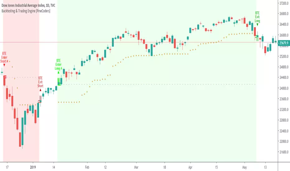
Great Expectations [LucF]Great Expectations helps traders answer the question: What is possible? It is a powerful question, yet exploration of the unknown always entails risk. A more complete set of questions better suited to traders could be:
What opportunity exists from any given point on a chart?
What portion of this opportunity can be realistically captured?
What risk will be incurred in trying to do so, and how long will it take?
Great Expectations is the result of an exploration of these questions. It is a trade simulator that generates visual and quantitative information to help strategy modelers visually identify and analyse areas of optimal expectation on charts, whether they are designing automated or discretionary strategies.
WARNING: Great Expectations is NOT an indicator that helps determine the current state of a market. It works by looking at points in the past from which the future is already known. It uses one definition of repainting extensively (i.e. it goes back in the past to print information that could not have been know at the time). Repainting understood that way is in fact almost all the indicator does! —albeit for what I hope is a noble cause. The indicator is of no use whatsoever in analyzing markets in real-time. If you do not understand what it does, please stay away!
This is an indicator—not a strategy that uses TradingView’s backtesting engine. It works by simulating trades, not unlike a backtest, but with the crucial difference that it assumes a trade (either long or short) is entered on all bars in the historic sample. It walks forward from each bar and determines possible outcomes, gathering individual trade statistics that in turn generate precious global statistics from all outcomes tested on the chart.
Great Expectations provides numbers summarizing trade results on all simulations run from the chart. Those numbers cannot be compared to backtest-produced numbers since all non-filtered bars are examined, even if an entry was taken on the bar immediately preceding the current one, which never happens in a backtest. This peculiarity does NOT invalidate Great Expectations calculations; it just entails that results be considered under a different light. Provided they are evaluated within the indicator’s context, they can be useful—sometimes even more than backtesting results, e.g. in evaluating the impact of parameter-fitting or variations in entry, exit or filtering strats.
Traders and strategy modelers are creatures of hope often suffering from blurred vision; my hope is that Great Expectations will help them appraise the validity of their setup and strat intuitions in a realistic fashion, preventing confirmation bias from obstructing perspective—and great expectations from turning into financial great deceptions.
USE CASES
You’ve identified what looks like a promising setup on other indicators. You load Great Expectations on the chart and evaluate if its high-expectation areas match locations where your setup’s conditions occur. Unless today is your lucky day, chances are the indicator will help you realize your setup is not as promising as you had hoped.
You want to get a rough estimate of the optimal trade duration for a chart and you don’t mind using the entry and exit strategies provided with the indicator. You use the trade length readouts of the indicator.
You’re experimenting with a new stop strategy and want to know how long it will keep you in trades, on average. You integrate your stop strategy in the indicator’s code and look at the average trade length it produces and the TST ratio to evaluate its performance.
You have put together your own entry and exit criteria and are looking for a filter that will help you improve backtesting results. You visually ascertain the suitability of your filter by looking at its results on the charts with great Expectations, to see if your filter is choosing its areas correctly.
You have a strategy that shows backtested trades on your chart. Great Expectations can help you evaluate how well your strategy is benefitting from high-opportunity areas while avoiding poor expectation spots.
You want more complete statistics on your set of strategies than what backtesting will provide. You use Great Expectations, knowing that it tests all bars in the sample that correspond to your criteria, as opposed to backtesting results which are limited to a subset of all possible entries.
You want to fool your friends into thinking you’ve designed the holy grail of indicators, something that identifies optimal opportunities on any chart; you show them the P&L cloud.
FEATURES
For one trade
At any given point on the chart, assuming a trade is entered there, Great Expectations shows you information specific to that trade simulation both on the chart and in the Data Window.
The chart can display:
the P & L Cloud which shows whether the trade ended profitably or not, and by how much,
the Opportunity & Risk Cloud which the maximum opportunity and risk the simulation encountered. When superimposed over the P & L cloud, you will see what I call the managed opportunity and risk, i.e the portion of maximum opportunity that was captured and the portion of the maximum risk that was incurred,
the target and if it was reached,
a background that uses a gradient to show different levels of trade length, P&L or how frequently the target was reached during simulation.
The Data Window displays more than 40 values on individual trades and global results. For any given trade you will know:
Entry/Exit levels, including slippage impact,
It’s outcome and duration,
P/L achieved,
The fraction of the maximum opportunity/risk managed by the trade.
For all trades
After going through all the possible trades on the chart, the indicator will provide you with a rare view of all outcomes expressed with the P&L cloud, which allows us to instantly see the most/least profitable areas of a chart using trade data as support, while also showing its relationship with the opportunity/risk encountered during the simulation. The difference between the two clouds is the managed opportunity and risk.
The Data Window will present you with numbers which we will go through later. Some of them are: average stop size, P/L, win rate, % opportunity managed, trade lengths for different types of trade outcomes and the TST (Target:Stop Travel) ratio.
Let’s see Great Expectations in action… and remember to open your Data Window!
INPUTS
Trade direction : You must first choose if you wish to look at long or short trades. Because of the way the indicator works and the amount of visual information on the chart, it is only practical to look at one type of trades at a time. The default is Longs.
Maximum trade Length (MaxL) : This is the maximum walk forward distance the simulator will go in analyzing outcomes from any given point in the past. It also determines the size of the dead zone among the chart’s last bars. A red background line identifies the beginning of the dead zone for which not enough bars have elapsed to analyze outcomes for the maximum trade length defined. If an ATR-based entry stop is used, that length is added to the wait time before beginning simulations, so that the first entry starts with a clean ATR value. On a sample of around 16000 bars, my tests show that the indicator runs into server errors at lengths of around 290, i.e. having completed ~4,6M simulation loop iterations. That is way too high a length anyways; 100 will usually be amply enough to ring out all the possibilities out of a simulation, and on shorter time frames, 30 can be enough. While making it unduly small will prevent simulations of expressing the market’s potential, the less you use, the faster the indicator will run. The default is 40.
Unrealized P&L base at End of Trade (EOT) : When a simulation ends and the trade is still open, we calculate unrealized P&L from an exit order executed from either the last in-trade stop on the previous bar, or the close of the last bar. You can readily see the impact of this selection on the chart, with the P&L cloud. The default is on the close.
Display : The check box besides the title does nothing.
Show target : Shows a green line displaying the trade’s target expressed as a multiple of X, i.e. the amplitude of the entry stop. I call this value “X” and use it as a unit to express profit and loss on a trade (some call it “R”). The line is highlighted for trades where the close reached the target during the trade, whether the trade ended in profit or loss. This is also where you specify the multiple of X you wish to use in calculating targets. The multiple is used even if targets are not displayed.
Show P&L Cloud : The cloud allows traders to see right away the profitable areas of the chart. The only line printed with the cloud is the “end of trade line” (EOT). The EOT line is the only way one can see the level where a trade ended on the chart (in the Data Window you can see it as the “Exit Fill” value). The EOT level for the trade determines if the trade ended in a profit or a loss. Its value represents one of the following:
- fill from order executed at close of bar where stop is breached during trade (which produces “Realized P/L”),
- simulation of a fill pseudo-fill at the user-defined EOT level (last close or stop level) if the trade runs its course through MaxL bars without getting stopped (producing Unrealized P/L).
The EOT line and the cloud fill print in green when the trade’s outcome is profitable and in red when it is not. If the trade was closed after breaching the stop, the line appears brighter.
Show Opportunity&Risk Cloud : Displays the maximum opportunity/risk that was present during the trade, i.e. the maximum and minimum prices reached.
Background Color Scheme : Allows you to choose between 3 different color schemes for the background gradients, to accommodate different types of chart background/candles. Select “None” if you don’t want a background.
Background source : Determines what value will be used to generate the different intensities of the gradient. You can choose trade length (brighter is shorter), Trade P&L (brighter is higher) or the number of times the target was reached during simulation (brighter is higher). The default is Trade Length.
Entry strat : The check box besides the title does nothing. The default strat is All bars, meaning a trade will be simulated from all bars not excluded by the filters where a MaxL bars future exists. For fun, I’ve included a pseudo-random entry strat (an indirect way of changing the seed is to vary the starting date of the simulation).
Show Filter State : Displays areas where the combination of filters you have selected are allowing entries. Filtering occurs as per your selection(s), whether the state is displayed or not. The effect of multiple selections is additive. The filters are:
1. Bar direction: Longs will only be entered if close>open and vice versa.
2. Rising Volume: Applies to both long and shorts.
3. Rising/falling MA of the length you choose over the number of bars you choose.
4. Custom indicator: You can feed your own filtering signal through this from another indicator. It must produce a signal of 1 to allow long entries and 0 to allow shorts.
Show Entry Stops :
1. Multiple of user-defined length ATR.
2. Fixed percentage.
3. Fixed value.
All entry stops are calculated using the entry fill price as a reference. The fill price is calculated from the current bar’s open, to which slippage is added if configured. This simulates the case where the strategy issued the entry signal on the previous bar for it to be executed at the next bar’s open.
The entry stop remains active until the in-trade stop becomes the more aggressive of the two stops. From then on, the entry stop will be ignored, unless a bar close breaches the in-trade stop, in which case the stop will be reset with a new entry stop and the process repeats.
Show In-trade stops : Displays in bright red the selected in-trade stop (be sure to read the note in this section about them).
1. ATR multiple: added/subtracted from the average of the two previous bars minimum/maximum of open/close.
2. A trailing stop with a deviation expressed as a multiple of entry stop (X).
3. A fixed percentage trailing stop.
Trailing stops deviations are measured from the highest/lowest high/low reached during the trade.
Note: There is a twist with the in-trade stops. It’s that for any given bar, its in-trade stop can hold multiple values, as each successive pass of the advancing simulation loops goes over it from a different entry points. What is printed is the stop from the loop that ended on that bar, which may have nothing to do with other instances of the trade’s in-trade stop for the same bar when visited from other starting points in previous simulations. There is just no practical way to print all stop values that were used for any given bar. While the printed entry stops are the actual ones used on each bar, the in-trade stops shown are merely the last instance used among many.
Include Slippage : if checked, slippage will be added/subtracted from order price to yield the fill price. Slippage is in percentage. If you choose to include slippage in the simulations, remember to adjust it by considering the liquidity of the markets and the time frame you’ll be analyzing.
Include Fees : if checked, fees will be subtracted/added to both realized an unrealized trade profits/losses. Fees are in percentage. The default fees work well for crypto markets but will need adjusting for others—especially in Forex. Remember to modify them accordingly as they can have a major impact on results. Both fees and slippage are included to remind us of their importance, even if the global numbers produced by the indicator are not representative of a real trading scenario composed of sequential trades.
Date Range filtering : the usual. Just note that the checkbox has to be selected for date filtering to activate.
DATA WINDOW
Most of the information produced by this indicator is made available in the Data Window, which you bring up by using the icon below the Watchlist and Alerts buttons at the right of the TV UI. Here’s what’s there.
Some of the information presented in the Data Window is standard trade data; other values are not so standard; e. g. the notions of managed opportunity and risk and Target:Stop Travel ratio. The interplay between all the values provided by Great Expectations is inherently complex, even for a static set of entry/filter/exit strats. During the constant updating which the habitual process of progressive refinement in building strategies that is the lot of strategy modelers entails, another level of complexity is no doubt added to the analysis of this indicator’s values. While I don’t want to sound like Wolfram presenting A New Kind of Science , I do believe that if you are a serious strategy modeler and spend the time required to get used to using all the information this indicator makes available, you may find it useful.
Trade Information
Entry Order : This is the open of the bar where simulation starts. We suppose that an entry signal was generated at the previous bar.
Entry Fill (including slip.) : The actual entry price, including slippage. This is the base price from which other values will be calculated.
Exit Order : When a stop is breached, an exit order is executed from the close of the bar that breached the stop. While there is no “In-trade stop” value included in the Data Window (other than the End of trade Stop previously discussed), this “Exit Order” value is how we can know the level where the trade was stopped during the simulation. The “Trade Length” value will then show the bar where the stop was breached.
Exit Fill (including slip.) : When the exit order is simulated, slippage is added to the order level to create the fill.
Chart: Target : This is the target calculated at the beginning of the simulation. This value also appear on the chart in teal. It is controlled by the multiple of X defined under the “Show Target” checkbox in the Inputs.
Chart: Entry Stop : This value also appears on the chart (the red dots under points where a trade was simulated). Its value is controlled by the Entry Strat chosen in the Inputs.
X (% Fill, including Fees) and X (currency) : This is the stop’s amplitude (Entry Fill – Entry Stop) + Fees. It represents the risk incurred upon entry and will be used to express P&L. We will show R expressed in both a percentage of the Entry Fill level (this value), and currency (the next value). This value represents the risk in the risk:reward ratio and is considered to be a unit of 1 so that RR can be expressed as a single value (i.e. “2” actually meaning “1:2”).
Trade Length : If trade was stopped, it’s the number of bars elapsed until then. The trade is then considered “Closed”. If the trade ends without being stopped (there is no profit-taking strat implemented, so the stop is the only exit strat), then the trade is “Open”, the length is MaxL and it will show in orange. Otherwise the value will print in green/red to reflect if the trade is winning/losing.
P&L (X) : The P&L of the trade, expressed as a multiple of X, which takes into account fees paid at entry and exit. Given our default target setting at 2 units of “X”, a trade that closes at its target will have produced a P&L of +2.0, i.e. twice the value of X (not counting fees paid at exit ). A trade that gets stopped late 50% further that the entry stop’s level will produce a P&L of -1.5X.
P&L (currency, including Fees) : same value as above, but expressed in currency.
Target first reached at bar : If price closed above the target during the trade (even if it occurs after the trade was stopped), this will show when. This value will be used in calculating our TST ratio.
Times Stop/Target reached in sim. : Includes all occurrences during the complete simulation loop.
Opportunity (X) : The highest/lowest price reached during a simulation, i.e. the maximum opportunity encountered, whether the trade was previously stopped or not, expressed as a multiple of X.
Risk (X) : The lowest/highest price reached during a simulation, i.e. the maximum risk encountered, whether the trade was previously stopped or not, expressed as a multiple of X.
Risk:Opportunity : The greater this ratio, the greater Opportunity is, compared to Risk.
Managed Opportunity (%) : The portion of Opportunity that was captured by the highest/low stop position, even if it occurred after a previous stop closed the trade.
Managed Risk (%) : The portion of risk that was protected by the lowest/highest stop position, even if it occurred after a previous stop closed the trade. When this value is greater than 100%, it means the trade’s stop is protecting more than the maximum risk, which is frequent. You will, however, never see close to those values for the Managed Opportunity value, since the stop would have to be higher than the Maximum opportunity. It is much easier to alleviate the risk than it is to lock in profits.
Managed Risk:Opportunity : The ratio of the two preceding values.
Managed Opp. vs. Risk : The Managed Opportunity minus the Managed Risk. When it is negative, which is most often is, it means your strat is protecting a greater portion of the risk than it captures opportunity.
Global Numbers
Win Rate(%) : Percentage of winning trades over all entries. Open trades are considered winning if their last stop/close (as per user selection) locks in profits.
Avg X%, Avg X (currency) : Averages of previously described values:.
Avg Profitability/Trade (APPT) : This measures expectation using: Average Profitability Per Trade = (Probability of Win × Average Win) − (Probability of Loss × Average Loss) . It quantifies the average expectation/trade, which RR alone can’t do, as the probabilities of each outcome (win/lose) must also be used to calculate expectancy. The APPT combine the RR with the win rate to yield the true expectancy of a strategy. In my usual way of expressing risk with X, APPT is the equivalent of the average P&L per trade expressed in X. An APPT of -1.5 means that we lose on average 1.5X/trade.
Equity (X), Equity (currency) : The cumulative result of all trade outcomes, expressed as a multiple of X. Multiplied by the Average X in currency, this yields the Equity in currency.
Risk:Opportunity, Managed Risk:Opportunity, Managed Opp. vs. Risk : The global values of the ones previously described.
Avg Trade Length (TL) : One of the most important values derived by going through all the simulations. Again, it is composed of either the length of stopped trades, or MaxL when the trade isn’t stopped (open). This value can help systems modelers shape the characteristics of the components they use to build their strategies.
Avg Closed Win TL and Avg Closed Lose TL : The average lengths of winning/losing trades that were stopped.
Target reached? Avg bars to Stop and Target reached? Avg bars to Target : For the trades where the target was reached at some point in the simulation, the number of bars to the first point where the stop was breached and where the target was reached, respectively. These two values are used to calculate the next value.
TST (Target:Stop Travel Ratio) : This tracks the ratio between the two preceding values (Bars to first stop/Bars to first target), but only for trades where the target was reached somewhere in the loop. A ratio of 2 means targets are reached twice as fast as stops.
The next values of this section are counts or percentages and are self-explanatory.
Chart Plots
Contains chart plots of values already describes.
NOTES
Optimization/Overfitting: There is a fine line between optimizing and overfitting. Tools like this indicator can lead unsuspecting modelers down a path of overfitting that often turns strategies into over-specialized beasts that do not perform elegantly when confronted to the real-world. Proven testing strategies like walk forward analysis will go a long way in helping modelers alleviate this risk.
Input tuning: Because the results generated by the indicator will vary with the parameters used in the active entry, filtering and exit strats, it’s important to realize that although it may be fun at first, just slapping the default settings on a chart and time frame will not yield optimal nor reliable results. While using ATR as often as possible (as I do in this indicator) is a good way to make strat parametrization adaptable, it is not a foolproof solution.
There is no data for the last MaxL bars of the chart, since not enough trade future has elapsed to run a simulation from MaxL bars back.
Modifying the code: I have tried to structure the code modularly, even if that entails a larger code base, so that you can adapt it to your needs. I’ve included a few token components in each of the placeholders designed for entry strategies, filters, entry stops and in-trade stops. This will hopefully make it easier to add your own. In the same spirit, I have also commented liberally.
You will find in the code many instances of standard trade management tasks that can be lifted to code TV strategies where, as I do in mine, you manage everything yourself and don’t rely on built-in Pine strategy functions to act on your trades.
Enjoy!
THANKS
To @scarf who showed me how plotchar() could be used to plot values without ruining scale.
To @glaz for the suggestion to include a Chandelier stop strat; I will.
To @simpelyfe for the idea of using an indicator input for the filters (if some day TV lets us use more than one, it will be useful in other modules of the indicator).
To @RicardoSantos for the random generator used in the random entry strat.
To all scripters publishing open source on TradingView; their code is the best way to learn.
To my trading buddies Irving and Bruno; who showed me way back how pro traders get it done.
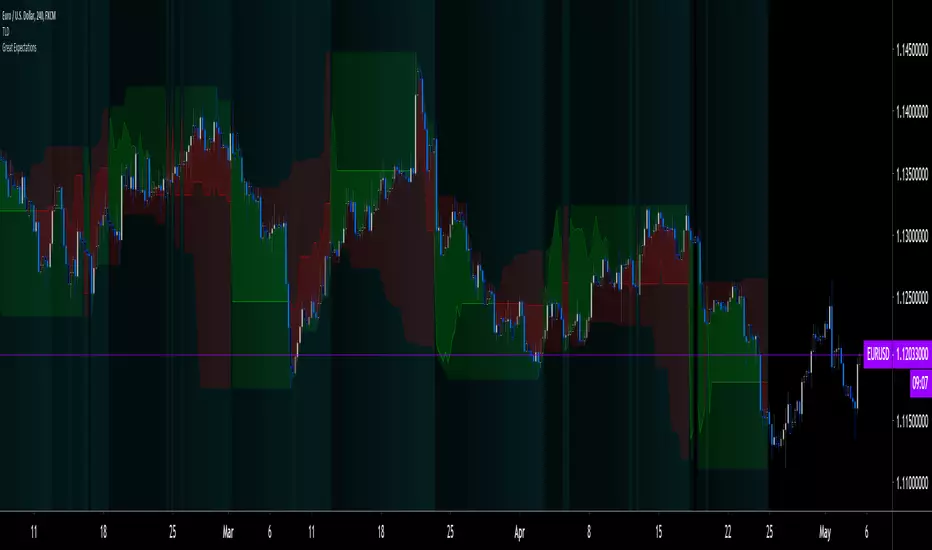
SFC Indicator_2507使用說明書 / User Manual
═══════════════════════════════════════════════════════════════════════════════
概述 / Overview
繁體中文:
SFC Indicator 是一個多功能技術分析指標,整合了布林通道、移動平均線、真實波幅均值(ATR)、箱型理論以及 Bollinger Bandit 策略。此指標專為 TradingView 平台設計,提供全面的交易信號與風險管理工具。
English:
SFC Indicator is a comprehensive technical analysis indicator that integrates Bollinger Bands, Moving Averages, Average True Range (ATR), Box Theory, and Bollinger Bandit strategy. Designed for the TradingView platform, it provides comprehensive trading signals and risk management tools.
═══════════════════════════════════════════════════════════════════════════════
主要功能 / Key Features
1. 布林通道 (Bollinger Bands)
繁體中文:
- 支援雙標準差設定 (σ1, σ2)
- 預設週期:21
- 提供上軌、中軌、下軌顯示
- 自動生成買賣信號
English:
- Supports dual standard deviation settings (σ1, σ2)
- Default period: 21
- Displays upper, middle, and lower bands
- Automatic buy/sell signal generation
2. 移動平均線 (Moving Averages)
繁體中文:
- 三條可配置的移動平均線:快線(10)、中線(20)、慢線(60)
- 支援 SMA 和 EMA 切換
- 自定義顏色設定
English:
- Three configurable moving averages: Fast (10), Medium (20), Slow (60)
- Supports SMA and EMA switching
- Customizable color settings
3. 真實波幅均值 (Average True Range - ATR)
繁體中文:
- 預設週期:14
- 支援多種平滑方式:RMA、SMA、EMA、WMA
- 動態止損計算
- 風險管理工具
English:
- Default period: 14
- Multiple smoothing methods: RMA, SMA, EMA, WMA
- Dynamic stop-loss calculation
- Risk management tool
4. 箱型理論 (Box Theory)
繁體中文:
- 自動識別價格區間
- 視覺化箱型範圍
- 突破信號提示
English:
- Automatic price range identification
- Visual box range display
- Breakout signal alerts
5. Bollinger Bandit 策略
繁體中文:
- 動態追蹤止損
- ROC (變動率) 確認
- 自適應平倉機制
English:
- Dynamic trailing stop
- ROC (Rate of Change) confirmation
- Adaptive position closing mechanism
═══════════════════════════════════════════════════════════════════════════════
參數設定 / Parameter Settings
布林通道設定 / Bollinger Bands Settings
- 布林通道均線週期 BB Period: 21 (計算週期)
- 標準差 σ1: 1 (第一標準差倍數)
- 標準差 σ2: 2 (第二標準差倍數)
移動平均線設定 / Moving Average Settings
- 快線 Fast MA: 10 (短期移動平均)
- 中線 Medium MA: 20 (中期移動平均)
- 慢線 Slow MA: 60 (長期移動平均)
- 使用 EMA: false (切換至指數移動平均)
ATR 設定 / ATR Settings
- 週期 Period: 14 (ATR 計算週期)
- 平滑方式 Smoothing: RMA (平滑算法選擇)
Bollinger Bandit 設定 / Bollinger Bandit Settings
- 布林通道週期 BB Period: 50 (Bandit 策略布林週期)
- 初始平倉均線週期 Initial Exit MA: 50 (初始止損均線週期)
- ROC 週期 ROC Period: 30 (變動率計算週期)
箱型理論設定 / Box Theory Settings
- 箱型週期 Box Period: 21 (價格區間計算週期)
═══════════════════════════════════════════════════════════════════════════════
交易信號說明 / Trading Signals
布林通道信號 / Bollinger Bands Signals
繁體中文:
- 做多信號:價格連續 X 根 K 棒低於下軌後,突破下軌向上
- 做空信號:價格連續 X 根 K 棒高於上軌後,跌破上軌向下
- 止盈目標:上軌 (Profit1) 和上 2 軌 (Profit2) 或下軌和下 2 軌
- 止損點:下 2 軌減去 ATR 值或上 2 軌加上 ATR 值
English:
- Buy Signal: Price crosses above lower band after staying below for X consecutive bars
- Sell Signal: Price crosses below upper band after staying above for X consecutive bars
- Take Profit: Upper band (Profit1) and upper 2σ band (Profit2) or lower equivalents
- Stop Loss: Lower 2σ band minus ATR value or upper 2σ band plus ATR value
Bollinger Bandit 信號 / Bollinger Bandit Signals
繁體中文:
- 做多條件:ROC > 0 且價格突破 Bandit 上軌
- 做空條件:ROC < 0 且價格跌破 Bandit 下軌
- 動態止損:使用自適應移動平均線作為追蹤止損
English:
- Buy Condition: ROC > 0 and price breaks above Bandit upper band
- Sell Condition: ROC < 0 and price breaks below Bandit lower band
- Dynamic Stop: Uses adaptive moving average as trailing stop
═══════════════════════════════════════════════════════════════════════════════
視覺元素說明 / Visual Elements
圖表元素 / Chart Elements
- 綠色三角形 ▲:做多信號 (Buy Signal)
- 紅色倒三角形 ▼:做空信號 (Sell Signal)
- 橘色線:動態止損均線 (Dynamic Stop Loss MA)
- 藍色圓點:ROC > 0 (向上動能 / Upward Momentum)
- 橘色圓點:ROC < 0 (向下動能 / Downward Momentum)
資訊面板 / Information Panel
繁體中文:
右上角顯示即時交易資訊,包含:
- 當前交易方向 (做多/做空/空手)
- 進場價格 (Entry)
- 止損價格 (Loss)
- 止盈目標 1 和 2 (Profit1, Profit2)
- Bandit 上下軌價格 (Upper, Lower)
- 動態止損線數值 (Dynamic)
English:
Top-right panel displays real-time trading information:
- Current position (Long/Short/Flat)
- Entry price
- Stop-loss price
- Take-profit targets 1 and 2
- Bandit upper/lower band prices
- Dynamic stop-loss line value
═══════════════════════════════════════════════════════════════════════════════
使用建議 / Usage Recommendations
最佳實踐 / Best Practices
繁體中文:
1. 多時間框架確認:建議在更高時間框架確認趨勢方向
2. 風險管理:嚴格遵守止損設定,建議單筆風險不超過資金的2%
3. 信號過濾:結合ROC指標過濾假信號
4. 市場環境:在趨勢明確的市場中效果較佳
5. 回測驗證:使用前請先進行充分的歷史回測
English:
1. Multi-timeframe Confirmation: Confirm trend direction on higher timeframes
2. Risk Management: Strictly follow stop-loss settings, limit single trade risk to 2% of capital
3. Signal Filtering: Use ROC indicator to filter false signals
4. Market Conditions: Works best in trending markets
5. Backtesting: Conduct thorough historical backtesting before use
適用市場 / Suitable Markets
- 股票 Stock Markets
- 外匯 Forex Markets
- 期貨 Futures Markets
- 加密貨幣 Cryptocurrency Markets
═══════════════════════════════════════════════════════════════════════════════
警示設定 / Alert Settings
繁體中文:
指標內建兩種警示功能:
- 做多信號警示:「做多訊號,來也!!!」
- 做空信號警示:「做空訊號,來也!!!」
可在 TradingView 中設定價格警示,當信號出現時自動通知。
English:
Built-in alert functions:
- Buy signal alert: "做多訊號,來也!!!" (Buy Signal Alert!)
- Sell signal alert: "做空訊號,來也!!!" (Sell Signal Alert!)
Set up price alerts in TradingView for automatic notifications when signals occur.
═══════════════════════════════════════════════════════════════════════════════
技術資訊 / Technical Information
指標作者 / Indicator Author: @lincheng_SFC
版本 / Version: Pine Script v6
授權 / License: Mozilla Public License 2.0
發布平台 / Platform: TradingView
═══════════════════════════════════════════════════════════════════════════════
免責聲明 / Disclaimer
繁體中文:
本指標僅供教育和分析用途,不構成投資建議。交易涉及風險,過往表現不代表未來結果。請在使用前進行充分測試,並根據個人風險承受能力謹慎投資。
English:
This indicator is for educational and analytical purposes only and does not constitute investment advice. Trading involves risks, and past performance does not guarantee future results. Please conduct thorough testing before use and invest carefully according to your risk tolerance.
═══════════════════════════════════════════════════════════════════════════════
聯絡資訊 / Contact Information
作者 Author: @lincheng_SFC
如有問題或建議,歡迎在TradingView上聯繫
For questions or suggestions, feel free to contact on TradingView

Machine Learning: Donchian DCA Grid Strategy [YinYangAlgorithms]This strategy uses a Machine Learning approach on the Donchian Channels with a DCA and Grid purchase/sell Strategy. Not only that, but it uses a custom Bollinger calculation to determine its Basis which is used as a mild sell location. This strategy is a pure DCA strategy in the sense that no shorts are used and theoretically it can be used in webhooks on most exchanges as it’s only using Spot Orders. The idea behind this strategy is we utilize both the Highest Highs and Lowest Lows within a Machine Learning standpoint to create Buy and Sell zones. We then fraction these zones off into pieces to create Grids. This allows us to ‘micro’ purchase as it enters these zones and likewise ‘micro’ sell as it goes up into the upper (sell) zones.
You have the option to set how many grids are used, by default we use 100 with max 1000. These grids can be ‘stacked’ together if a single bar is to go through multiple at the same time. For instance, if a bar goes through 30 grids in one bar, it will have a buy/sell power of 30x. Stacking Grid Buy and (sometimes) Sells is a very crucial part of this strategy that allows it to purchase multitudes during crashes and capitalize on sales during massive pumps.
With the grids, you’ll notice there is a middle line within the upper and lower part that makes the grid. As a Purchase Type within our Settings this is identified as ‘Middle of Zone Purchase Amount In USDT’. The middle of the grid may act as the strongest grid location (aside from maybe the bottom). Therefore there is a specific purchase amount for this Grid location.
This DCA Strategy also features two other purchase methods. Most importantly is its ‘Purchase More’ type. Essentially it will attempt to purchase when the Highest High or Lowest Low moves outside of the Outer band. For instance, the Lowest Low becomes Lower or the Higher High becomes Higher. When this happens may be a good time to buy as it is featuring a new High or Low over an extended period.
The last but not least Purchase type within this Strategy is what we call a ‘Strong Buy’. The reason for this is its verified by the following:
The outer bounds have been pushed (what causes a ‘Purchase More’)
The Price has crossed over the EMA 21
It has been verified through MACD, RSI or MACD Historical (Delta) using Regular and Hidden Divergence (Note, only 1 of these verifications is required and it can be any).
By default we don’t have Purchase Amount for ‘Strong Buy’ set, but that doesn’t mean it can’t be viable, it simply means we have only seen a few pairs where it actually proved more profitable allocating money there rather than just increasing the purchase amount for ‘Purchase More’ or ‘Grids’.
Now that you understand where we BUY, we should discuss when we SELL.
This Strategy features 3 crucial sell locations, and we will discuss each individually as they are very important.
1. ‘Sell Some At’: Here there are 4 different options, by default its set to ‘Both’ but you can change it around if you want. Your options are:
‘Both’ - You will sell some at both locations. The amount sold is the % used at ‘Sell Some %’.
‘Basis Line’ - You will sell some when the price crosses over the Basis Line. The amount sold is the % used at ‘Sell Some %’.
‘Percent’ - You will sell some when the Close is >= X% between the Lower Inner and Upper Inner Zone.
‘None’ - This simply means don’t ever Sell Some.
2. Sell Grids. Sell Grids are exactly like purchase grids and feature the same amount of grids. You also have the ability to ‘Stack Grid Sells’, which basically means if a bar moves multiple grids, it will stack the amount % wise you will sell, rather than just selling the default amount. Sell Grids use a DCA logic but for selling, which we deem may help adjust risk/reward ratio for selling, especially if there is slow but consistent bullish movement. It causes these grids to constantly push up and therefore when the close is greater than them, accrue more profit.
3. Take Profit. Take profit occurs when the close first goes above the Take Profit location (Teal Line) and then Closes below it. When Take Profit occurs, ALL POSITIONS WILL BE SOLD. What may happen is the price enters the Sell Grid, doesn’t go all the way to the top ‘Exiting it’ and then crashes back down and closes below the Take Profit. Take Profit is a strong location which generally represents a strong profit location, and that a strong momentum has changed which may cause the price to revert back to the buy grid zone.
Keep in mind, if you have (by default) ‘Only Sell If Profit’ toggled, all sell locations will only create sell orders when it is profitable to do so. Just cause it may be a good time to sell, doesn’t mean based on your DCA it is. In our opinion, only selling when it is profitable to do so is a key part of the DCA purchase strategy.
You likewise have the ability to ‘Only Buy If Lower than DCA’, which is likewise by default. These two help keep the Yin and Yang by balancing each other out where you’re only purchasing and selling when it makes logical sense too, even if that involves ignoring a signal and waiting for a better opportunity.
Tutorial:
Like most of our Strategies, we try to capitalize on lower Time Frames, generally the 15 minutes so we may find optimal entry and exit locations while still maintaining a strong correlation to trend patterns.
First off, let’s discuss examples of how this Strategy works prior to applying Machine Learning (enabled by default).
In this example above we have disabled the showing of ‘Potential Buy and Sell Signals’ so as to declutter the example. In here you can see where actual trades had gone through for both buying and selling and get an idea of how the strategy works. We also have disabled Machine Learning for this example so you can see the hard lines created by the Donchian Channel. You can also see how the Basis line ‘white line’ may act as a good location to ‘Sell Some’ and that it moves quite irregularly compared to the Donchian Channel. This is due to the fact that it is based on two custom Bollinger Bands to create the basis line.
Here we zoomed out even further and moved back a bit to where there were dense clusters of buy and sell orders. Sometimes when the price is rather volatile you’ll see it ‘Ping Pong’ back and forth between the buy and sell zones quite quickly. This may be very good for your trades and profit as a whole, especially if ‘Only Buy If Lower Than DCA’ and ‘Only Sell If Profit’ are both enabled; as these toggles will ensure you are:
Always lowering your Average when buying
Always making profit when selling
By default 8% commission is added to the Strategy as well, to simulate the cost effects of if these trades were taking place on an actual exchange.
In this example we also turned on the visuals for our ‘Purchase More’ (orange line) and ‘Take Profit’ (teal line) locations. These are crucial locations. The Purchase More makes purchases when the bottom of the grid has been moved (may dictate strong price movement has occurred and may be potential for correction). Our Take Profit may help secure profit when a momentum change is happening and all of the Sell Grids weren’t able to be used.
In the example above we’ve enabled Buy and Sell Signals so that you can see where the Take Profit and Purchase More signals have occurred. The white circle demonstrates that not all of the Position Size was sold within the Sell Grids, and therefore it was ALL CLOSED when the price closed below the Take Profit Line (Teal).
Then, when the bottom of the Donchian Channel was pushed further down due to the close (within the yellow circle), a Purchase More Signal was triggered.
When the close keeps pushing the bottom of the Buy Grid lower, it can cause multiple Purchase More Signals to occur. This is normal and also a crucial part of this strategy to help lower your DCA. Please note, the Purchase More won’t trigger a Buy if the Close is greater than the DCA and you have ‘Only Purchase If Lower Than DCA’ activated.
By turning on Machine Learning (default settings) the Buy and Sell Grid Zones are smoothed out more. It may cause it to look quite a bit different. Machine Learning although it looks much worse, may help increase the profit this Strategy can produce. Previous results DO NOT mean future results, but in this example, prior to turning on Machine Learning it had produced 37% Profit in ~5 months and with Machine Learning activated it is now up to 57% Profit in ~5 months.
Machine Learning causes the Strategy to focus less on Grids and more on Purchase More when it comes to getting its entries. However, if you likewise attempt to focus on Purchase More within non Machine Learning, the locations are different and therefore the results may not be as profitable.
PLEASE NOTE:
By default this strategy uses 1,000,000 as its initial capital. The amount it purchases in its Settings is relevant to this Initial capital. Considering this is a DCA Strategy, we only want to ‘Micro’ Buy and ‘Micro’ Sell whenever conditions are met.
Therefore, if you increase the Initial Capital, you’ll likewise want to increase the Purchase Amounts within the Settings and Vice Versa. For instance, if you wish to set the Initial Capital to 10,000, you should likewise can the amounts in the Settings to 1% of what they are to account for this.
We may change the Purchase Amounts to be based on %’s in a later update if it is requested.
We will conclude this Tutorial here, hopefully you can see how a DCA Grid Purchase Model applied to Machine Learning Donchian Channels may be useful for making strategic purchases in low and high zones.
Settings:
Display Data:
Show Potential Buy Locations: These locations are where 'Potentially' orders can be placed. Placement of orders is dependant on if you have 'Only Buy If Lower Than DCA' toggled and the Price is lower than DCA. It also is effected by if you actually have any money left to purchase with; you can't buy if you have no money left!
Show Potential Sell Locations: These locations are where 'Potentially' orders will be sold. If 'Only Sell If Profit' is toggled, the sell will only happen if you'll make profit from it!
Show Grid Locations: Displaying won't affect your trades but it can be useful to see where trades will be placed, as well as which have gone through and which are left to be purchased. Max 100 Grids, but visuals will only be shown if its 20 or less.
Purchase Settings:
Only Buy if its lower than DCA: Generally speaking, we want to lower our Average, and therefore it makes sense to only buy when the close is lower than our current DCA and a Purchase Condition is met.
Compound Purchases: Compounding Purchases means reinvesting profit back into your trades right away. It drastically increases profits, but it also increases risk too. It will adjust your Purchase Amounts for the Purchase Type you have set at the same % rate of strategy initial_capital to the amounts you have set.
Adjust Purchase Amount Ratio to Maintain Risk level: By adjusting purchase levels we generally help maintain a safe risk level. Basically we generally want to reserve X amount of % for each purchase type being used and relocate money when there is too much in one type. This helps balance out purchase amounts and ensure the types selected have a correct ratio to ensure they can place the right amount of orders.
Stack Grid Buys: Stacking Buy Grids is when the Close crosses multiple Buy Grids within the same bar. Should we still only purchase the value of 1 Buy Grid OR stack the grid buys based on how many buy grids it went through.
Purchase Type: Where do you want to make Purchases? We recommend lowering your risk by combining All purchase types, but you may also customize your trading strategy however you wish.
Strong Buy Purchase Amount In USDT: How much do you want to purchase when the 'Strong Buy' signal appears? This signal only occurs after it has at least entered the Buy Zone and there have been other verifications saying it's now a good time to buy. Our Strong Buy Signal is a very strong indicator that a large price movement towards the Sell Zone will likely occur. It almost always results in it leaving the Buy Zone and usually will go to at least the White Basis line where you can 'Sell Some'.
Buy More Purchase Amount In USDT: How much should you purchase when the 'Purchase More' signal appears? This 'Purchase More' signal occurs when the lowest level of the Buy Zone moves lower. This is a great time to buy as you're buying the dip and generally there is a correction that will allow you to 'Sell Some' for some profit.
Amount of Grid Buy and Sells: How many Grid Purchases do you want to make? We recommend having it at the max of 10, as it will essentially get you a better Average Purchase Price, but you may adjust it to whatever you wish. This amount also only matters if your Purchase Type above incorporates Grid Purchases. Max 100 Grids, but visuals will only be shown if it's 20 or less.
Each Grid Purchase Amount In USDT: How much should you purchase after closing under a grid location? Keep in mind, if you have 10 grids and it goes through each, it will be this amount * 10. Grid purchasing is a great way to get a good entry, lower risk and also lower your average.
Middle Of Zone Purchase Amount In USDT: The Middle Of Zone is the strongest grid location within the Buy Zone. This is why we have a unique Purchase Amount for this Grid specifically. Please note you need to have 'Middle of Zone is a Grid' enabled for this Purchase Amount to be used.
Sell:
Only Sell if its Profit: There is a chance that during a dump, all your grid buys when through, and a few Purchase More Signals have appeared. You likely got a good entry. A Strong Buy may also appear before it starts to pump to the Sell Zone. The issue that may occur is your Average Purchase Price is greater than the 'Sell Some' price and/or the Grids in the Sell Zone and/or the Strong Sell Signal. When this happens, you can either take a loss and sell it, or you can hold on to it and wait for more purchase signals to therefore lower your average more so you can take profit at the next sell location. Please backtest this yourself within our YinYang Purchase Strategy on the pair and timeframe you are wanting to trade on. Please also note, that previous results will not always reflect future results. Please assess the risk yourself. Don't trade what you can't afford to lose. Sometimes it is better to strategically take a loss and continue on making profit than to stay in a bad trade for a long period of time.
Stack Grid Sells: Stacking Sell Grids is when the Close crosses multiple Sell Grids within the same bar. Should we still only sell the value of 1 Sell Grid OR stack the grid sells based on how many sell grids it went through.
Stop Loss Type: This is when the Close has pushed the Bottom of the Buy Grid More. Do we Stop Loss or Purchase More?? By default we recommend you stay true to the DCA part of this strategy by Purchasing More, but this is up to you.
Sell Some At: Where if selected should we 'Sell Some', this may be an important way to sell a little bit at a good time before the price may correct. Also, we don't want to sell too much incase it doesn't correct though, so its a 'Sell Some' location. Basis Line refers to our Moving Basis Line created from 2 Bollinger Bands and Percent refers to a Percent difference between the Lower Inner and Upper Inner bands.
Sell Some At Percent Amount: This refers to how much % between the Lower Inner and Upper Inner bands we should well at if we chose to 'Sell Some'.
Sell Some Min %: This refers to the Minimum amount between the Lower Inner band and Close that qualifies a 'Sell Some'. This acts as a failsafe so we don't 'Sell Some' for too little.
Sell % At Strong Sell Signal: How much do we sell at the 'Strong Sell' Signal? It may act as a strong location to sell, but likewise Grid Sells could be better.
Grid and Donchian Settings:
Donchian Channel Length: How far back are we looking back to determine our Donchian Channel.
Extra Outer Buy Width %: How much extra should we push the Outer Buy (Low) Width by?
Extra Inner Buy Width %: How much extra should we push the Inner Buy (Low) Width by?
Extra Inner Sell Width %: How much extra should we push the Inner Sell (High) Width by?
Extra Outer Sell Width %: How much extra should we push the Outer Sell (High) Width by?
Machine Learning:
Rationalized Source Type: Donchians usually use High/Low. What Source is our Rationalized Source using?
Machine Learning Type: Are we using a Simple ML Average, KNN Mean Average, KNN Exponential Average or None?
Machine Learning Length: How far back is our Machine Learning going to keep data for.
k-Nearest Neighbour (KNN) Length: How many k-Nearest Neighbours will we account for?
Fast ML Data Length: What is our Fast ML Length?? This is used with our Slow Length to create our KNN Distance.
Slow ML Data Length: What is our Slow ML Length?? This is used with our Fast Length to create our KNN Distance.
If you have any questions, comments, ideas or concerns please don't hesitate to contact us.
HAPPY TRADING!
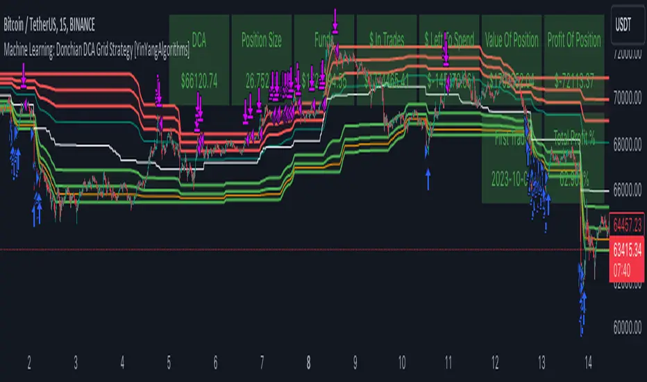
GKD-C Adaptive-Lookback Phase Change Index [Loxx]Giga Kaleidoscope GKD-C Adaptive-Lookback Phase Change Index is a Confirmation module included in Loxx's "Giga Kaleidoscope Modularized Trading System".
█ GKD-C Adaptive-Lookback Phase Change Index
What is the Phase Change Index?
The Phase Change Index (PCI) is a technical indicator that has gained popularity among traders in recent years. It is used to identify market phases and make profitable trades based on momentum and price data. The PCI was developed by M.H. Pee and first introduced in the Stocks & Commodities magazine in 2004.
The PCI is calculated using the 35-day momentum and the 35-day price channel index (PCI). The momentum is the difference between the current day's close and the close 35 days ago, while the PCI measures the distance between the highest high and lowest low over a period of 35 days. By combining these two indicators, traders can identify six possible market phases, each with its own trading strategy.
The formula for calculating the Phase Change Index (PCI) is as follows:
PCI = 100 * (C - L) / (H - L)
Where:
- C is the closing price of the current day
- L is the lowest low over a period of 35 days
- H is the highest high over a period of 35 days
The formula for calculating momentum is as follows:
Momentum = C - Cn
Where:
- C is the closing price of the current day
- Cn is the closing price n days ago, where n = 35 in this case.
The first two phases are characterized by negative momentum, with phase one having a low PCI value (less than 20) and phase two having a high PCI value (greater than 80). In these phases, traders should enter short positions. The next two phases have positive momentum, with phase three having a low PCI value and phase four having a high PCI value. In these phases, traders should enter long positions.
The final two phases are characterized by neutral momentum, with phase five having a low PCI value and phase six having a high PCI value. In these phases, traders should maintain their previous positions until there is a clear signal to enter or exit.
Traders can also use other technical indicators in conjunction with the PCI to confirm signals or filter out false signals. For example, some traders use moving averages or trendlines to confirm trend direction before entering a trade based on the PCI.
In conclusion, the Phase Change Index is a powerful technical indicator that can help traders identify market phases and make profitable trades. By combining momentum and price data, traders can enter long or short positions based on the six possible market phases. Backtesting results have shown that the PCI is robust across parameters, markets, and years. However, it is important to use proper risk management and not rely solely on past profitability when making trading decisions.
What is the Jurik Filter?
The Jurik Filter is a technical analysis tool that is used to filter out market noise and identify trends in financial markets. It was developed by Mark Jurik in the 1990s and is based on a non-linear smoothing algorithm that provides a more accurate representation of price movements.
Traditional moving averages, such as the Simple Moving Average ( SMA ) or Exponential Moving Average ( EMA ), are linear filters that produce a lag between price and the moving average line. This can cause false signals during periods of market volatility , which can result in losses for traders and investors.
The Jurik Filter is designed to address this issue by incorporating a damping factor into the smoothing algorithm. This damping factor adjusts the filter's responsiveness to the changes in price, allowing it to filter out market noise without overshooting price peaks and valleys.
The Jurik Filter is calculated using a mathematical formula that takes into account the current and past prices of an asset, as well as the volatility of the market. This formula incorporates the damping factor and produces a smoother price curve than traditional moving average filters.
One of the advantages of the Jurik Filter is its ability to adjust to changing market conditions. The damping factor can be adjusted to suit different securities and time frames, making it a versatile tool for traders and investors.
Traders and investors often use the Jurik Filter in conjunction with other technical analysis tools, such as the MACD or RSI , to confirm or complement their trading strategies. By filtering out market noise and identifying trends in the financial markets, the Jurik Filter can help improve the accuracy of trading signals and reduce the risks of false signals during periods of market volatility .
Overall, the Jurik Filter is a powerful technical analysis tool that can help traders and investors make more informed decisions about buying and selling securities. By providing a smoother price curve and reducing false signals, it can help improve trading performance and reduce risk in volatile markets.
What is the Adaptive Lookback Period?
The adaptive lookback period is a technique used in technical analysis to adjust the period of an indicator based on changes in market conditions. This technique is particularly useful in volatile or rapidly changing markets where a fixed period may not be optimal for detecting trends or signals.
The concept of the adaptive lookback period is relatively simple. By adjusting the lookback period based on changes in market conditions, traders can more accurately identify trends and signals. This can help traders to enter and exit trades at the right time and improve the profitability of their trading strategies.
The adaptive lookback period works by identifying potential swing points in the market. Once these points are identified, the lookback period is calculated based on the number of swings and a speed parameter. The swing count parameter determines the number of swings that must occur before the lookback period is adjusted. The speed parameter controls the rate at which the lookback period is adjusted, with higher values indicating a more rapid adjustment.
The adaptive lookback period can be applied to a wide range of technical indicators, including moving averages, oscillators, and trendlines. By adjusting the period of these indicators based on changes in market conditions, traders can reduce the impact of noise and false signals, leading to more profitable trades.
In summary, the adaptive lookback period is a powerful technique for traders and analysts looking to optimize their technical indicators. By adjusting the period based on changes in market conditions, traders can more accurately identify trends and signals, leading to more profitable trades. While there are various ways to implement the adaptive lookback period, the basic concept remains the same, and traders can adapt and customize the technique to suit their individual needs and trading styles.
What is the Adaptive-Lookback Phase Change Index?
The combination of adaptive lookback and Jurik filtering is an effective technique used in technical analysis to filter out market noise and improve the accuracy of trading signals. When applied to the Phase Change Index (PCI) indicator, the adaptive lookback period can be used to adjust the period of the indicator based on changes in market conditions. Jurik filtering can then be used to filter out market noise and improve the accuracy of the signals produced by the PCI indicator.
The adaptive lookback period is particularly useful in volatile or rapidly changing markets where a fixed period may not be optimal for detecting trends or signals. By adjusting the lookback period based on changes in market conditions, traders can more accurately identify trends and signals, leading to more profitable trades.
Jurik filtering is a more advanced filtering technique that uses a combination of smoothing and phase shift to produce a more accurate signal. This technique is particularly useful in filtering out market noise and improving the accuracy of trading signals. Jurik filtering can be applied to various indicators, including moving averages, oscillators, and trendlines.
Overall, the combination of adaptive lookback and Jurik filtering is a powerful technique used in technical analysis to filter out market noise and improve the accuracy of trading signals. When applied to the Phase Change Index (PCI) indicator, this technique is particularly effective in identifying trend changes and producing more accurate signals for entry and exit points in trading strategies.
Keep in mind, this is an inverse indicator meaning that above the middle-line/signal is short, below is long.
Additional Features
This indicator allows you to select from 33 source types. They are as follows:
Close
Open
High
Low
Median
Typical
Weighted
Average
Average Median Body
Trend Biased
Trend Biased (Extreme)
HA Close
HA Open
HA High
HA Low
HA Median
HA Typical
HA Weighted
HA Average
HA Average Median Body
HA Trend Biased
HA Trend Biased (Extreme)
HAB Close
HAB Open
HAB High
HAB Low
HAB Median
HAB Typical
HAB Weighted
HAB Average
HAB Average Median Body
HAB Trend Biased
HAB Trend Biased (Extreme)
What are Heiken Ashi "better" candles?
Heiken Ashi "better" candles are a modified version of the standard Heiken Ashi candles, which are a popular charting technique used in technical analysis. Heiken Ashi candles help traders identify trends and potential reversal points by smoothing out price data and reducing market noise. The "better formula" was proposed by Sebastian Schmidt in an article published by BNP Paribas in Warrants & Zertifikate, a German magazine, in August 2004. The aim of this formula is to further improve the smoothing of the Heiken Ashi chart and enhance its effectiveness in identifying trends and reversals.
Standard Heiken Ashi candles are calculated using the following formulas:
Heiken Ashi Close = (Open + High + Low + Close) / 4
Heiken Ashi Open = (Previous Heiken Ashi Open + Previous Heiken Ashi Close) / 2
Heiken Ashi High = Max (High, Heiken Ashi Open, Heiken Ashi Close)
Heiken Ashi Low = Min (Low, Heiken Ashi Open, Heiken Ashi Close)
The "better formula" modifies the standard Heiken Ashi calculation by incorporating additional smoothing, which can help reduce noise and make it easier to identify trends and reversals. The modified formulas for Heiken Ashi "better" candles are as follows:
Better Heiken Ashi Close = (Open + High + Low + Close) / 4
Better Heiken Ashi Open = (Previous Better Heiken Ashi Open + Previous Better Heiken Ashi Close) / 2
Better Heiken Ashi High = Max (High, Better Heiken Ashi Open, Better Heiken Ashi Close)
Better Heiken Ashi Low = Min (Low, Better Heiken Ashi Open, Better Heiken Ashi Close)
Smoothing Factor = 2 / (N + 1), where N is the chosen period for smoothing
Smoothed Better Heiken Ashi Open = (Better Heiken Ashi Open * Smoothing Factor) + (Previous Smoothed Better Heiken Ashi Open * (1 - Smoothing Factor))
Smoothed Better Heiken Ashi Close = (Better Heiken Ashi Close * Smoothing Factor) + (Previous Smoothed Better Heiken Ashi Close * (1 - Smoothing Factor))
The smoothed Better Heiken Ashi Open and Close values are then used to calculate the smoothed Better Heiken Ashi High and Low values, resulting in "better" candles that provide a clearer representation of the market trend and potential reversal points.
It's important to note that, like any other technical analysis tool, Heiken Ashi "better" candles are not foolproof and should be used in conjunction with other indicators and analysis techniques to make well-informed trading decisions.
Heiken Ashi "better" candles, as mentioned previously, provide a clearer representation of market trends and potential reversal points by reducing noise and smoothing out price data. When using these candles in conjunction with other technical analysis tools and indicators, traders can gain valuable insights into market behavior and make more informed decisions.
To effectively use Heiken Ashi "better" candles in your trading strategy, consider the following tips:
Trend Identification: Heiken Ashi "better" candles can help you identify the prevailing trend in the market. When the majority of the candles are green (or another color, depending on your chart settings) and there are no or few lower wicks, it may indicate a strong uptrend. Conversely, when the majority of the candles are red (or another color) and there are no or few upper wicks, it may signal a strong downtrend.
Trend Reversals: Look for potential trend reversals when a change in the color of the candles occurs, especially when accompanied by longer wicks. For example, if a green candle with a long lower wick is followed by a red candle, it could indicate a bearish reversal. Similarly, a red candle with a long upper wick followed by a green candle may suggest a bullish reversal.
Support and Resistance: You can use Heiken Ashi "better" candles to identify potential support and resistance levels. When the candles are consistently moving in one direction and then suddenly change color with longer wicks, it could indicate the presence of a support or resistance level.
Stop-Loss and Take-Profit: Using Heiken Ashi "better" candles can help you manage risk by determining optimal stop-loss and take-profit levels. For instance, you can place your stop-loss below the low of the most recent green candle in an uptrend or above the high of the most recent red candle in a downtrend.
Confirming Signals: Heiken Ashi "better" candles should be used in conjunction with other technical indicators, such as moving averages, oscillators, or chart patterns, to confirm signals and improve the accuracy of your analysis.
In this implementation, you have the choice of AMA, KAMA, or T3 smoothing. These are as follows:
Kaufman Adaptive Moving Average (KAMA)
The Kaufman Adaptive Moving Average (KAMA) is a type of adaptive moving average used in technical analysis to smooth out price fluctuations and identify trends. The KAMA adjusts its smoothing factor based on the market's volatility, making it more responsive in volatile markets and smoother in calm markets. The KAMA is calculated using three different efficiency ratios that determine the appropriate smoothing factor for the current market conditions. These ratios are based on the noise level of the market, the speed at which the market is moving, and the length of the moving average. The KAMA is a popular choice among traders who prefer to use adaptive indicators to identify trends and potential reversals.
Adaptive Moving Average
The Adaptive Moving Average (AMA) is a type of moving average that adjusts its sensitivity to price movements based on market conditions. It uses a ratio between the current price and the highest and lowest prices over a certain lookback period to determine its level of smoothing. The AMA can help reduce lag and increase responsiveness to changes in trend direction, making it useful for traders who want to follow trends while avoiding false signals. The AMA is calculated by multiplying a smoothing constant with the difference between the current price and the previous AMA value, then adding the result to the previous AMA value.
T3
The T3 moving average is a type of technical indicator used in financial analysis to identify trends in price movements. It is similar to the Exponential Moving Average (EMA) and the Double Exponential Moving Average (DEMA), but uses a different smoothing algorithm.
The T3 moving average is calculated using a series of exponential moving averages that are designed to filter out noise and smooth the data. The resulting smoothed data is then weighted with a non-linear function to produce a final output that is more responsive to changes in trend direction.
The T3 moving average can be customized by adjusting the length of the moving average, as well as the weighting function used to smooth the data. It is commonly used in conjunction with other technical indicators as part of a larger trading strategy.
█ Giga Kaleidoscope Modularized Trading System
Core components of an NNFX algorithmic trading strategy
The NNFX algorithm is built on the principles of trend, momentum, and volatility. There are six core components in the NNFX trading algorithm:
1. Volatility - price volatility; e.g., Average True Range, True Range Double, Close-to-Close, etc.
2. Baseline - a moving average to identify price trend
3. Confirmation 1 - a technical indicator used to identify trends
4. Confirmation 2 - a technical indicator used to identify trends
5. Continuation - a technical indicator used to identify trends
6. Volatility/Volume - a technical indicator used to identify volatility/volume breakouts/breakdown
7. Exit - a technical indicator used to determine when a trend is exhausted
What is Volatility in the NNFX trading system?
In the NNFX (No Nonsense Forex) trading system, ATR (Average True Range) is typically used to measure the volatility of an asset. It is used as a part of the system to help determine the appropriate stop loss and take profit levels for a trade. ATR is calculated by taking the average of the true range values over a specified period.
True range is calculated as the maximum of the following values:
-Current high minus the current low
-Absolute value of the current high minus the previous close
-Absolute value of the current low minus the previous close
ATR is a dynamic indicator that changes with changes in volatility. As volatility increases, the value of ATR increases, and as volatility decreases, the value of ATR decreases. By using ATR in NNFX system, traders can adjust their stop loss and take profit levels according to the volatility of the asset being traded. This helps to ensure that the trade is given enough room to move, while also minimizing potential losses.
Other types of volatility include True Range Double (TRD), Close-to-Close, and Garman-Klass
What is a Baseline indicator?
The baseline is essentially a moving average, and is used to determine the overall direction of the market.
The baseline in the NNFX system is used to filter out trades that are not in line with the long-term trend of the market. The baseline is plotted on the chart along with other indicators, such as the Moving Average (MA), the Relative Strength Index (RSI), and the Average True Range (ATR).
Trades are only taken when the price is in the same direction as the baseline. For example, if the baseline is sloping upwards, only long trades are taken, and if the baseline is sloping downwards, only short trades are taken. This approach helps to ensure that trades are in line with the overall trend of the market, and reduces the risk of entering trades that are likely to fail.
By using a baseline in the NNFX system, traders can have a clear reference point for determining the overall trend of the market, and can make more informed trading decisions. The baseline helps to filter out noise and false signals, and ensures that trades are taken in the direction of the long-term trend.
What is a Confirmation indicator?
Confirmation indicators are technical indicators that are used to confirm the signals generated by primary indicators. Primary indicators are the core indicators used in the NNFX system, such as the Average True Range (ATR), the Moving Average (MA), and the Relative Strength Index (RSI).
The purpose of the confirmation indicators is to reduce false signals and improve the accuracy of the trading system. They are designed to confirm the signals generated by the primary indicators by providing additional information about the strength and direction of the trend.
Some examples of confirmation indicators that may be used in the NNFX system include the Bollinger Bands, the MACD (Moving Average Convergence Divergence), and the MACD Oscillator. These indicators can provide information about the volatility, momentum, and trend strength of the market, and can be used to confirm the signals generated by the primary indicators.
In the NNFX system, confirmation indicators are used in combination with primary indicators and other filters to create a trading system that is robust and reliable. By using multiple indicators to confirm trading signals, the system aims to reduce the risk of false signals and improve the overall profitability of the trades.
What is a Continuation indicator?
In the NNFX (No Nonsense Forex) trading system, a continuation indicator is a technical indicator that is used to confirm a current trend and predict that the trend is likely to continue in the same direction. A continuation indicator is typically used in conjunction with other indicators in the system, such as a baseline indicator, to provide a comprehensive trading strategy.
What is a Volatility/Volume indicator?
Volume indicators, such as the On Balance Volume (OBV), the Chaikin Money Flow (CMF), or the Volume Price Trend (VPT), are used to measure the amount of buying and selling activity in a market. They are based on the trading volume of the market, and can provide information about the strength of the trend. In the NNFX system, volume indicators are used to confirm trading signals generated by the Moving Average and the Relative Strength Index. Volatility indicators include Average Direction Index, Waddah Attar, and Volatility Ratio. In the NNFX trading system, volatility is a proxy for volume and vice versa.
By using volume indicators as confirmation tools, the NNFX trading system aims to reduce the risk of false signals and improve the overall profitability of trades. These indicators can provide additional information about the market that is not captured by the primary indicators, and can help traders to make more informed trading decisions. In addition, volume indicators can be used to identify potential changes in market trends and to confirm the strength of price movements.
What is an Exit indicator?
The exit indicator is used in conjunction with other indicators in the system, such as the Moving Average (MA), the Relative Strength Index (RSI), and the Average True Range (ATR), to provide a comprehensive trading strategy.
The exit indicator in the NNFX system can be any technical indicator that is deemed effective at identifying optimal exit points. Examples of exit indicators that are commonly used include the Parabolic SAR, the Average Directional Index (ADX), and the Chandelier Exit.
The purpose of the exit indicator is to identify when a trend is likely to reverse or when the market conditions have changed, signaling the need to exit a trade. By using an exit indicator, traders can manage their risk and prevent significant losses.
In the NNFX system, the exit indicator is used in conjunction with a stop loss and a take profit order to maximize profits and minimize losses. The stop loss order is used to limit the amount of loss that can be incurred if the trade goes against the trader, while the take profit order is used to lock in profits when the trade is moving in the trader's favor.
Overall, the use of an exit indicator in the NNFX trading system is an important component of a comprehensive trading strategy. It allows traders to manage their risk effectively and improve the profitability of their trades by exiting at the right time.
How does Loxx's GKD (Giga Kaleidoscope Modularized Trading System) implement the NNFX algorithm outlined above?
Loxx's GKD v1.0 system has five types of modules (indicators/strategies). These modules are:
1. GKD-BT - Backtesting module (Volatility, Number 1 in the NNFX algorithm)
2. GKD-B - Baseline module (Baseline and Volatility/Volume, Numbers 1 and 2 in the NNFX algorithm)
3. GKD-C - Confirmation 1/2 and Continuation module (Confirmation 1/2 and Continuation, Numbers 3, 4, and 5 in the NNFX algorithm)
4. GKD-V - Volatility/Volume module (Confirmation 1/2, Number 6 in the NNFX algorithm)
5. GKD-E - Exit module (Exit, Number 7 in the NNFX algorithm)
(additional module types will added in future releases)
Each module interacts with every module by passing data between modules. Data is passed between each module as described below:
GKD-B => GKD-V => GKD-C(1) => GKD-C(2) => GKD-C(Continuation) => GKD-E => GKD-BT
That is, the Baseline indicator passes its data to Volatility/Volume. The Volatility/Volume indicator passes its values to the Confirmation 1 indicator. The Confirmation 1 indicator passes its values to the Confirmation 2 indicator. The Confirmation 2 indicator passes its values to the Continuation indicator. The Continuation indicator passes its values to the Exit indicator, and finally, the Exit indicator passes its values to the Backtest strategy.
This chaining of indicators requires that each module conform to Loxx's GKD protocol, therefore allowing for the testing of every possible combination of technical indicators that make up the six components of the NNFX algorithm.
What does the application of the GKD trading system look like?
Example trading system:
Backtest: Strategy with 1-3 take profits, trailing stop loss, multiple types of PnL volatility, and 2 backtesting styles
Baseline: Hull Moving Average
Volatility/Volume: Hurst Exponent
Confirmation 1: Adaptive-Lookback Phase Change Index as shown on the chart above
Confirmation 2: Williams Percent Range
Continuation: Fisher Transform
Exit: Rex Oscillator
Each GKD indicator is denoted with a module identifier of either: GKD-BT, GKD-B, GKD-C, GKD-V, or GKD-E. This allows traders to understand to which module each indicator belongs and where each indicator fits into the GKD protocol chain.
Giga Kaleidoscope Modularized Trading System Signals (based on the NNFX algorithm)
Standard Entry
1. GKD-C Confirmation 1 Signal
2. GKD-B Baseline agrees
3. Price is within a range of 0.2x Volatility and 1.0x Volatility of the Goldie Locks Mean
4. GKD-C Confirmation 2 agrees
5. GKD-V Volatility/Volume agrees
Baseline Entry
1. GKD-B Baseline signal
2. GKD-C Confirmation 1 agrees
3. Price is within a range of 0.2x Volatility and 1.0x Volatility of the Goldie Locks Mean
4. GKD-C Confirmation 2 agrees
5. GKD-V Volatility/Volume agrees
6. GKD-C Confirmation 1 signal was less than 7 candles prior
Volatility/Volume Entry
1. GKD-V Volatility/Volume signal
2. GKD-C Confirmation 1 agrees
3. Price is within a range of 0.2x Volatility and 1.0x Volatility of the Goldie Locks Mean
4. GKD-C Confirmation 2 agrees
5. GKD-B Baseline agrees
6. GKD-C Confirmation 1 signal was less than 7 candles prior
Continuation Entry
1. Standard Entry, Baseline Entry, or Pullback; entry triggered previously
2. GKD-B Baseline hasn't crossed since entry signal trigger
3. GKD-C Confirmation Continuation Indicator signals
4. GKD-C Confirmation 1 agrees
5. GKD-B Baseline agrees
6. GKD-C Confirmation 2 agrees
1-Candle Rule Standard Entry
1. GKD-C Confirmation 1 signal
2. GKD-B Baseline agrees
3. Price is within a range of 0.2x Volatility and 1.0x Volatility of the Goldie Locks Mean
Next Candle:
1. Price retraced (Long: close < close or Short: close > close )
2. GKD-B Baseline agrees
3. GKD-C Confirmation 1 agrees
4. GKD-C Confirmation 2 agrees
5. GKD-V Volatility/Volume agrees
1-Candle Rule Baseline Entry
1. GKD-B Baseline signal
2. GKD-C Confirmation 1 agrees
3. Price is within a range of 0.2x Volatility and 1.0x Volatility of the Goldie Locks Mean
4. GKD-C Confirmation 1 signal was less than 7 candles prior
Next Candle:
1. Price retraced (Long: close < close or Short: close > close )
2. GKD-B Baseline agrees
3. GKD-C Confirmation 1 agrees
4. GKD-C Confirmation 2 agrees
5. GKD-V Volatility/Volume Agrees
1-Candle Rule Volatility/Volume Entry
1. GKD-V Volatility/Volume signal
2. GKD-C Confirmation 1 agrees
3. Price is within a range of 0.2x Volatility and 1.0x Volatility of the Goldie Locks Mean
4. GKD-C Confirmation 1 signal was less than 7 candles prior
Next Candle:
1. Price retraced (Long: close < close or Short: close > close)
2. GKD-B Volatility/Volume agrees
3. GKD-C Confirmation 1 agrees
4. GKD-C Confirmation 2 agrees
5. GKD-B Baseline agrees
PullBack Entry
1. GKD-B Baseline signal
2. GKD-C Confirmation 1 agrees
3. Price is beyond 1.0x Volatility of Baseline
Next Candle:
1. Price is within a range of 0.2x Volatility and 1.0x Volatility of the Goldie Locks Mean
2. GKD-C Confirmation 1 agrees
3. GKD-C Confirmation 2 agrees
4. GKD-V Volatility/Volume Agrees
]█ Setting up the GKD
The GKD system involves chaining indicators together. These are the steps to set this up.
Use a GKD-C indicator alone on a chart
1. Inside the GKD-C indicator, change the "Confirmation Type" setting to "Solo Confirmation Simple"
Use a GKD-V indicator alone on a chart
**nothing, it's already useable on the chart without any settings changes
Use a GKD-B indicator alone on a chart
**nothing, it's already useable on the chart without any settings changes
Baseline (Baseline, Backtest)
1. Import the GKD-B Baseline into the GKD-BT Backtest: "Input into Volatility/Volume or Backtest (Baseline testing)"
2. Inside the GKD-BT Backtest, change the setting "Backtest Special" to "Baseline"
Volatility/Volume (Volatility/Volume, Backte st)
1. Inside the GKD-V indicator, change the "Testing Type" setting to "Solo"
2. Inside the GKD-V indicator, change the "Signal Type" setting to "Crossing" (neither traditional nor both can be backtested)
3. Import the GKD-V indicator into the GKD-BT Backtest: "Input into C1 or Backtest"
4. Inside the GKD-BT Backtest, change the setting "Backtest Special" to "Volatility/Volume"
5. Inside the GKD-BT Backtest, a) change the setting "Backtest Type" to "Trading" if using a directional GKD-V indicator; or, b) change the setting "Backtest Type" to "Full" if using a directional or non-directional GKD-V indicator (non-directional GKD-V can only test Longs and Shorts separately)
6. If "Backtest Type" is set to "Full": Inside the GKD-BT Backtest, change the setting "Backtest Side" to "Long" or "Short
7. If "Backtest Type" is set to "Full": To allow the system to open multiple orders at one time so you test all Longs or Shorts, open the GKD-BT Backtest, click the tab "Properties" and then insert a value of something like 10 orders into the "Pyramiding" settings. This will allow 10 orders to be opened at one time which should be enough to catch all possible Longs or Shorts.
Solo Confirmation Simple (Confirmation, Backtest)
1. Inside the GKD-C indicator, change the "Confirmation Type" setting to "Solo Confirmation Simple"
1. Import the GKD-C indicator into the GKD-BT Backtest: "Input into Backtest"
2. Inside the GKD-BT Backtest, change the setting "Backtest Special" to "Solo Confirmation Simple"
Solo Confirmation Complex without Exits (Baseline, Volatility/Volume, Confirmation, Backtest)
1. Inside the GKD-V indicator, change the "Testing Type" setting to "Chained"
2. Import the GKD-B Baseline into the GKD-V indicator: "Input into Volatility/Volume or Backtest (Baseline testing)"
3. Inside the GKD-C indicator, change the "Confirmation Type" setting to "Solo Confirmation Complex"
4. Import the GKD-V indicator into the GKD-C indicator: "Input into C1 or Backtest"
5. Inside the GKD-BT Backtest, change the setting "Backtest Special" to "GKD Full wo/ Exits"
6. Import the GKD-C into the GKD-BT Backtest: "Input into Exit or Backtest"
Solo Confirmation Complex with Exits (Baseline, Volatility/Volume, Confirmation, Exit, Backtest)
1. Inside the GKD-V indicator, change the "Testing Type" setting to "Chained"
2. Import the GKD-B Baseline into the GKD-V indicator: "Input into Volatility/Volume or Backtest (Baseline testing)"
3. Inside the GKD-C indicator, change the "Confirmation Type" setting to "Solo Confirmation Complex"
4. Import the GKD-V indicator into the GKD-C indicator: "Input into C1 or Backtest"
5. Import the GKD-C indicator into the GKD-E indicator: "Input into Exit"
6. Inside the GKD-BT Backtest, change the setting "Backtest Special" to "GKD Full w/ Exits"
7. Import the GKD-E into the GKD-BT Backtest: "Input into Backtest"
Full GKD without Exits (Baseline, Volatility/Volume, Confirmation 1, Confirmation 2, Continuation, Backtest)
1. Inside the GKD-V indicator, change the "Testing Type" setting to "Chained"
2. Import the GKD-B Baseline into the GKD-V indicator: "Input into Volatility/Volume or Backtest (Baseline testing)"
3. Inside the GKD-C 1 indicator, change the "Confirmation Type" setting to "Confirmation 1"
4. Import the GKD-V indicator into the GKD-C 1 indicator: "Input into C1 or Backtest"
5. Inside the GKD-C 2 indicator, change the "Confirmation Type" setting to "Confirmation 2"
6. Import the GKD-C 1 indicator into the GKD-C 2 indicator: "Input into C2"
7. Inside the GKD-C Continuation indicator, change the "Confirmation Type" setting to "Continuation"
8. Inside the GKD-BT Backtest, change the setting "Backtest Special" to "GKD Full wo/ Exits"
9. Import the GKD-E into the GKD-BT Backtest: "Input into Exit or Backtest"
Full GKD with Exits (Baseline, Volatility/Volume, Confirmation 1, Confirmation 2, Continuation, Exit, Backtest)
1. Inside the GKD-V indicator, change the "Testing Type" setting to "Chained"
2. Import the GKD-B Baseline into the GKD-V indicator: "Input into Volatility/Volume or Backtest (Baseline testing)"
3. Inside the GKD-C 1 indicator, change the "Confirmation Type" setting to "Confirmation 1"
4. Import the GKD-V indicator into the GKD-C 1 indicator: "Input into C1 or Backtest"
5. Inside the GKD-C 2 indicator, change the "Confirmation Type" setting to "Confirmation 2"
6. Import the GKD-C 1 indicator into the GKD-C 2 indicator: "Input into C2"
7. Inside the GKD-C Continuation indicator, change the "Confirmation Type" setting to "Continuation"
8. Import the GKD-C Continuation indicator into the GKD-E indicator: "Input into Exit"
9. Inside the GKD-BT Backtest, change the setting "Backtest Special" to "GKD Full w/ Exits"
10. Import the GKD-E into the GKD-BT Backtest: "Input into Backtest"
Baseline + Volatility/Volume (Baseline, Volatility/Volume, Backtest)
1. Inside the GKD-V indicator, change the "Testing Type" setting to "Baseline + Volatility/Volume"
2. Inside the GKD-V indicator, make sure the "Signal Type" setting is set to "Traditional"
3. Import the GKD-B Baseline into the GKD-V indicator: "Input into Volatility/Volume or Backtest (Baseline testing)"
4. Inside the GKD-BT Backtest, change the setting "Backtest Special" to "Baseline + Volatility/Volume"
5. Import the GKD-V into the GKD-BT Backtest: "Input into C1 or Backtest"
6. Inside the GKD-BT Backtest, change the setting "Backtest Type" to "Full". For this backtest, you must test Longs and Shorts separately
7. To allow the system to open multiple orders at one time so you can test all Longs or Shorts, open the GKD-BT Backtest, click the tab "Properties" and then insert a value of something like 10 orders into the "Pyramiding" settings. This will allow 10 orders to be opened at one time which should be enough to catch all possible Longs or Shorts.
Requirements
Inputs
Confirmation 1: GKD-V Volatility / Volume indicator
Confirmation 2: GKD-C Confirmation indicator
Continuation: GKD-C Confirmation indicator
Solo Confirmation Simple: GKD-B Baseline
Solo Confirmation Complex: GKD-V Volatility / Volume indicator
Solo Confirmation Super Complex: GKD-V Volatility / Volume indicator
Stacked 1: None
Stacked 2+: GKD-C, GKD-V, or GKD-B Stacked 1
Outputs
Confirmation 1: GKD-C Confirmation 2 indicator
Confirmation 2: GKD-C Continuation indicator
Continuation: GKD-E Exit indicator
Solo Confirmation Simple: GKD-BT Backtest
Solo Confirmation Complex: GKD-BT Backtest or GKD-E Exit indicator
Solo Confirmation Super Complex: GKD-C Continuation indicator
Stacked 1: GKD-C, GKD-V, or GKD-B Stacked 2+
Stacked 2+: GKD-C, GKD-V, or GKD-B Stacked 2+ or GKD-BT Backtest
Additional features will be added in future releases.
Gap Filling Strategy Gaps are market prices structures that appear frequently in the stock market, and can be detected when the opening price is different from the previous closing price, this is why gaps are also called "opening price jumps". While gaps can occur frequently, some of them are more significant than others, and can be observed when looking at a long term chart.
The following strategy is based on the exploitation of significant gaps occurring during a new session, and posses various options that can return a wide variety of results.
Type Of Gaps And Occurence
I'am not a professional when it comes to gaps, but as you know the stock market close for the day, however it is still possible to place orders, your broker will hold them until the market open back. Once the market reopen the broker execute the pending orders, and when many orders where pending the market register really high volume and the price might differ from the precedent close.
Gaps are generally broken down into four types:
Common : Gaps occurring within a certain price range, mostly occurs during ranging markets.
Break Away : Gaps breaking a support and resistance, making a new higher high/lower low.
Runaway : Gaps occurring within a trend, followed by a continuation of the trend.
Exhaustion : Gaps occurring at the end of a trend, followed by a reversal.
As said before, some gaps are more significant than others, the significance of a gap can be determined by comparing the opening price with the previous high/low price and by looking at volume. Significant up gaps will have an opening price greater than the previous high, while significant down gap will have an opening price lower than the previous low with both high volume accompanying them.
After a gap, when the price go back to the point previous to the gap we say that it has been "filled", this characteristic is what will be exploited in this strategy.
Strategy Rules & Logic
In this strategy, the significance of a gap is determined by the position of the opening price relative to the previous high/low and make sure the bar following the gap don't fill it.
When the setting invert is set to false the strategy interpret the detected gaps as being exhaustion gaps, therefore when an up gap occur a short position is opened, when a down gap occur a long position is opened. When invert is set to true gaps are considered to be runaway or break away gaps, therefore the contrary positions are opened. Positions are exited when the gap has been filled, which in the chart is show'n when the price cross the red level who act as either a take profit (invert = false) or as a stop loss (invert = true).
There are various closing conditions available that the user can select from the "close when" setting.
New Session : This option close all previous positions when the market is in a new session.
New Gap : This option close all previous position when a new gap has been detected.
Reverse Position : This option close all previous position when a contrary position to the current one is opened. This option would reduce the number of trades.
Testing On Some Stocks
The analysis will be tested in different tech stocks with a main TF of 15 minutes with no spread and commissions applied. Default settings will be used. We'll be making our first analysis using AMD, who has recently formed a full reverse HS pattern, where the neckline has been crossed by the price. (by the way i have a bad feeling about it, hey ! feeling filling ! Lame jokes!)
Profit: $ -12.22
Trades: 272
Profitability: 65.07 %
We can see negative results, with an heavily decreasing balance. Using invert would return positive results.
We will now test the strategy on NVDA, the company is one of the biggest when it comes to the Gpu market.
Profit: $ -215.54
Trades: 297
Profitability: 60.27 %
Not better, using invert would of course create better results. Like AMD the balance is heavily decreasing.
Finally we will test the strategy on Seagate technology, a company mostly known for their mechanical hard drives.
Profit: $ -4.32
Trades: 261
Profitability: 65.9 %
Here the balance does not appear so heavily decreasing and even managed to reach back the initial balance before going down again.
Summary
A strategy based on gap filling has been briefly introduced and tested with 3 tech stocks. The results show that using invert option might be better. The advantage of this strategy against ones using technical indicators is that this one does not heavily depend on user settings, which make it way more efficient, this a big advantage of patterns based strategies.
Thx to LucF for helping with the "process_orders_on_close" element, since i had to use closing price i had to remove it tho, was afraid results would differ even more from a more realistic backtest. And thx for those who continuously support me, more cool stuff is coming up.
Thx for reading and i hope you'll have learned something new today !
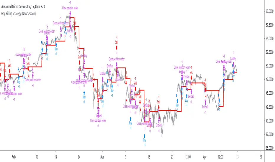
Strategy Builder Pro [ChartPrime]ChartPrime Strategy Creator Overview
The ChartPrime Strategy Builder offers traders an innovative, structured approach to building and testing strategies. The Strategy Creator allows users to combine, test, and automate complex strategies with many parameters.
Key Features of the ChartPrime Strategy Builder
1. Customizable Buy and Sell Conditions
The Strategy Creator provides flexibility in establishing entry and exit rules, with separate sections for long and short strategies. Traders can combine multiple conditions in each section to fine-tune when positions are opened or closed. For instance, they might choose to only buy when the indicator signals a buy and the Dynamic Reactor (a low lag filter) indicator shows a bullish trend. Users are able to pick, mix and match the following list of features:
Signal Mode: Select the type of assistive signals you are requiring. Provided are both trend following signals with self optimization using backtest results as well as reversal signals, aiming to provide real time tops and bottoms in markets. Both these signal modes can be fine tuned using the tuning input to refine signals to a trader's liking. ChartPrime Trend Signals leverage audio engineering inspired techniques and low-pass filters in order to achieve and attempt to produce lower lag response times and therefore are designed to have a uniqueness when compared to more classical trend following approaches.
The Dynamic Reactor: provides a simple band passing through the chart. This can provide assistance in support and resistance locations as well as identifying the trend direction expressed via green and red colors. Taking a moving average and applying unique adaptivity calculations gives this plot a unique and fast behavior.
Candlestick structures: analyze candlestick formation putting a spin on classical candlestick patterns and provide the most relevant formations on the chart. These are not classical and are filtered by further analyzing market activity. A trader's classic with a spin.
The Prime Trend Assistant: provides a trend following dynamic support and resistance level. This makes it perfect to use in confluence or as a filter for other supporting indicators. This is an adaptive trend following system designed to handle volatility leveraging filter kernels as opposed to low pass filters.
Money Flow: with further filters applied for early response to money flow changes in the market. This can be a great filter in trends.
Oscillator reversals: are built in leveraging an oscillator focusing on market momentum allowing users to enter based on market shifts and trends along with reversals.
Volume-Inspired Signals: determine overbought and oversold conditions, adding another layer of analysis to the oscillator. These appear as orange labels, providing a simple reading into a possible reversal.
The Volume Matrix: is a volume oscillator that shows whether money is flowing into or out of the market. Green suggests an uptrend with buyers in control, while red indicates a majority of sellers. By incorporating smoothed volume analysis, it distinguishes between bullish and bearish volumes, offering an early indication of potential trend reversals.
The True 7: is a middle-ranking system that evaluates the strength of a move and the overall trend, offering a numeric or visual representation of trend strength. It can also indicate when a trend is starting to reverse, providing leading signals for potential market shifts. Rather than using an oscillator, this offers the unique edge of falling into set categories, making understanding it simple. This can be a great confluence point when designing a strategy.
Take profits: These offer real-time suggestions from our algorithm on when it might be a good time to take profit. Using these as part of a strategy allows for great entries at bottoms and tops of trends.
Using features such as the Dynamic reactor have dual purposes. Traders can use this as both a filter and an entry condition. This allows for true interoperability when using the Strategy Builder. The above conditions are duplicated for short entries too allowing for symmetrical trading systems. By disabling all of the entry conditions on either long or short areas of the settings will create a strategy that only takes a single type of position. For example; a trader that just wants to take longs can disable all short options.
2. Layered Entries
Layered entries, a feature to enhance the uniqueness in the tool. It allows traders to average into positions as the market moves, rather than committing all capital at once. This feature is particularly useful for volatile markets where prices may fluctuate substantially. The Strategy Builder lets users adjust the number of layered entries, which can help in managing risk and optimizing entry points as well as the aggressiveness of the safety orders. With each safety order placed the system will automatically and dynamically scale into positions reducing the average entry price and hence dynamically adjust the potential take profits. Due to the potential complexities of exiting during multiple orders, a smart system is employed to automatically take profits on the layered system aiming to take profits at peaks of trends.
Users are able to override this smart TP system at the bottom of the settings instead targeting percentage profits for both short and long positions.
Entries lowering average buy price
The ability to adjust how quickly the system layers into positions can also be adjusted via the layered entries drop down between fast and slow mode where the slow mode will be more cautious when producing new orders.
3. Flexible Take Profit (TP) and Stop Loss (SL) Options
Traders can set their TP and SL levels according to various parameters, including ATR (Average True Range), risk-reward ratio, trailing stops, or specific price changes. If layered entries are active, an automatic TP method is applied by default, though traders can manually specify TP values if they prefer. This setup allows for precise control over trade exits, tailored to the strategy’s risk profile.
Provided options
The ability to use external take profits and stop losses is also provided. By loading an indicator of your choice the plots will be added to the chart. By navigating to the external sources area of the settings, users can select this plot and use it as part of a wider trading system.
Example: Let’s say a user has entries based on the inbuilt trend signals and wishes to exit whenever the RSI crosses above 70, they can add RSI to the chart, select crossing up and enter the value of 70.
4. Integrated Reinvestment for Compounding Gains
The reinvestment option allows traders to reinvest a portion of their gains into future trades, increasing trade size over time and benefiting from compounding. For example, a user might set 30% of each trade's profit to reinvest, with the remaining 70% allocated for risk management or additional safety orders. This approach can enhance long-term growth while balancing risk.
Generally in trading it can be a good approach to take profits so we suggest a healthy balance. This setting is generally best used for slow steady strategies with the long term aim of accumulating as much of the asset as possible.
5. Leverage and Position Sizing
Users can configure leverage and position sizing to simulate varying risk levels and capital allocations. A dashboard on the interface displays margin requirements based on the selected leverage, allowing traders to estimate trade sizes relative to their available capital. Whenever using leverage especially with layered entries it’s important to keep a close eye on the position sizes to avoid potential liquidations.
6. Pre-Configured Strategies for Immediate Testing
For users seeking a starting point, ChartPrime includes a range of preset strategies. These were developed and backtested by ChartPrime’s team. This allows traders to start with a stable base and adapt it to their own preferences. It is vital to understand that historical performance doesn't guarantee future success, and traders should be mindful of overfitting. These pre-built configurations offer a structured way and base to design strategies off of. These are also subject to changing results as new price action arrives and they become outdated. They serve the purpose of simply being example use cases.
7. In-Depth Specific Backtesting Ranges
The Strategy Builder includes backtesting capabilities, providing a clear view of how different setups would have performed over specified time periods. Traders can select date ranges to target specific market conditions, then review results on TradingView to see how their strategies perform across different market trends.
Example Use Case: Developing a Strategy
Consider a trader who is focused on long positions only and prefers a lower-risk strategy (note these tools can be used for all assets; we are using an undisclosed asset as an example). Using the Strategy Builder, they could:
- Disable short conditions.
- Set long entry rules to trigger when both the ChartPrime oscillator and Quantum Reactor indicators show bullish signals.
- Enable layered entries to improve average entry prices by adding to positions during market dips.
- Run a backtest over a two-year period to see historical performance trends, making adjustments as needed.
The backtest will show where entries and exits would have occurred and how layered entries may have impacted profitability.
8. Iterative design
Strategy builders and creating a strategy is often an iterative process. By experimenting and using logic; a trader can arrive at a more sustainable system. Analyzing the shortcomings of your strategy and iteratively designing and filtering them out is the goal. For example; let’s say a strategy has high drawdown, a user would want to tighten stop losses for example to reduce this and find a balance point between optimizing winning trades and reducing the drawdown. When designing a strategy there are generally tradeoffs and optimizing taking into consideration a wide range of factors is key. This also applies to filtering techniques, entries and exits and every variable in the strategy.
Let’s say a strategy was taking too many long positions in a downtrend and after you’ve analyzed the data, you come to the conclusion this needs to be solved. Filtering these using built in trend following tools can be a great approach and refining with logic is a great approach.
The Strategy Builder also takes into consideration those who seek to automate especially via reinvesting and leverage features.
Considerations
The ChartPrime Strategy Builder aims to help traders build clear, rule-based strategies without excessive complexity. As with all backtesting tools, it's crucial to understand that historical performance doesn't guarantee future success, and traders should be mindful of overfitting. This tool offers a structured way to test strategies against various market conditions, helping traders refine their approaches with data-driven insights. Traders should also ensure they enter the correct fees when designing strategies and ensure usage on standard candle types.

Quantify [Entry Model] | FractalystWhat’s the indicator’s purpose and functionality?
Quantify is a machine learning entry model designed to help traders identify high-probability setups to refine their strategies.
➙ Simply pick your bias, select your entry timeframes, and let Quantify handle the rest for you.
Can the indicator be applied to any market approach/trading strategy?
Absolutely, all trading strategies share one fundamental element: Directional Bias
Once you’ve determined the market bias using your own personal approach, whether it’s through technical analysis or fundamental analysis, select the trend direction in the Quantify user inputs.
The algorithm will then adjust its calculations to provide optimal entry levels aligned with your chosen bias. This involves analyzing historical patterns to identify setups with the highest potential expected values, ensuring your setups are aligned with the selected direction.
Can the indicator be used for different timeframes or trading styles?
Yes, regardless of the timeframe you’d like to take your entries, the indicator adapts to your trading style.
Whether you’re a swing trader, scalper, or even a position trader, the algorithm dynamically evaluates market conditions across your chosen timeframe.
How can this indicator help me to refine my trading strategy?
1. Focus on Positive Expected Value
• The indicator evaluates every setup to ensure it has a positive expected value, helping you focus only on trades that statistically favor long-term profitability.
2. Adapt to Market Conditions
• By analyzing real-time market behavior and historical patterns, the algorithm adjusts its calculations to match current conditions, keeping your strategy relevant and adaptable.
3. Eliminate Emotional Bias
• With clear probabilities, expected values, and data-driven insights, the indicator removes guesswork and helps you avoid emotional decisions that can damage your edge.
4. Optimize Entry Levels
• The indicator identifies optimal entry levels based on your selected bias and timeframes, improving robustness in your trades.
5. Enhance Risk Management
• Using tools like the Kelly Criterion, the indicator suggests optimal position sizes and risk levels, ensuring that your strategy maintains consistency and discipline.
6. Avoid Overtrading
• By highlighting only high-potential setups, the indicator keeps you focused on quality over quantity, helping you refine your strategy and avoid unnecessary losses.
How can I get started to use the indicator for my entries?
1. Set Your Market Bias
• Determine whether the market trend is Bullish or Bearish using your own approach.
• Select the corresponding bias in the indicator’s user inputs to align it with your analysis.
2. Choose Your Entry Timeframes
• Specify the timeframes you want to focus on for trade entries.
• The indicator will dynamically analyze these timeframes to provide optimal setups.
3. Let the Algorithm Analyze
• Quantify evaluates historical data and real-time price action to calculate probabilities and expected values.
• It highlights setups with the highest potential based on your selected bias and timeframes.
4. Refine Your Entries
• Use the insights provided—entry levels, probabilities, and risk calculations—to align your trades with a math-driven edge.
• Avoid overtrading by focusing only on setups with positive expected value.
5. Adapt to Market Conditions
• The indicator continuously adapts to real-time market behavior, ensuring its recommendations stay relevant and precise as conditions change.
How does the indicator calculate the current range?
The indicator calculates the current range by analyzing swing points from the very first bar on your charts to the latest available bar it identifies external liquidity levels, also known as BSLQ (buy-side liquidity levels) and SSLQ (sell-side liquidity levels).
What's the purpose of these levels? What are the underlying calculations?
1. Understanding Swing highs and Swing Lows
Swing High: A Swing High is formed when there is a high with 2 lower highs to the left and right.
Swing Low: A Swing Low is formed when there is a low with 2 higher lows to the left and right.
2. Understanding the purpose and the underlying calculations behind Buyside, Sellside and Pivot levels.
3. Identifying Discount and Premium Zones.
4. Importance of Risk-Reward in Premium and Discount Ranges
How does the script calculate probabilities?
The script calculates the probability of each liquidity level individually. Here's the breakdown:
1. Upon the formation of a new range, the script waits for the price to reach and tap into pivot level level. Status: "■" - Inactive
2. Once pivot level is tapped into, the pivot status becomes activated and it waits for either liquidity side to be hit. Status: "▶" - Active
3. If the buyside liquidity is hit, the script adds to the count of successful buyside liquidity occurrences. Similarly, if the sellside is tapped, it records successful sellside liquidity occurrences.
4. Finally, the number of successful occurrences for each side is divided by the overall count individually to calculate the range probabilities.
Note: The calculations are performed independently for each directional range. A range is considered bearish if the previous breakout was through a sellside liquidity. Conversely, a range is considered bullish if the most recent breakout was through a buyside liquidity.
What does the multi-timeframe functionality offer?
You can incorporate up to 4 higher timeframe probabilities directly into the table.
This feature allows you to analyze the probabilities of buyside and sellside liquidity across multiple timeframes, without the need to manually switch between them.
By viewing these higher timeframe probabilities in one place, traders can spot larger market trends and refine their entries and exits with a better understanding of the overall market context.
What are the multi-timeframe underlying calculations?
The script uses the same calculations (mentioned above) and uses security function to request the data such as price levels, bar time, probabilities and booleans from the user-input timeframe.
How does the Indicator Identifies Positive Expected Values?
Quantify instantly calculates whether a trade setup has the potential to generate positive expected value (EV).
To determine a positive EV setup, the indicator uses the formula:
EV = ( P(Win) × R(Win) ) − ( P(Loss) × R(Loss))
where:
- P(Win) is the probability of a winning trade.
- R(Win) is the reward or return for a winning trade, determined by the current risk-to-reward ratio (RR).
- P(Loss) is the probability of a losing trade.
- R(Loss) is the loss incurred per losing trade, typically assumed to be -1.
By calculating these values based on historical data and the current trading setup, the indicator helps you understand whether your trade has a positive expected value.
How can I know that the setup I'm going to trade with has a positive EV?
If the indicator detects that the adjusted pivot and buy/sell side probabilities have generated positive expected value (EV) in historical data, the risk-to-reward (RR) label within the range box will be colored blue and red .
If the setup does not produce positive EV, the RR label will appear gray.
This indicates that even the risk-to-reward ratio is greater than 1:1, the setup is not likely to yield a positive EV because, according to historical data, the number of losses outweighs the number of wins relative to the RR gain per winning trade.
What is the confidence level in the indicator, and how is it determined?
The confidence level in the indicator reflects the reliability of the probabilities calculated based on historical data. It is determined by the sample size of the probabilities used in the calculations. A larger sample size generally increases the confidence level, indicating that the probabilities are more reliable and consistent with past performance.
How does the confidence level affect the risk-to-reward (RR) label?
The confidence level (★) is visually represented alongside the probability label. A higher confidence level indicates that the probabilities used to determine the RR label are based on a larger and more reliable sample size.
How can traders use the confidence level to make better trading decisions?
Traders can use the confidence level to gauge the reliability of the probabilities and expected value (EV) calculations provided by the indicator. A confidence level above 95% is considered statistically significant and indicates that the historical data supporting the probabilities is robust. This high confidence level suggests that the probabilities are reliable and that the indicator’s recommendations are more likely to be accurate.
In data science and statistics, a confidence level above 95% generally means that there is less than a 5% chance that the observed results are due to random variation. This threshold is widely accepted in research and industry as a marker of statistical significance. Studies such as those published in the Journal of Statistical Software and the American Statistical Association support this threshold, emphasizing that a confidence level above 95% provides a strong assurance of data reliability and validity.
Conversely, a confidence level below 95% indicates that the sample size may be insufficient and that the data might be less reliable. In such cases, traders should approach the indicator’s recommendations with caution and consider additional factors or further analysis before making trading decisions.
How does the sample size affect the confidence level, and how does it relate to my TradingView plan?
The sample size for calculating the confidence level is directly influenced by the amount of historical data available on your charts. A larger sample size typically leads to more reliable probabilities and higher confidence levels.
Here’s how the TradingView plans affect your data access:
Essential Plan
The Essential Plan provides basic data access with a limited amount of historical data. This can lead to smaller sample sizes and lower confidence levels, which may weaken the robustness of your probability calculations. Suitable for casual traders who do not require extensive historical analysis.
Plus Plan
The Plus Plan offers more historical data than the Essential Plan, allowing for larger sample sizes and more accurate confidence levels. This enhancement improves the reliability of indicator calculations. This plan is ideal for more active traders looking to refine their strategies with better data.
Premium Plan
The Premium Plan grants access to extensive historical data, enabling the largest sample sizes and the highest confidence levels. This plan provides the most reliable data for accurate calculations, with up to 20,000 historical bars available for analysis. It is designed for serious traders who need comprehensive data for in-depth market analysis.
PRO+ Plans
The PRO+ Plans offer the most extensive historical data, allowing for the largest sample sizes and the highest confidence levels. These plans are tailored for professional traders who require advanced features and significant historical data to support their trading strategies effectively.
For many traders, the Premium Plan offers a good balance of affordability and sufficient sample size for accurate confidence levels.
What is the HTF probability table and how does it work?
The HTF (Higher Time Frame) probability table is a feature that allows you to view buy and sellside probabilities and their status from timeframes higher than your current chart timeframe.
Here’s how it works:
Data Request: The table requests and retrieves data from user-defined higher timeframes (HTFs) that you select.
Probability Display: It displays the buy and sellside probabilities for each of these HTFs, providing insights into the likelihood of price movements based on higher timeframe data.
Detailed Tooltips: The table includes detailed tooltips for each timeframe, offering additional context and explanations to help you understand the data better.
What do the different colors in the HTF probability table indicate?
The colors in the HTF probability table provide visual cues about the expected value (EV) of trading setups based on higher timeframe probabilities:
Blue: Suggests that entering a long position from the HTF user-defined pivot point, targeting buyside liquidity, is likely to result in a positive expected value (EV) based on historical data and sample size.
Red: Indicates that entering a short position from the HTF user-defined pivot point, targeting sellside liquidity, is likely to result in a positive expected value (EV) based on historical data and sample size.
Gray: Shows that neither long nor short trades from the HTF user-defined pivot point are expected to generate positive EV, suggesting that trading these setups may not be favorable.
What machine learning techniques are used in Quantify?
Quantify offers two main machine learning approaches:
1. Adaptive Learning (Fixed Sample Size): The algorithm learns from the entire dataset without resampling, maintaining a stable model that adapts to the latest market conditions.
2. Bootstrap Resampling: This method creates multiple subsets of the historical data, allowing the model to train on varying sample sizes. This technique enhances the robustness of predictions by ensuring that the model is not overfitting to a single dataset.
How does machine learning affect the expected value calculations in Quantify?
Machine learning plays a key role in improving the accuracy of expected value (EV) calculations. By analyzing historical price action, liquidity hits, and market bias patterns, the model continuously adjusts its understanding of risk and reward, allowing the expected value to reflect the most likely market movements. This results in more precise EV predictions, helping traders focus on setups that maximize profitability.
What is the Kelly Criterion, and how does it work in Quantify?
The Kelly Criterion is a mathematical formula used to determine the optimal position size for each trade, maximizing long-term growth while minimizing the risk of large drawdowns. It calculates the percentage of your portfolio to risk on a trade based on the probability of winning and the expected payoff.
Quantify integrates this with user-defined inputs to dynamically calculate the most effective position size in percentage, aligning with the trader’s risk tolerance and desired exposure.
How does Quantify use the Kelly Criterion in practice?
Quantify uses the Kelly Criterion to optimize position sizing based on the following factors:
1. Confidence Level: The model assesses the confidence level in the trade setup based on historical data and sample size. A higher confidence level increases the suggested position size because the trade has a higher probability of success.
2. Max Allowed Drawdown (User-Defined): Traders can set their preferred maximum allowed drawdown, which dictates how much loss is acceptable before reducing position size or stopping trading. Quantify uses this input to ensure that risk exposure aligns with the trader’s risk tolerance.
3. Probabilities: Quantify calculates the probabilities of success for each trade setup. The higher the probability of a successful trade (based on historical price action and liquidity levels), the larger the position size suggested by the Kelly Criterion.
What is a trailing stoploss, and how does it work in Quantify?
A trailing stoploss is a dynamic risk management tool that moves with the price as the market trend continues in the trader’s favor. Unlike a fixed take profit, which stays at a set level, the trailing stoploss automatically adjusts itself as the market moves, locking in profits as the price advances.
In Quantify, the trailing stoploss is enhanced by incorporating market structure liquidity levels (explain above). This ensures that the stoploss adjusts intelligently based on key price levels, allowing the trader to stay in the trade as long as the trend remains intact, while also protecting profits if the market reverses.
Why would a trader prefer a trailing stoploss based on liquidity levels instead of a fixed take-profit level?
Traders who use trailing stoplosses based on liquidity levels prefer this method because:
1. Market-Driven Flexibility: The stoploss follows the market structure rather than being static at a pre-defined level. This means the stoploss is less likely to be hit by small market fluctuations or false reversals. The stoploss remains adaptive, moving as the market moves.
2. Riding the Trend: Traders can capture more profit during a sustained trend because the trailing stop will adjust only when the trend starts to reverse significantly, based on key liquidity levels. This allows them to hold positions longer without prematurely locking in profits.
3. Avoiding Premature Exits: Fixed stoploss levels may exit a trade too early in volatile markets, while liquidity-based trailing stoploss levels respect the natural flow of price action, preventing the trader from exiting too soon during pullbacks or minor retracements.
🎲 Becoming the House: Gaining an Edge Over the Market
In American roulette, the casino has a 5.26% edge due to the presence of the 0 and 00 pockets. On even-money bets, players face a 47.37% chance of winning, while true 50/50 odds would require a 50% chance. This edge—the gap between the payout odds and the true probabilities—ensures that, statistically, the casino will always win over time, even if individual players win occasionally.
From a Trader’s Perspective
In trading, your edge comes from identifying and executing setups with a positive expected value (EV). For example:
• If you identify a setup with a 55.48% chance of winning and a 1:1 risk-to-reward (RR) ratio, your trade has a statistical advantage over a neutral (50/50) probability.
This edge works in your favor when applied consistently across a series of trades, just as the casino’s edge ensures profitability across thousands of spins.
🎰 Applying the Concept to Trading
Like casinos leverage their mathematical edge in games of chance, you can achieve long-term success in trading by focusing on setups with positive EV and managing your trades systematically. Here’s how:
1. Probability Advantage: Prioritize trades where the probability of success (win rate) exceeds the breakeven rate for your chosen risk-to-reward ratio.
• Example: With a 1:1 RR, you need a win rate above 50% to achieve positive EV.
2. Risk-to-Reward Ratio (RR): Even with a win rate below 50%, you can gain an edge by increasing your RR (e.g., a 40% win rate with a 2:1 RR still has positive EV).
3. Consistency and Discipline: Just as casinos profit by sticking to their mathematical advantage over thousands of spins, traders must rely on their edge across many trades, avoiding emotional decisions or overleveraging.
By targeting favorable probabilities and managing trades effectively, you “become the house” in your trading. This approach allows you to leverage statistical advantages to enhance your overall performance and achieve sustainable profitability.
What Makes the Quantify Indicator Original?
1. Data-Driven Edge
Unlike traditional indicators that rely on static formulas, Quantify leverages probability-based analysis and machine learning. It calculates expected value (EV) and confidence levels to help traders identify setups with a true statistical edge.
2. Integration of Market Structure
Quantify uses market structure liquidity levels to dynamically adapt. It identifies key zones like swing highs/lows and liquidity traps, enabling users to align entries and exits with where the market is most likely to react. This bridges the gap between price action analysis and quantitative trading.
3. Sophisticated Risk Management
The Kelly Criterion implementation is unique. Quantify allows traders to input their maximum allowed drawdown, dynamically adjusting risk exposure to maintain optimal position sizing. This ensures risk is scientifically controlled while maximizing potential growth.
4. Multi-Timeframe and Liquidity-Based Trailing Stops
The indicator doesn’t just suggest fixed profit-taking levels. It offers market structure-based trailing stop-loss functionality, letting traders ride trends as long as liquidity and probabilities favor the position, which is rare in most tools.
5. Customizable Bias and Adaptive Learning
• Directional Bias: Traders can set a bullish or bearish bias, and the indicator recalculates probabilities to align with the trader’s market outlook.
• Adaptive Learning: The machine learning model adapts to changes in data (via resampling or bootstrap methods), ensuring that predictions stay relevant in evolving markets.
6. Positive EV Focus
The focus on positive EV setups differentiates it from reactive indicators. It shifts trading from chasing signals to acting on setups that statistically favor profitability, akin to how professional quant funds operate.
7. User Empowerment
Through features like customizable timeframes, real-time probability updates, and visualization tools, Quantify empowers users to make data-informed decisions.
Terms and Conditions | Disclaimer
Our charting tools are provided for informational and educational purposes only and should not be construed as financial, investment, or trading advice. They are not intended to forecast market movements or offer specific recommendations. Users should understand that past performance does not guarantee future results and should not base financial decisions solely on historical data.
Built-in components, features, and functionalities of our charting tools are the intellectual property of @Fractalyst use, reproduction, or distribution of these proprietary elements is prohibited.
By continuing to use our charting tools, the user acknowledges and accepts the Terms and Conditions outlined in this legal disclaimer and agrees to respect our intellectual property rights and comply with all applicable laws and regulations.

GKD-BT Multi-Ticker Baseline Backtest [Loxx]The Giga Kaleidoscope GKD-BT Multi-Ticker Baseline Backtest is a backtesting module included in Loxx's "Giga Kaleidoscope Modularized Trading System."
█ Giga Kaleidoscope GKD-BT Multi-Ticker Baseline Backtest
The Multi-Ticker SCSC Backtest is a Solo Confirmation Super Complex backtest that allows traders to test GKD-B Multi-Ticker Baseline series baselines indicators filtered. The purpose of this backtest is to enable traders to quickly evaluate the viability of a Baseline across hundreds of tickers within 30-60 minutes.
The backtest module supports testing with 1 take profit and 1 stop loss. It also offers the option to limit testing to a specific date range, allowing simulated forward testing using historical data. This backtest module only includes standard long and short signals. Additionally, users can choose to display or hide a trading panel that provides relevant information about the backtest, statistics, and the current trade. Traders can also select a highlighting threshold for Total Percent Wins and Percent Profitable, and Profit Factor.
To use this indicator:
1. Import 1-10 tickers into the GKD-B Multi-Ticker Baseline indicator
2. Import the value "Input into NEW GKD-BT Multi-ticker Backtest" from the GKD-B Multi-Ticker Baseline indicator (Volatility-Adaptive, Stepped, etc.) into the GKD-BT Multi-Ticker Baseline Backtest.
3. Import the same 1-10 tickers from number step 1 above into the GKD-BT Multi-Ticker Baseline Backtest indicator into the text area field "Input Tickers separated by commas".
3. When importing tickers, ensure that you import the same type of tickers for all 1-10 tickers. For example, test only FX or Cryptocurrency or Stocks. Do not combine different tradable asset types.
4. Make sure that your chart is set to a ticker that corresponds to the tradable asset type. For cryptocurrency testing, set the chart to BTCUSDT. For Forex testing, set the chart to EURUSD.
This backtest includes the following metrics:
1. Net profit: Overall profit or loss achieved.
2. Total Closed Trades: Total number of closed trades, both winning and losing.
3. Total Percent Wins: Total wins, whether long or short, for the selected time interval regardless of commissions and other profit-modifying add-ons.
4. Percent Profitable: Total wins, whether long or short, that are also profitable, taking commissions into account.
5. Profit Factor: The ratio of gross profits to gross losses, indicating how much money the strategy made for every unit of money it lost.
6. Average Profit per Trade: The average gain or loss per trade, calculated by dividing the net profit by the total number of closed trades.
7. Average Number of Bars in Trade: The average number of bars that elapsed during trades for all closed trades.
Summary of notable settings:
Input Tickers separated by commas: Allows the user to input tickers separated by commas, specifying the symbols or tickers of financial instruments used in the backtest. The tickers should follow the format "EXCHANGE:TICKER" (e.g., "NASDAQ:AAPL, NYSE:MSFT").
Import GKD-B Baseline: Imports the "GKD-B Multi-Ticker Baseline" indicator.
Initial Capital: Represents the starting account balance for the backtest, denominated in the base currency of the trading account.
Order Size: Determines the quantity of contracts traded in each trade.
Order Type: Specifies the type of order used in the backtest, either "Contracts" or "% Equity."
Commission: Represents the commission per order or transaction cost incurred in each trade.
**the backtest data rendered to the chart above uses $5 commission per trade and 10% equity per trade with $1 million initial capital. Each backtest result for each ticker assumes these same inputs. The results are NOT cumulative, they are separate and isolated per ticker and trading side, long or short**
█ Volatility Types included
The GKD system utilizes volatility-based take profits and stop losses. Each take profit and stop loss is calculated as a multiple of volatility. You can change the values of the multipliers in the settings as well.
This module includes 17 types of volatility:
Close-to-Close
Parkinson
Garman-Klass
Rogers-Satchell
Yang-Zhang
Garman-Klass-Yang-Zhang
Exponential Weighted Moving Average
Standard Deviation of Log Returns
Pseudo GARCH(2,2)
Average True Range
True Range Double
Standard Deviation
Adaptive Deviation
Median Absolute Deviation
Efficiency-Ratio Adaptive ATR
Mean Absolute Deviation
Static Percent
Various volatility estimators and indicators that investors and traders can use to measure the dispersion or volatility of a financial instrument's price. Each estimator has its strengths and weaknesses, and the choice of estimator should depend on the specific needs and circumstances of the user.
Close-to-Close
Close-to-Close volatility is a classic and widely used volatility measure, sometimes referred to as historical volatility.
Volatility is an indicator of the speed of a stock price change. A stock with high volatility is one where the price changes rapidly and with a larger amplitude. The more volatile a stock is, the riskier it is.
Close-to-close historical volatility is calculated using only a stock's closing prices. It is the simplest volatility estimator. However, in many cases, it is not precise enough. Stock prices could jump significantly during a trading session and return to the opening value at the end. That means that a considerable amount of price information is not taken into account by close-to-close volatility.
Despite its drawbacks, Close-to-Close volatility is still useful in cases where the instrument doesn't have intraday prices. For example, mutual funds calculate their net asset values daily or weekly, and thus their prices are not suitable for more sophisticated volatility estimators.
Parkinson
Parkinson volatility is a volatility measure that uses the stock’s high and low price of the day.
The main difference between regular volatility and Parkinson volatility is that the latter uses high and low prices for a day, rather than only the closing price. This is useful as close-to-close prices could show little difference while large price movements could have occurred during the day. Thus, Parkinson's volatility is considered more precise and requires less data for calculation than close-to-close volatility.
One drawback of this estimator is that it doesn't take into account price movements after the market closes. Hence, it systematically undervalues volatility. This drawback is addressed in the Garman-Klass volatility estimator.
Garman-Klass
Garman-Klass is a volatility estimator that incorporates open, low, high, and close prices of a security.
Garman-Klass volatility extends Parkinson's volatility by taking into account the opening and closing prices. As markets are most active during the opening and closing of a trading session, it makes volatility estimation more accurate.
Garman and Klass also assumed that the process of price change follows a continuous diffusion process (Geometric Brownian motion). However, this assumption has several drawbacks. The method is not robust for opening jumps in price and trend movements.
Despite its drawbacks, the Garman-Klass estimator is still more effective than the basic formula since it takes into account not only the price at the beginning and end of the time interval but also intraday price extremes.
Researchers Rogers and Satchell have proposed a more efficient method for assessing historical volatility that takes into account price trends. See Rogers-Satchell Volatility for more detail.
Rogers-Satchell
Rogers-Satchell is an estimator for measuring the volatility of securities with an average return not equal to zero.
Unlike Parkinson and Garman-Klass estimators, Rogers-Satchell incorporates a drift term (mean return not equal to zero). As a result, it provides better volatility estimation when the underlying is trending.
The main disadvantage of this method is that it does not take into account price movements between trading sessions. This leads to an underestimation of volatility since price jumps periodically occur in the market precisely at the moments between sessions.
A more comprehensive estimator that also considers the gaps between sessions was developed based on the Rogers-Satchel formula in the 2000s by Yang-Zhang. See Yang Zhang Volatility for more detail.
Yang-Zhang
Yang Zhang is a historical volatility estimator that handles both opening jumps and the drift and has a minimum estimation error.
Yang-Zhang volatility can be thought of as a combination of the overnight (close-to-open volatility) and a weighted average of the Rogers-Satchell volatility and the day’s open-to-close volatility. It is considered to be 14 times more efficient than the close-to-close estimator.
Garman-Klass-Yang-Zhang
Garman-Klass-Yang-Zhang (GKYZ) volatility estimator incorporates the returns of open, high, low, and closing prices in its calculation.
GKYZ volatility estimator takes into account overnight jumps but not the trend, i.e., it assumes that the underlying asset follows a Geometric Brownian Motion (GBM) process with zero drift. Therefore, the GKYZ volatility estimator tends to overestimate the volatility when the drift is different from zero. However, for a GBM process, this estimator is eight times more efficient than the close-to-close volatility estimator.
Exponential Weighted Moving Average
The Exponentially Weighted Moving Average (EWMA) is a quantitative or statistical measure used to model or describe a time series. The EWMA is widely used in finance, with the main applications being technical analysis and volatility modeling.
The moving average is designed such that older observations are given lower weights. The weights decrease exponentially as the data point gets older – hence the name exponentially weighted.
The only decision a user of the EWMA must make is the parameter lambda. The parameter decides how important the current observation is in the calculation of the EWMA. The higher the value of lambda, the more closely the EWMA tracks the original time series.
Standard Deviation of Log Returns
This is the simplest calculation of volatility. It's the standard deviation of ln(close/close(1)).
Pseudo GARCH(2,2)
This is calculated using a short- and long-run mean of variance multiplied by ?.
avg(var;M) + (1 ? ?) avg(var;N) = 2?var/(M+1-(M-1)L) + 2(1-?)var/(M+1-(M-1)L)
Solving for ? can be done by minimizing the mean squared error of estimation; that is, regressing L^-1var - avg(var; N) against avg(var; M) - avg(var; N) and using the resulting beta estimate as ?.
Average True Range
The average true range (ATR) is a technical analysis indicator, introduced by market technician J. Welles Wilder Jr. in his book New Concepts in Technical Trading Systems, that measures market volatility by decomposing the entire range of an asset price for that period.
The true range indicator is taken as the greatest of the following: current high less the current low; the absolute value of the current high less the previous close; and the absolute value of the current low less the previous close. The ATR is then a moving average, generally using 14 days, of the true ranges.
True Range Double
A special case of ATR that attempts to correct for volatility skew.
Standard Deviation
Standard deviation is a statistic that measures the dispersion of a dataset relative to its mean and is calculated as the square root of the variance. The standard deviation is calculated as the square root of variance by determining each data point's deviation relative to the mean. If the data points are further from the mean, there is a higher deviation within the data set; thus, the more spread out the data, the higher the standard deviation.
Adaptive Deviation
By definition, the Standard Deviation (STD, also represented by the Greek letter sigma ? or the Latin letter s) is a measure that is used to quantify the amount of variation or dispersion of a set of data values. In technical analysis, we usually use it to measure the level of current volatility.
Standard Deviation is based on Simple Moving Average calculation for mean value. This version of standard deviation uses the properties of EMA to calculate what can be called a new type of deviation, and since it is based on EMA, we can call it EMA deviation. Additionally, Perry Kaufman's efficiency ratio is used to make it adaptive (since all EMA type calculations are nearly perfect for adapting).
The difference when compared to the standard is significant--not just because of EMA usage, but the efficiency ratio makes it a "bit more logical" in very volatile market conditions.
Median Absolute Deviation
The median absolute deviation is a measure of statistical dispersion. Moreover, the MAD is a robust statistic, being more resilient to outliers in a data set than the standard deviation. In the standard deviation, the distances from the mean are squared, so large deviations are weighted more heavily, and thus outliers can heavily influence it. In the MAD, the deviations of a small number of outliers are irrelevant.
Because the MAD is a more robust estimator of scale than the sample variance or standard deviation, it works better with distributions without a mean or variance, such as the Cauchy distribution.
For this indicator, a manual recreation of the quantile function in Pine Script is used. This is so users have a full inside view into how this is calculated.
Efficiency-Ratio Adaptive ATR
Average True Range (ATR) is a widely used indicator for many occasions in technical analysis. It is calculated as the RMA of the true range. This version adds a "twist": it uses Perry Kaufman's Efficiency Ratio to calculate adaptive true range.
Mean Absolute Deviation
The mean absolute deviation (MAD) is a measure of variability that indicates the average distance between observations and their mean. MAD uses the original units of the data, which simplifies interpretation. Larger values signify that the data points spread out further from the average. Conversely, lower values correspond to data points bunching closer to it. The mean absolute deviation is also known as the mean deviation and average absolute deviation.
This definition of the mean absolute deviation sounds similar to the standard deviation (SD). While both measure variability, they have different calculations. In recent years, some proponents of MAD have suggested that it replace the SD as the primary measure because it is a simpler concept that better fits real life.
█ Giga Kaleidoscope Modularized Trading System
Core components of an NNFX algorithmic trading strategy
The NNFX algorithm is built on the principles of trend, momentum, and volatility. There are six core components in the NNFX trading algorithm:
1. Volatility - price volatility; e.g., Average True Range, True Range Double, Close-to-Close, etc.
2. Baseline - a moving average to identify price trend
3. Confirmation 1 - a technical indicator used to identify trends
4. Confirmation 2 - a technical indicator used to identify trends
5. Continuation - a technical indicator used to identify trends
6. Volatility/Volume - a technical indicator used to identify volatility/volume breakouts/breakdown
7. Exit - a technical indicator used to determine when a trend is exhausted
8. Metamorphosis - a technical indicator that produces a compound signal from the combination of other GKD indicators*
*(not part of the NNFX algorithm)
What is Volatility in the NNFX trading system?
In the NNFX (No Nonsense Forex) trading system, ATR (Average True Range) is typically used to measure the volatility of an asset. It is used as a part of the system to help determine the appropriate stop loss and take profit levels for a trade. ATR is calculated by taking the average of the true range values over a specified period.
True range is calculated as the maximum of the following values:
-Current high minus the current low
-Absolute value of the current high minus the previous close
-Absolute value of the current low minus the previous close
ATR is a dynamic indicator that changes with changes in volatility. As volatility increases, the value of ATR increases, and as volatility decreases, the value of ATR decreases. By using ATR in NNFX system, traders can adjust their stop loss and take profit levels according to the volatility of the asset being traded. This helps to ensure that the trade is given enough room to move, while also minimizing potential losses.
Other types of volatility include True Range Double (TRD), Close-to-Close, and Garman-Klass
What is a Baseline indicator?
The baseline is essentially a moving average, and is used to determine the overall direction of the market.
The baseline in the NNFX system is used to filter out trades that are not in line with the long-term trend of the market. The baseline is plotted on the chart along with other indicators, such as the Moving Average (MA), the Relative Strength Index (RSI), and the Average True Range (ATR).
Trades are only taken when the price is in the same direction as the baseline. For example, if the baseline is sloping upwards, only long trades are taken, and if the baseline is sloping downwards, only short trades are taken. This approach helps to ensure that trades are in line with the overall trend of the market, and reduces the risk of entering trades that are likely to fail.
By using a baseline in the NNFX system, traders can have a clear reference point for determining the overall trend of the market, and can make more informed trading decisions. The baseline helps to filter out noise and false signals, and ensures that trades are taken in the direction of the long-term trend.
What is a Confirmation indicator?
Confirmation indicators are technical indicators that are used to confirm the signals generated by primary indicators. Primary indicators are the core indicators used in the NNFX system, such as the Average True Range (ATR), the Moving Average (MA), and the Relative Strength Index (RSI).
The purpose of the confirmation indicators is to reduce false signals and improve the accuracy of the trading system. They are designed to confirm the signals generated by the primary indicators by providing additional information about the strength and direction of the trend.
Some examples of confirmation indicators that may be used in the NNFX system include the Bollinger Bands, the MACD (Moving Average Convergence Divergence), and the MACD Oscillator. These indicators can provide information about the volatility, momentum, and trend strength of the market, and can be used to confirm the signals generated by the primary indicators.
In the NNFX system, confirmation indicators are used in combination with primary indicators and other filters to create a trading system that is robust and reliable. By using multiple indicators to confirm trading signals, the system aims to reduce the risk of false signals and improve the overall profitability of the trades.
What is a Continuation indicator?
In the NNFX (No Nonsense Forex) trading system, a continuation indicator is a technical indicator that is used to confirm a current trend and predict that the trend is likely to continue in the same direction. A continuation indicator is typically used in conjunction with other indicators in the system, such as a baseline indicator, to provide a comprehensive trading strategy.
What is a Volatility/Volume indicator?
Volume indicators, such as the On Balance Volume (OBV), the Chaikin Money Flow (CMF), or the Volume Price Trend (VPT), are used to measure the amount of buying and selling activity in a market. They are based on the trading volume of the market, and can provide information about the strength of the trend. In the NNFX system, volume indicators are used to confirm trading signals generated by the Moving Average and the Relative Strength Index. Volatility indicators include Average Direction Index, Waddah Attar, and Volatility Ratio. In the NNFX trading system, volatility is a proxy for volume and vice versa.
By using volume indicators as confirmation tools, the NNFX trading system aims to reduce the risk of false signals and improve the overall profitability of trades. These indicators can provide additional information about the market that is not captured by the primary indicators, and can help traders to make more informed trading decisions. In addition, volume indicators can be used to identify potential changes in market trends and to confirm the strength of price movements.
What is an Exit indicator?
The exit indicator is used in conjunction with other indicators in the system, such as the Moving Average (MA), the Relative Strength Index (RSI), and the Average True Range (ATR), to provide a comprehensive trading strategy.
The exit indicator in the NNFX system can be any technical indicator that is deemed effective at identifying optimal exit points. Examples of exit indicators that are commonly used include the Parabolic SAR, and the Average Directional Index (ADX).
The purpose of the exit indicator is to identify when a trend is likely to reverse or when the market conditions have changed, signaling the need to exit a trade. By using an exit indicator, traders can manage their risk and prevent significant losses.
In the NNFX system, the exit indicator is used in conjunction with a stop loss and a take profit order to maximize profits and minimize losses. The stop loss order is used to limit the amount of loss that can be incurred if the trade goes against the trader, while the take profit order is used to lock in profits when the trade is moving in the trader's favor.
Overall, the use of an exit indicator in the NNFX trading system is an important component of a comprehensive trading strategy. It allows traders to manage their risk effectively and improve the profitability of their trades by exiting at the right time.
What is an Metamorphosis indicator?
The concept of a metamorphosis indicator involves the integration of two or more GKD indicators to generate a compound signal. This is achieved by evaluating the accuracy of each indicator and selecting the signal from the indicator with the highest accuracy. As an illustration, let's consider a scenario where we calculate the accuracy of 10 indicators and choose the signal from the indicator that demonstrates the highest accuracy.
The resulting output from the metamorphosis indicator can then be utilized in a GKD-BT backtest by occupying a slot that aligns with the purpose of the metamorphosis indicator. The slot can be a GKD-B, GKD-C, or GKD-E slot, depending on the specific requirements and objectives of the indicator. This allows for seamless integration and utilization of the compound signal within the GKD-BT framework.
How does Loxx's GKD (Giga Kaleidoscope Modularized Trading System) implement the NNFX algorithm outlined above?
Loxx's GKD v2.0 system has five types of modules (indicators/strategies). These modules are:
1. GKD-BT - Backtesting module (Volatility, Number 1 in the NNFX algorithm)
2. GKD-B - Baseline module (Baseline and Volatility/Volume, Numbers 1 and 2 in the NNFX algorithm)
3. GKD-C - Confirmation 1/2 and Continuation module (Confirmation 1/2 and Continuation, Numbers 3, 4, and 5 in the NNFX algorithm)
4. GKD-V - Volatility/Volume module (Confirmation 1/2, Number 6 in the NNFX algorithm)
5. GKD-E - Exit module (Exit, Number 7 in the NNFX algorithm)
6. GKD-M - Metamorphosis module (Metamorphosis, Number 8 in the NNFX algorithm, but not part of the NNFX algorithm)
(additional module types will added in future releases)
Each module interacts with every module by passing data to A backtest module wherein the various components of the GKD system are combined to create a trading signal.
That is, the Baseline indicator passes its data to Volatility/Volume. The Volatility/Volume indicator passes its values to the Confirmation 1 indicator. The Confirmation 1 indicator passes its values to the Confirmation 2 indicator. The Confirmation 2 indicator passes its values to the Continuation indicator. The Continuation indicator passes its values to the Exit indicator, and finally, the Exit indicator passes its values to the Backtest strategy.
This chaining of indicators requires that each module conform to Loxx's GKD protocol, therefore allowing for the testing of every possible combination of technical indicators that make up the six components of the NNFX algorithm.
What does the application of the GKD trading system look like?
Example trading system:
Backtest: Multi-Ticker CC Backtest
Baseline: Hull Moving Average
Volatility/Volume: Hurst Exponent
Confirmation 1: Advance Trend Pressure as shown on the chart above
Confirmation 2: uf2018
Continuation: Coppock Curve
Exit: Rex Oscillator
Metamorphosis: Baseline Optimizer
Each GKD indicator is denoted with a module identifier of either: GKD-BT, GKD-B, GKD-C, GKD-V, GKD-M, or GKD-E. This allows traders to understand to which module each indicator belongs and where each indicator fits into the GKD system.
█ Giga Kaleidoscope Modularized Trading System Signals
Standard Entry
1. GKD-C Confirmation gives signal
2. Baseline agrees
3. Price inside Goldie Locks Zone Minimum
4. Price inside Goldie Locks Zone Maximum
5. Confirmation 2 agrees
6. Volatility/Volume agrees
1-Candle Standard Entry
1a. GKD-C Confirmation gives signal
2a. Baseline agrees
3a. Price inside Goldie Locks Zone Minimum
4a. Price inside Goldie Locks Zone Maximum
Next Candle
1b. Price retraced
2b. Baseline agrees
3b. Confirmation 1 agrees
4b. Confirmation 2 agrees
5b. Volatility/Volume agrees
Baseline Entry
1. GKD-B Baseline gives signal
2. Confirmation 1 agrees
3. Price inside Goldie Locks Zone Minimum
4. Price inside Goldie Locks Zone Maximum
5. Confirmation 2 agrees
6. Volatility/Volume agrees
7. Confirmation 1 signal was less than 'Maximum Allowable PSBC Bars Back' prior
1-Candle Baseline Entry
1a. GKD-B Baseline gives signal
2a. Confirmation 1 agrees
3a. Price inside Goldie Locks Zone Minimum
4a. Price inside Goldie Locks Zone Maximum
5a. Confirmation 1 signal was less than 'Maximum Allowable PSBC Bars Back' prior
Next Candle
1b. Price retraced
2b. Baseline agrees
3b. Confirmation 1 agrees
4b. Confirmation 2 agrees
5b. Volatility/Volume agrees
Volatility/Volume Entry
1. GKD-V Volatility/Volume gives signal
2. Confirmation 1 agrees
3. Price inside Goldie Locks Zone Minimum
4. Price inside Goldie Locks Zone Maximum
5. Confirmation 2 agrees
6. Baseline agrees
7. Confirmation 1 signal was less than 7 candles prior
1-Candle Volatility/Volume Entry
1a. GKD-V Volatility/Volume gives signal
2a. Confirmation 1 agrees
3a. Price inside Goldie Locks Zone Minimum
4a. Price inside Goldie Locks Zone Maximum
5a. Confirmation 1 signal was less than 'Maximum Allowable PSVVC Bars Back' prior
Next Candle
1b. Price retraced
2b. Volatility/Volume agrees
3b. Confirmation 1 agrees
4b. Confirmation 2 agrees
5b. Baseline agrees
Confirmation 2 Entry
1. GKD-C Confirmation 2 gives signal
2. Confirmation 1 agrees
3. Price inside Goldie Locks Zone Minimum
4. Price inside Goldie Locks Zone Maximum
5. Volatility/Volume agrees
6. Baseline agrees
7. Confirmation 1 signal was less than 7 candles prior
1-Candle Confirmation 2 Entry
1a. GKD-C Confirmation 2 gives signal
2a. Confirmation 1 agrees
3a. Price inside Goldie Locks Zone Minimum
4a. Price inside Goldie Locks Zone Maximum
5a. Confirmation 1 signal was less than 'Maximum Allowable PSC2C Bars Back' prior
Next Candle
1b. Price retraced
2b. Confirmation 2 agrees
3b. Confirmation 1 agrees
4b. Volatility/Volume agrees
5b. Baseline agrees
PullBack Entry
1a. GKD-B Baseline gives signal
2a. Confirmation 1 agrees
3a. Price is beyond 1.0x Volatility of Baseline
Next Candle
1b. Price inside Goldie Locks Zone Minimum
2b. Price inside Goldie Locks Zone Maximum
3b. Confirmation 1 agrees
4b. Confirmation 2 agrees
5b. Volatility/Volume agrees
Continuation Entry
1. Standard Entry, 1-Candle Standard Entry, Baseline Entry, 1-Candle Baseline Entry, Volatility/Volume Entry, 1-Candle Volatility/Volume Entry, Confirmation 2 Entry, 1-Candle Confirmation 2 Entry, or Pullback entry triggered previously
2. Baseline hasn't crossed since entry signal trigger
4. Confirmation 1 agrees
5. Baseline agrees
6. Confirmation 2 agrees

GKD-BT Multi-Ticker CC Backtest [Loxx]The Giga Kaleidoscope GKD-BT Multi-Ticker CC Backtest is a backtest module included in Loxx's "Giga Kaleidoscope Modularized Trading System."
█ Giga Kaleidoscope GKD-BT Multi-Ticker CC Backtest
This backtest allows you to test GKD-C Confirmation 1 and GKD-C Confirmation 2 indicators together without the hassle of adding additional confluence indicators. The backtest includes 1 take profit and 1 SL and various types of volatility. The backtest results on the chart are using 10% equity of 1 million total equity and $5 commission per trade.
To use this indicator:
1. Import the value "Input into NEW GKD-BT Backtest" from the GKD-C Confirmation 1 indicator into the GKD-BT Multi-Ticker CC Backtest.
2. Import the value "Input into NEW GKD-BT Backtest" from the GKD-C Confirmation 2 indicator into the GKD-BT Multi-Ticker CC Backtest.
This backtest includes the following metrics:
1. Net profit: Overall profit or loss achieved.
2. Total Closed Trades: Total number of closed trades, both winning and losing.
3. Total Percent Wins: Total wins, whether long or short, for the selected time interval regardless of commissions and other profit-modifying addons.
4. Percent Profitable: Total wins, whether long or short, that are also profitable, taking commissions into account.
5. Profit Factor: The ratio of gross profits to gross losses, indicating how much money the strategy made for every unit of money it lost.
6. Average Profit per Trade: The average gain or loss per trade, calculated by dividing the net profit by the total number of closed trades.
7. Average Number of Bars in Trade: The average number of bars that elapsed during trades for all closed trades.
Summary of notable settings:
Input Tickers separated by commas: Allows the user to input tickers separated by commas, specifying the symbols or tickers of financial instruments used in the backtest. The tickers should follow the format "EXCHANGE:TICKER" (e.g., "NASDAQ:AAPL, NYSE:MSFT").
Import GKD-B Baseline: Imports the "GKD-B Baseline" indicator.
Import GKD-V Volatility/Volume: Imports the "GKD-V Volatility/Volume" indicator.
Import GKD-C Confirmation: Imports the "GKD-C Confirmation" indicator.
Import GKD-C Continuation: Imports the "GKD-C Continuation" indicator.
Initial Capital: Represents the starting account balance for the backtest, denominated in the base currency of the trading account.
Order Size: Determines the quantity of contracts traded in each trade.
Order Type: Specifies the type of order used in the backtest, either "Contracts" or "% Equity."
Commission: Represents the commission per order or transaction cost incurred in each trade.
█ Giga Kaleidoscope Modularized Trading System
Core components of an NNFX algorithmic trading strategy
The NNFX algorithm is built on the principles of trend, momentum, and volatility. There are six core components in the NNFX trading algorithm:
1. Volatility - price volatility; e.g., Average True Range, True Range Double, Close-to-Close, etc.
2. Baseline - a moving average to identify price trend
3. Confirmation 1 - a technical indicator used to identify trends
4. Confirmation 2 - a technical indicator used to identify trends
5. Continuation - a technical indicator used to identify trends
6. Volatility/Volume - a technical indicator used to identify volatility/volume breakouts/breakdown
7. Exit - a technical indicator used to determine when a trend is exhausted
8. Metamorphosis - a technical indicator that produces a compound signal from the combination of other GKD indicators*
*(not part of the NNFX algorithm)
What is Volatility in the NNFX trading system?
In the NNFX (No Nonsense Forex) trading system, ATR (Average True Range) is typically used to measure the volatility of an asset. It is used as a part of the system to help determine the appropriate stop loss and take profit levels for a trade. ATR is calculated by taking the average of the true range values over a specified period.
True range is calculated as the maximum of the following values:
-Current high minus the current low
-Absolute value of the current high minus the previous close
-Absolute value of the current low minus the previous close
ATR is a dynamic indicator that changes with changes in volatility. As volatility increases, the value of ATR increases, and as volatility decreases, the value of ATR decreases. By using ATR in NNFX system, traders can adjust their stop loss and take profit levels according to the volatility of the asset being traded. This helps to ensure that the trade is given enough room to move, while also minimizing potential losses.
Other types of volatility include True Range Double (TRD), Close-to-Close, and Garman-Klass
What is a Baseline indicator?
The baseline is essentially a moving average, and is used to determine the overall direction of the market.
The baseline in the NNFX system is used to filter out trades that are not in line with the long-term trend of the market. The baseline is plotted on the chart along with other indicators, such as the Moving Average (MA), the Relative Strength Index (RSI), and the Average True Range (ATR).
Trades are only taken when the price is in the same direction as the baseline. For example, if the baseline is sloping upwards, only long trades are taken, and if the baseline is sloping downwards, only short trades are taken. This approach helps to ensure that trades are in line with the overall trend of the market, and reduces the risk of entering trades that are likely to fail.
By using a baseline in the NNFX system, traders can have a clear reference point for determining the overall trend of the market, and can make more informed trading decisions. The baseline helps to filter out noise and false signals, and ensures that trades are taken in the direction of the long-term trend.
What is a Confirmation indicator?
Confirmation indicators are technical indicators that are used to confirm the signals generated by primary indicators. Primary indicators are the core indicators used in the NNFX system, such as the Average True Range (ATR), the Moving Average (MA), and the Relative Strength Index (RSI).
The purpose of the confirmation indicators is to reduce false signals and improve the accuracy of the trading system. They are designed to confirm the signals generated by the primary indicators by providing additional information about the strength and direction of the trend.
Some examples of confirmation indicators that may be used in the NNFX system include the Bollinger Bands, the MACD (Moving Average Convergence Divergence), and the MACD Oscillator. These indicators can provide information about the volatility, momentum, and trend strength of the market, and can be used to confirm the signals generated by the primary indicators.
In the NNFX system, confirmation indicators are used in combination with primary indicators and other filters to create a trading system that is robust and reliable. By using multiple indicators to confirm trading signals, the system aims to reduce the risk of false signals and improve the overall profitability of the trades.
What is a Continuation indicator?
In the NNFX (No Nonsense Forex) trading system, a continuation indicator is a technical indicator that is used to confirm a current trend and predict that the trend is likely to continue in the same direction. A continuation indicator is typically used in conjunction with other indicators in the system, such as a baseline indicator, to provide a comprehensive trading strategy.
What is a Volatility/Volume indicator?
Volume indicators, such as the On Balance Volume (OBV), the Chaikin Money Flow (CMF), or the Volume Price Trend (VPT), are used to measure the amount of buying and selling activity in a market. They are based on the trading volume of the market, and can provide information about the strength of the trend. In the NNFX system, volume indicators are used to confirm trading signals generated by the Moving Average and the Relative Strength Index. Volatility indicators include Average Direction Index, Waddah Attar, and Volatility Ratio. In the NNFX trading system, volatility is a proxy for volume and vice versa.
By using volume indicators as confirmation tools, the NNFX trading system aims to reduce the risk of false signals and improve the overall profitability of trades. These indicators can provide additional information about the market that is not captured by the primary indicators, and can help traders to make more informed trading decisions. In addition, volume indicators can be used to identify potential changes in market trends and to confirm the strength of price movements.
What is an Exit indicator?
The exit indicator is used in conjunction with other indicators in the system, such as the Moving Average (MA), the Relative Strength Index (RSI), and the Average True Range (ATR), to provide a comprehensive trading strategy.
The exit indicator in the NNFX system can be any technical indicator that is deemed effective at identifying optimal exit points. Examples of exit indicators that are commonly used include the Parabolic SAR, the Average Directional Index (ADX), and the Chandelier Exit.
The purpose of the exit indicator is to identify when a trend is likely to reverse or when the market conditions have changed, signaling the need to exit a trade. By using an exit indicator, traders can manage their risk and prevent significant losses.
In the NNFX system, the exit indicator is used in conjunction with a stop loss and a take profit order to maximize profits and minimize losses. The stop loss order is used to limit the amount of loss that can be incurred if the trade goes against the trader, while the take profit order is used to lock in profits when the trade is moving in the trader's favor.
Overall, the use of an exit indicator in the NNFX trading system is an important component of a comprehensive trading strategy. It allows traders to manage their risk effectively and improve the profitability of their trades by exiting at the right time.
What is an Metamorphosis indicator?
The concept of a metamorphosis indicator involves the integration of two or more GKD indicators to generate a compound signal. This is achieved by evaluating the accuracy of each indicator and selecting the signal from the indicator with the highest accuracy. As an illustration, let's consider a scenario where we calculate the accuracy of 10 indicators and choose the signal from the indicator that demonstrates the highest accuracy.
The resulting output from the metamorphosis indicator can then be utilized in a GKD-BT backtest by occupying a slot that aligns with the purpose of the metamorphosis indicator. The slot can be a GKD-B, GKD-C, or GKD-E slot, depending on the specific requirements and objectives of the indicator. This allows for seamless integration and utilization of the compound signal within the GKD-BT framework.
How does Loxx's GKD (Giga Kaleidoscope Modularized Trading System) implement the NNFX algorithm outlined above?
Loxx's GKD v2.0 system has five types of modules (indicators/strategies). These modules are:
1. GKD-BT - Backtesting module (Volatility, Number 1 in the NNFX algorithm)
2. GKD-B - Baseline module (Baseline and Volatility/Volume, Numbers 1 and 2 in the NNFX algorithm)
3. GKD-C - Confirmation 1/2 and Continuation module (Confirmation 1/2 and Continuation, Numbers 3, 4, and 5 in the NNFX algorithm)
4. GKD-V - Volatility/Volume module (Confirmation 1/2, Number 6 in the NNFX algorithm)
5. GKD-E - Exit module (Exit, Number 7 in the NNFX algorithm)
6. GKD-M - Metamorphosis module (Metamorphosis, Number 8 in the NNFX algorithm, but not part of the NNFX algorithm)
(additional module types will added in future releases)
Each module interacts with every module by passing data to A backtest module wherein the various components of the GKD system are combined to create a trading signal.
That is, the Baseline indicator passes its data to Volatility/Volume. The Volatility/Volume indicator passes its values to the Confirmation 1 indicator. The Confirmation 1 indicator passes its values to the Confirmation 2 indicator. The Confirmation 2 indicator passes its values to the Continuation indicator. The Continuation indicator passes its values to the Exit indicator, and finally, the Exit indicator passes its values to the Backtest strategy.
This chaining of indicators requires that each module conform to Loxx's GKD protocol, therefore allowing for the testing of every possible combination of technical indicators that make up the six components of the NNFX algorithm.
What does the application of the GKD trading system look like?
Example trading system:
Backtest: Multi-Ticker CC Backtest as shown on the chart above
Baseline: Hull Moving Average
Volatility/Volume: Hurst Exponent
Confirmation 1: Fisher Transform as shown on the chart above
Confirmation 2: uf2018 as shown on the chart above
Continuation: Coppock Curve
Exit: Rex Oscillator
Metamorphosis: Baseline Optimizer
Each GKD indicator is denoted with a module identifier of either: GKD-BT, GKD-B, GKD-C, GKD-V, GKD-M, or GKD-E. This allows traders to understand to which module each indicator belongs and where each indicator fits into the GKD system.
█ Giga Kaleidoscope Modularized Trading System Signals
Standard Entry
1. GKD-C Confirmation gives signal
2. Baseline agrees
3. Price inside Goldie Locks Zone Minimum
4. Price inside Goldie Locks Zone Maximum
5. Confirmation 2 agrees
6. Volatility/Volume agrees
1-Candle Standard Entry
1a. GKD-C Confirmation gives signal
2a. Baseline agrees
3a. Price inside Goldie Locks Zone Minimum
4a. Price inside Goldie Locks Zone Maximum
Next Candle
1b. Price retraced
2b. Baseline agrees
3b. Confirmation 1 agrees
4b. Confirmation 2 agrees
5b. Volatility/Volume agrees
Baseline Entry
1. GKD-B Baseline gives signal
2. Confirmation 1 agrees
3. Price inside Goldie Locks Zone Minimum
4. Price inside Goldie Locks Zone Maximum
5. Confirmation 2 agrees
6. Volatility/Volume agrees
7. Confirmation 1 signal was less than 'Maximum Allowable PSBC Bars Back' prior
1-Candle Baseline Entry
1a. GKD-B Baseline gives signal
2a. Confirmation 1 agrees
3a. Price inside Goldie Locks Zone Minimum
4a. Price inside Goldie Locks Zone Maximum
5a. Confirmation 1 signal was less than 'Maximum Allowable PSBC Bars Back' prior
Next Candle
1b. Price retraced
2b. Baseline agrees
3b. Confirmation 1 agrees
4b. Confirmation 2 agrees
5b. Volatility/Volume agrees
Volatility/Volume Entry
1. GKD-V Volatility/Volume gives signal
2. Confirmation 1 agrees
3. Price inside Goldie Locks Zone Minimum
4. Price inside Goldie Locks Zone Maximum
5. Confirmation 2 agrees
6. Baseline agrees
7. Confirmation 1 signal was less than 7 candles prior
1-Candle Volatility/Volume Entry
1a. GKD-V Volatility/Volume gives signal
2a. Confirmation 1 agrees
3a. Price inside Goldie Locks Zone Minimum
4a. Price inside Goldie Locks Zone Maximum
5a. Confirmation 1 signal was less than 'Maximum Allowable PSVVC Bars Back' prior
Next Candle
1b. Price retraced
2b. Volatility/Volume agrees
3b. Confirmation 1 agrees
4b. Confirmation 2 agrees
5b. Baseline agrees
Confirmation 2 Entry
1. GKD-C Confirmation 2 gives signal
2. Confirmation 1 agrees
3. Price inside Goldie Locks Zone Minimum
4. Price inside Goldie Locks Zone Maximum
5. Volatility/Volume agrees
6. Baseline agrees
7. Confirmation 1 signal was less than 7 candles prior
1-Candle Confirmation 2 Entry
1a. GKD-C Confirmation 2 gives signal
2a. Confirmation 1 agrees
3a. Price inside Goldie Locks Zone Minimum
4a. Price inside Goldie Locks Zone Maximum
5a. Confirmation 1 signal was less than 'Maximum Allowable PSC2C Bars Back' prior
Next Candle
1b. Price retraced
2b. Confirmation 2 agrees
3b. Confirmation 1 agrees
4b. Volatility/Volume agrees
5b. Baseline agrees
PullBack Entry
1a. GKD-B Baseline gives signal
2a. Confirmation 1 agrees
3a. Price is beyond 1.0x Volatility of Baseline
Next Candle
1b. Price inside Goldie Locks Zone Minimum
2b. Price inside Goldie Locks Zone Maximum
3b. Confirmation 1 agrees
4b. Confirmation 2 agrees
5b. Volatility/Volume agrees
Continuation Entry
1. Standard Entry, 1-Candle Standard Entry, Baseline Entry, 1-Candle Baseline Entry, Volatility/Volume Entry, 1-Candle Volatility/Volume Entry, Confirmation 2 Entry, 1-Candle Confirmation 2 Entry, or Pullback entry triggered previously
2. Baseline hasn't crossed since entry signal trigger
4. Confirmation 1 agrees
5. Baseline agrees
6. Confirmation 2 agrees
█ Connecting to Backtests
All GKD indicators are chained indicators meaning you export the value of the indicators to specialized backtest to creat your GKD trading system. Each indicator contains a proprietary signal generation algo that will only work with GKD backtests. You can find these backtests using the links below.
GKD-BT Giga Confirmation Stack Backtest
GKD-BT Giga Stacks Backtest
GKD-BT Full Giga Kaleidoscope Backtest
GKD-BT Solo Confirmation Super Complex Backtest
GKD-BT Solo Confirmation Complex Backtest
GKD-BT Solo Confirmation Simple Backtest
GKD-M Baseline Optimizer
GKD-M Accuracy Alchemist
GKD-BT Multi-Ticker SCC Backtest
GKD-BT Multi-Ticker SCS Backtest
GKD-BT Multi-Ticker SCS Backtest
GKD-BT Multi-Ticker Full GKD Backtest
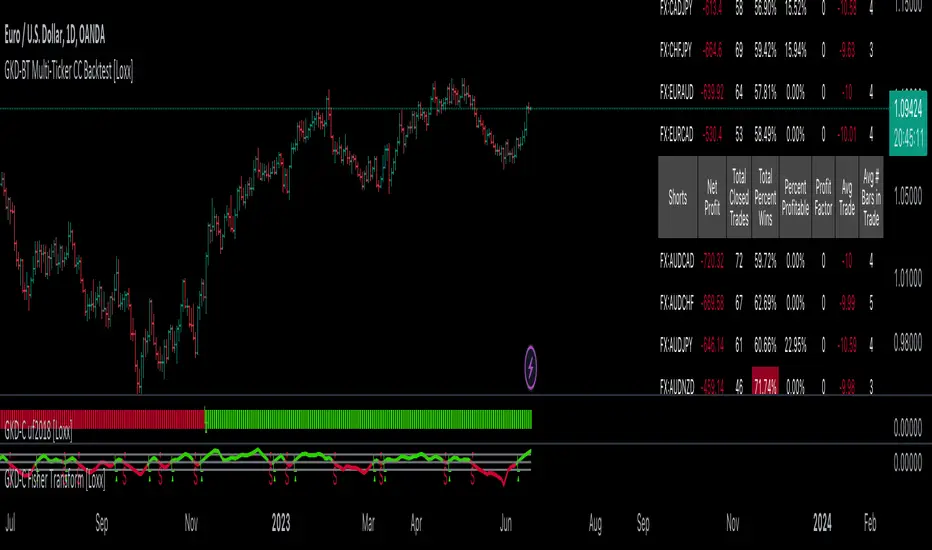
GKD-BT Optimizer SCC Backtest [Loxx]The Giga Kaleidoscope GKD-BT Optimizer SCC Backtest is a backtesting module included in Loxx's "Giga Kaleidoscope Modularized Trading System."
█ Giga Kaleidoscope GKD-BT Optimizer SCC Backtest
The Optimizer SCC Backtest is a Solo Confirmation Complex backtest that allows traders to test single GKD-C Confirmation indicator with GKD-B Baseline and GKD-V Volatility/Volume filtering across 10 varying inputs. The purpose of this backtest is to enable traders to optimize a GKD-C indicator given varying inputs.
The backtest module supports testing with 1 take profit and 1 stop loss. It also offers the option to limit testing to a specific date range, allowing simulated forward testing using historical data. This backtest module only includes standard long and short signals. Additionally, users can choose to display or hide a trading panel that provides relevant information about the backtest, statistics, and the current trade. Traders can also select a highlighting treshold for Total Percent Wins and Percent Profitable, and Profit Factor.
To use this indicator:
1. Import the value "Input into NEW GKD-BT Backtest" from the GKD-B Baseline indicator into the GKD-BT Optimizer SCC Backtest.
2. Import the value "Input into NEW GKD-BT Backtest" from the GKD-V Volatility/Volume indicator into the GKD-BT Optimizer SCC Backtest.
3. Select the "Optimizer" option in the GKD-C Confirmation indicator
4. Import a GKD-C indicator "Input into NEW GKD-BT Optimizer Backtest Signals" into the GKD-C Indicator Signals dropdown
5. Import a GKD-C indicator "Input into NEW GKD-BT Optimizer Backtest Start" into the GKD-C Indicator Start dropdown
6. Import a GKD-C indicator "Input into NEW GKD-BT Optimizer Backtest Skip" into the GKD-C Indicator Skip dropdown
This backtest includes the following metrics:
1. Net profit: Overall profit or loss achieved.
2. Total Closed Trades: Total number of closed trades, both winning and losing.
3. Total Percent Wins: Total wins, whether long or short, for the selected time interval regardless of commissions and other profit-modifying addons.
4. Percent Profitable: Total wins, whether long or short, that are also profitable, taking commissions into account.
5. Profit Factor: The ratio of gross profits to gross losses, indicating how much money the strategy made for every unit of money it lost.
6. Average Profit per Trade: The average gain or loss per trade, calculated by dividing the net profit by the total number of closed trades.
7. Average Number of Bars in Trade: The average number of bars that elapsed during trades for all closed trades.
Summary of notable settings:
Input Tickers separated by commas: Allows the user to input tickers separated by commas, specifying the symbols or tickers of financial instruments used in the backtest. The tickers should follow the format "EXCHANGE:TICKER" (e.g., "NASDAQ:AAPL, NYSE:MSFT").
Import GKD-B Baseline: Imports the "GKD-B Baseline" indicator.
Import GKD-V Volatility/Volume: Imports the "GKD-V Volatility/Volume" indicator.
Import GKD-C Confirmation: Imports the "GKD-C Confirmation" indicator.
Import GKD-C Continuation: Imports the "GKD-C Continuation" indicator.
Initial Capital: Represents the starting account balance for the backtest, denominated in the base currency of the trading account.
Order Size: Determines the quantity of contracts traded in each trade.
Order Type: Specifies the type of order used in the backtest, either "Contracts" or "% Equity."
Commission: Represents the commission per order or transaction cost incurred in each trade.
**the backtest data rendered to the chart above uses $5 commission per trade and 10% equity per trade with $1 million initial capital. Each backtest result for each ticker assumes these same inputs. The results are NOT cumulative, they are separate and isolate per ticker and trading side, long or short**
█ Volatility Types included
The GKD system utilizes volatility-based take profits and stop losses. Each take profit and stop loss is calculated as a multiple of volatility. You can change the values of the multipliers in the settings as well.
This module includes 17 types of volatility:
Close-to-Close
Parkinson
Garman-Klass
Rogers-Satchell
Yang-Zhang
Garman-Klass-Yang-Zhang
Exponential Weighted Moving Average
Standard Deviation of Log Returns
Pseudo GARCH(2,2)
Average True Range
True Range Double
Standard Deviation
Adaptive Deviation
Median Absolute Deviation
Efficiency-Ratio Adaptive ATR
Mean Absolute Deviation
Static Percent
Various volatility estimators and indicators that investors and traders can use to measure the dispersion or volatility of a financial instrument's price. Each estimator has its strengths and weaknesses, and the choice of estimator should depend on the specific needs and circumstances of the user.
Close-to-Close
Close-to-Close volatility is a classic and widely used volatility measure, sometimes referred to as historical volatility.
Volatility is an indicator of the speed of a stock price change. A stock with high volatility is one where the price changes rapidly and with a larger amplitude. The more volatile a stock is, the riskier it is.
Close-to-close historical volatility is calculated using only a stock's closing prices. It is the simplest volatility estimator. However, in many cases, it is not precise enough. Stock prices could jump significantly during a trading session and return to the opening value at the end. That means that a considerable amount of price information is not taken into account by close-to-close volatility.
Despite its drawbacks, Close-to-Close volatility is still useful in cases where the instrument doesn't have intraday prices. For example, mutual funds calculate their net asset values daily or weekly, and thus their prices are not suitable for more sophisticated volatility estimators.
Parkinson
Parkinson volatility is a volatility measure that uses the stock’s high and low price of the day.
The main difference between regular volatility and Parkinson volatility is that the latter uses high and low prices for a day, rather than only the closing price. This is useful as close-to-close prices could show little difference while large price movements could have occurred during the day. Thus, Parkinson's volatility is considered more precise and requires less data for calculation than close-to-close volatility.
One drawback of this estimator is that it doesn't take into account price movements after the market closes. Hence, it systematically undervalues volatility. This drawback is addressed in the Garman-Klass volatility estimator.
Garman-Klass
Garman-Klass is a volatility estimator that incorporates open, low, high, and close prices of a security.
Garman-Klass volatility extends Parkinson's volatility by taking into account the opening and closing prices. As markets are most active during the opening and closing of a trading session, it makes volatility estimation more accurate.
Garman and Klass also assumed that the process of price change follows a continuous diffusion process (Geometric Brownian motion). However, this assumption has several drawbacks. The method is not robust for opening jumps in price and trend movements.
Despite its drawbacks, the Garman-Klass estimator is still more effective than the basic formula since it takes into account not only the price at the beginning and end of the time interval but also intraday price extremes.
Researchers Rogers and Satchell have proposed a more efficient method for assessing historical volatility that takes into account price trends. See Rogers-Satchell Volatility for more detail.
Rogers-Satchell
Rogers-Satchell is an estimator for measuring the volatility of securities with an average return not equal to zero.
Unlike Parkinson and Garman-Klass estimators, Rogers-Satchell incorporates a drift term (mean return not equal to zero). As a result, it provides better volatility estimation when the underlying is trending.
The main disadvantage of this method is that it does not take into account price movements between trading sessions. This leads to an underestimation of volatility since price jumps periodically occur in the market precisely at the moments between sessions.
A more comprehensive estimator that also considers the gaps between sessions was developed based on the Rogers-Satchel formula in the 2000s by Yang-Zhang. See Yang Zhang Volatility for more detail.
Yang-Zhang
Yang Zhang is a historical volatility estimator that handles both opening jumps and the drift and has a minimum estimation error.
Yang-Zhang volatility can be thought of as a combination of the overnight (close-to-open volatility) and a weighted average of the Rogers-Satchell volatility and the day’s open-to-close volatility. It is considered to be 14 times more efficient than the close-to-close estimator.
Garman-Klass-Yang-Zhang
Garman-Klass-Yang-Zhang (GKYZ) volatility estimator incorporates the returns of open, high, low, and closing prices in its calculation.
GKYZ volatility estimator takes into account overnight jumps but not the trend, i.e., it assumes that the underlying asset follows a Geometric Brownian Motion (GBM) process with zero drift. Therefore, the GKYZ volatility estimator tends to overestimate the volatility when the drift is different from zero. However, for a GBM process, this estimator is eight times more efficient than the close-to-close volatility estimator.
Exponential Weighted Moving Average
The Exponentially Weighted Moving Average (EWMA) is a quantitative or statistical measure used to model or describe a time series. The EWMA is widely used in finance, with the main applications being technical analysis and volatility modeling.
The moving average is designed such that older observations are given lower weights. The weights decrease exponentially as the data point gets older – hence the name exponentially weighted.
The only decision a user of the EWMA must make is the parameter lambda. The parameter decides how important the current observation is in the calculation of the EWMA. The higher the value of lambda, the more closely the EWMA tracks the original time series.
Standard Deviation of Log Returns
This is the simplest calculation of volatility. It's the standard deviation of ln(close/close(1)).
Pseudo GARCH(2,2)
This is calculated using a short- and long-run mean of variance multiplied by ?.
?avg(var;M) + (1 ? ?) avg(var;N) = 2?var/(M+1-(M-1)L) + 2(1-?)var/(M+1-(M-1)L)
Solving for ? can be done by minimizing the mean squared error of estimation; that is, regressing L^-1var - avg(var; N) against avg(var; M) - avg(var; N) and using the resulting beta estimate as ?.
Average True Range
The average true range (ATR) is a technical analysis indicator, introduced by market technician J. Welles Wilder Jr. in his book New Concepts in Technical Trading Systems, that measures market volatility by decomposing the entire range of an asset price for that period.
The true range indicator is taken as the greatest of the following: current high less the current low; the absolute value of the current high less the previous close; and the absolute value of the current low less the previous close. The ATR is then a moving average, generally using 14 days, of the true ranges.
True Range Double
A special case of ATR that attempts to correct for volatility skew.
Standard Deviation
Standard deviation is a statistic that measures the dispersion of a dataset relative to its mean and is calculated as the square root of the variance. The standard deviation is calculated as the square root of variance by determining each data point's deviation relative to the mean. If the data points are further from the mean, there is a higher deviation within the data set; thus, the more spread out the data, the higher the standard deviation.
Adaptive Deviation
By definition, the Standard Deviation (STD, also represented by the Greek letter sigma ? or the Latin letter s) is a measure that is used to quantify the amount of variation or dispersion of a set of data values. In technical analysis, we usually use it to measure the level of current volatility.
Standard Deviation is based on Simple Moving Average calculation for mean value. This version of standard deviation uses the properties of EMA to calculate what can be called a new type of deviation, and since it is based on EMA, we can call it EMA deviation. Additionally, Perry Kaufman's efficiency ratio is used to make it adaptive (since all EMA type calculations are nearly perfect for adapting).
The difference when compared to the standard is significant--not just because of EMA usage, but the efficiency ratio makes it a "bit more logical" in very volatile market conditions.
Median Absolute Deviation
The median absolute deviation is a measure of statistical dispersion. Moreover, the MAD is a robust statistic, being more resilient to outliers in a data set than the standard deviation. In the standard deviation, the distances from the mean are squared, so large deviations are weighted more heavily, and thus outliers can heavily influence it. In the MAD, the deviations of a small number of outliers are irrelevant.
Because the MAD is a more robust estimator of scale than the sample variance or standard deviation, it works better with distributions without a mean or variance, such as the Cauchy distribution.
For this indicator, a manual recreation of the quantile function in Pine Script is used. This is so users have a full inside view into how this is calculated.
Efficiency-Ratio Adaptive ATR
Average True Range (ATR) is a widely used indicator for many occasions in technical analysis. It is calculated as the RMA of the true range. This version adds a "twist": it uses Perry Kaufman's Efficiency Ratio to calculate adaptive true range.
Mean Absolute Deviation
The mean absolute deviation (MAD) is a measure of variability that indicates the average distance between observations and their mean. MAD uses the original units of the data, which simplifies interpretation. Larger values signify that the data points spread out further from the average. Conversely, lower values correspond to data points bunching closer to it. The mean absolute deviation is also known as the mean deviation and average absolute deviation.
This definition of the mean absolute deviation sounds similar to the standard deviation (SD). While both measure variability, they have different calculations. In recent years, some proponents of MAD have suggested that it replace the SD as the primary measure because it is a simpler concept that better fits real life.
█ Giga Kaleidoscope Modularized Trading System
Core components of an NNFX algorithmic trading strategy
The NNFX algorithm is built on the principles of trend, momentum, and volatility. There are six core components in the NNFX trading algorithm:
1. Volatility - price volatility; e.g., Average True Range, True Range Double, Close-to-Close, etc.
2. Baseline - a moving average to identify price trend
3. Confirmation 1 - a technical indicator used to identify trends
4. Confirmation 2 - a technical indicator used to identify trends
5. Continuation - a technical indicator used to identify trends
6. Volatility/Volume - a technical indicator used to identify volatility/volume breakouts/breakdown
7. Exit - a technical indicator used to determine when a trend is exhausted
8. Metamorphosis - a technical indicator that produces a compound signal from the combination of other GKD indicators*
*(not part of the NNFX algorithm)
What is Volatility in the NNFX trading system?
In the NNFX (No Nonsense Forex) trading system, ATR (Average True Range) is typically used to measure the volatility of an asset. It is used as a part of the system to help determine the appropriate stop loss and take profit levels for a trade. ATR is calculated by taking the average of the true range values over a specified period.
True range is calculated as the maximum of the following values:
-Current high minus the current low
-Absolute value of the current high minus the previous close
-Absolute value of the current low minus the previous close
ATR is a dynamic indicator that changes with changes in volatility. As volatility increases, the value of ATR increases, and as volatility decreases, the value of ATR decreases. By using ATR in NNFX system, traders can adjust their stop loss and take profit levels according to the volatility of the asset being traded. This helps to ensure that the trade is given enough room to move, while also minimizing potential losses.
Other types of volatility include True Range Double (TRD), Close-to-Close, and Garman-Klass
What is a Baseline indicator?
The baseline is essentially a moving average, and is used to determine the overall direction of the market.
The baseline in the NNFX system is used to filter out trades that are not in line with the long-term trend of the market. The baseline is plotted on the chart along with other indicators, such as the Moving Average (MA), the Relative Strength Index (RSI), and the Average True Range (ATR).
Trades are only taken when the price is in the same direction as the baseline. For example, if the baseline is sloping upwards, only long trades are taken, and if the baseline is sloping downwards, only short trades are taken. This approach helps to ensure that trades are in line with the overall trend of the market, and reduces the risk of entering trades that are likely to fail.
By using a baseline in the NNFX system, traders can have a clear reference point for determining the overall trend of the market, and can make more informed trading decisions. The baseline helps to filter out noise and false signals, and ensures that trades are taken in the direction of the long-term trend.
What is a Confirmation indicator?
Confirmation indicators are technical indicators that are used to confirm the signals generated by primary indicators. Primary indicators are the core indicators used in the NNFX system, such as the Average True Range (ATR), the Moving Average (MA), and the Relative Strength Index (RSI).
The purpose of the confirmation indicators is to reduce false signals and improve the accuracy of the trading system. They are designed to confirm the signals generated by the primary indicators by providing additional information about the strength and direction of the trend.
Some examples of confirmation indicators that may be used in the NNFX system include the Bollinger Bands, the MACD (Moving Average Convergence Divergence), and the MACD Oscillator. These indicators can provide information about the volatility, momentum, and trend strength of the market, and can be used to confirm the signals generated by the primary indicators.
In the NNFX system, confirmation indicators are used in combination with primary indicators and other filters to create a trading system that is robust and reliable. By using multiple indicators to confirm trading signals, the system aims to reduce the risk of false signals and improve the overall profitability of the trades.
What is a Continuation indicator?
In the NNFX (No Nonsense Forex) trading system, a continuation indicator is a technical indicator that is used to confirm a current trend and predict that the trend is likely to continue in the same direction. A continuation indicator is typically used in conjunction with other indicators in the system, such as a baseline indicator, to provide a comprehensive trading strategy.
What is a Volatility/Volume indicator?
Volume indicators, such as the On Balance Volume (OBV), the Chaikin Money Flow (CMF), or the Volume Price Trend (VPT), are used to measure the amount of buying and selling activity in a market. They are based on the trading volume of the market, and can provide information about the strength of the trend. In the NNFX system, volume indicators are used to confirm trading signals generated by the Moving Average and the Relative Strength Index. Volatility indicators include Average Direction Index, Waddah Attar, and Volatility Ratio. In the NNFX trading system, volatility is a proxy for volume and vice versa.
By using volume indicators as confirmation tools, the NNFX trading system aims to reduce the risk of false signals and improve the overall profitability of trades. These indicators can provide additional information about the market that is not captured by the primary indicators, and can help traders to make more informed trading decisions. In addition, volume indicators can be used to identify potential changes in market trends and to confirm the strength of price movements.
What is an Exit indicator?
The exit indicator is used in conjunction with other indicators in the system, such as the Moving Average (MA), the Relative Strength Index (RSI), and the Average True Range (ATR), to provide a comprehensive trading strategy.
The exit indicator in the NNFX system can be any technical indicator that is deemed effective at identifying optimal exit points. Examples of exit indicators that are commonly used include the Parabolic SAR, the Average Directional Index (ADX), and the Chandelier Exit.
The purpose of the exit indicator is to identify when a trend is likely to reverse or when the market conditions have changed, signaling the need to exit a trade. By using an exit indicator, traders can manage their risk and prevent significant losses.
In the NNFX system, the exit indicator is used in conjunction with a stop loss and a take profit order to maximize profits and minimize losses. The stop loss order is used to limit the amount of loss that can be incurred if the trade goes against the trader, while the take profit order is used to lock in profits when the trade is moving in the trader's favor.
Overall, the use of an exit indicator in the NNFX trading system is an important component of a comprehensive trading strategy. It allows traders to manage their risk effectively and improve the profitability of their trades by exiting at the right time.
What is an Metamorphosis indicator?
The concept of a metamorphosis indicator involves the integration of two or more GKD indicators to generate a compound signal. This is achieved by evaluating the accuracy of each indicator and selecting the signal from the indicator with the highest accuracy. As an illustration, let's consider a scenario where we calculate the accuracy of 10 indicators and choose the signal from the indicator that demonstrates the highest accuracy.
The resulting output from the metamorphosis indicator can then be utilized in a GKD-BT backtest by occupying a slot that aligns with the purpose of the metamorphosis indicator. The slot can be a GKD-B, GKD-C, or GKD-E slot, depending on the specific requirements and objectives of the indicator. This allows for seamless integration and utilization of the compound signal within the GKD-BT framework.
How does Loxx's GKD (Giga Kaleidoscope Modularized Trading System) implement the NNFX algorithm outlined above?
Loxx's GKD v2.0 system has five types of modules (indicators/strategies). These modules are:
1. GKD-BT - Backtesting module (Volatility, Number 1 in the NNFX algorithm)
2. GKD-B - Baseline module (Baseline and Volatility/Volume, Numbers 1 and 2 in the NNFX algorithm)
3. GKD-C - Confirmation 1/2 and Continuation module (Confirmation 1/2 and Continuation, Numbers 3, 4, and 5 in the NNFX algorithm)
4. GKD-V - Volatility/Volume module (Confirmation 1/2, Number 6 in the NNFX algorithm)
5. GKD-E - Exit module (Exit, Number 7 in the NNFX algorithm)
6. GKD-M - Metamorphosis module (Metamorphosis, Number 8 in the NNFX algorithm, but not part of the NNFX algorithm)
(additional module types will added in future releases)
Each module interacts with every module by passing data to A backtest module wherein the various components of the GKD system are combined to create a trading signal.
That is, the Baseline indicator passes its data to Volatility/Volume. The Volatility/Volume indicator passes its values to the Confirmation 1 indicator. The Confirmation 1 indicator passes its values to the Confirmation 2 indicator. The Confirmation 2 indicator passes its values to the Continuation indicator. The Continuation indicator passes its values to the Exit indicator, and finally, the Exit indicator passes its values to the Backtest strategy.
This chaining of indicators requires that each module conform to Loxx's GKD protocol, therefore allowing for the testing of every possible combination of technical indicators that make up the six components of the NNFX algorithm.
What does the application of the GKD trading system look like?
Example trading system:
Backtest: Optimizer Full GKD Backtest as shown on the chart above
Baseline: Hull Moving Average
Volatility/Volume: Hurst Exponent
Confirmation 1: Fisher Transofrm as shown on the chart above
Confirmation 2: uf2018
Continuation: Coppock Curve
Exit: Rex Oscillator
Metamorphosis: Baseline Optimizer
Each GKD indicator is denoted with a module identifier of either: GKD-BT, GKD-B, GKD-C, GKD-V, GKD-M, or GKD-E. This allows traders to understand to which module each indicator belongs and where each indicator fits into the GKD system.
█ Giga Kaleidoscope Modularized Trading System Signals
Standard Entry
1. GKD-C Confirmation gives signal
2. Baseline agrees
3. Price inside Goldie Locks Zone Minimum
4. Price inside Goldie Locks Zone Maximum
5. Confirmation 2 agrees
6. Volatility/Volume agrees
1-Candle Standard Entry
1a. GKD-C Confirmation gives signal
2a. Baseline agrees
3a. Price inside Goldie Locks Zone Minimum
4a. Price inside Goldie Locks Zone Maximum
Next Candle
1b. Price retraced
2b. Baseline agrees
3b. Confirmation 1 agrees
4b. Confirmation 2 agrees
5b. Volatility/Volume agrees
Baseline Entry
1. GKD-B Baseline gives signal
2. Confirmation 1 agrees
3. Price inside Goldie Locks Zone Minimum
4. Price inside Goldie Locks Zone Maximum
5. Confirmation 2 agrees
6. Volatility/Volume agrees
7. Confirmation 1 signal was less than 'Maximum Allowable PSBC Bars Back' prior
1-Candle Baseline Entry
1a. GKD-B Baseline gives signal
2a. Confirmation 1 agrees
3a. Price inside Goldie Locks Zone Minimum
4a. Price inside Goldie Locks Zone Maximum
5a. Confirmation 1 signal was less than 'Maximum Allowable PSBC Bars Back' prior
Next Candle
1b. Price retraced
2b. Baseline agrees
3b. Confirmation 1 agrees
4b. Confirmation 2 agrees
5b. Volatility/Volume agrees
Volatility/Volume Entry
1. GKD-V Volatility/Volume gives signal
2. Confirmation 1 agrees
3. Price inside Goldie Locks Zone Minimum
4. Price inside Goldie Locks Zone Maximum
5. Confirmation 2 agrees
6. Baseline agrees
7. Confirmation 1 signal was less than 7 candles prior
1-Candle Volatility/Volume Entry
1a. GKD-V Volatility/Volume gives signal
2a. Confirmation 1 agrees
3a. Price inside Goldie Locks Zone Minimum
4a. Price inside Goldie Locks Zone Maximum
5a. Confirmation 1 signal was less than 'Maximum Allowable PSVVC Bars Back' prior
Next Candle
1b. Price retraced
2b. Volatility/Volume agrees
3b. Confirmation 1 agrees
4b. Confirmation 2 agrees
5b. Baseline agrees
Confirmation 2 Entry
1. GKD-C Confirmation 2 gives signal
2. Confirmation 1 agrees
3. Price inside Goldie Locks Zone Minimum
4. Price inside Goldie Locks Zone Maximum
5. Volatility/Volume agrees
6. Baseline agrees
7. Confirmation 1 signal was less than 7 candles prior
1-Candle Confirmation 2 Entry
1a. GKD-C Confirmation 2 gives signal
2a. Confirmation 1 agrees
3a. Price inside Goldie Locks Zone Minimum
4a. Price inside Goldie Locks Zone Maximum
5a. Confirmation 1 signal was less than 'Maximum Allowable PSC2C Bars Back' prior
Next Candle
1b. Price retraced
2b. Confirmation 2 agrees
3b. Confirmation 1 agrees
4b. Volatility/Volume agrees
5b. Baseline agrees
PullBack Entry
1a. GKD-B Baseline gives signal
2a. Confirmation 1 agrees
3a. Price is beyond 1.0x Volatility of Baseline
Next Candle
1b. Price inside Goldie Locks Zone Minimum
2b. Price inside Goldie Locks Zone Maximum
3b. Confirmation 1 agrees
4b. Confirmation 2 agrees
5b. Volatility/Volume agrees
Continuation Entry
1. Standard Entry, 1-Candle Standard Entry, Baseline Entry, 1-Candle Baseline Entry, Volatility/Volume Entry, 1-Candle Volatility/Volume Entry, Confirmation 2 Entry, 1-Candle Confirmation 2 Entry, or Pullback entry triggered previously
2. Baseline hasn't crossed since entry signal trigger
4. Confirmation 1 agrees
5. Baseline agrees
6. Confirmation 2 agrees
█ Connecting to Backtests
All GKD indicators are chained indicators meaning you export the value of the indicators to specialized backtest to creat your GKD trading system. Each indicator contains a proprietary signal generation algo that will only work with GKD backtests. You can find these backtests using the links below.
GKD-BT Giga Confirmation Stack Backtest
GKD-BT Giga Stacks Backtest
GKD-BT Full Giga Kaleidoscope Backtest
GKD-BT Solo Confirmation Super Complex Backtest
GKD-BT Solo Confirmation Complex Backtest
GKD-BT Solo Confirmation Simple Backtest
GKD-M Baseline Optimizer
GKD-M Accuracy Alchemist
GKD-BT Optimizer SCC Backtest
GKD-BT Optimizer SCC Backtest
GKD-BT Optimizer SCC Backtest
GKD-C GKD-BT Optimizer Full GKD Backtest