AQPRO ScalperX📝 INTRODUCTION
AQPRO ScalperX is a trading indicator designed for fast-paced, intraday trading. It uses Donchian channel breakouts, combined with a proprietary filtering system, to catch buy and sell opportunities as close to the beginning as possible without losing quality of the signals.
On top of core signals, ScalperX includes a real-time max profit tracker, a multi-timeframe (MTF) dashboard, support and resistance zones, and risk management visualization tools like automatic rendering of TP and SL lines. The indicator is fully customizable for both its visuals and functional settings.
🎯 PURPOSE OF USAGE
This indicator was initially designed with the idea of trying to make such a tool, that would be able to catch trend reversal in the most safe way. In this particular situation term 'safe way' is very abstract and it is up to interpretation, but we decided that our definition will be 'trading with price breakouts' , meaning that we would like to capitalize on price breaking its previous structure in the direction opposite to the previous one.
You can clearly see on the chart how buy and sell signals are going one after another on the screenshot below:
This ensures that we follow trend consistently and without missing out on potential profits. Just like they say: " let the winners run ".
Even though indicator with similar goals already exist in the open market, we believe that our proprietary algorithms and filters for determining price breakouts can make a big difference to traders, which employ similar strategies on daily basis, by helping them understand where are the potential high-quality breakouts might be. We haven't found indicator with exact same functionality as ours, which means that traders will be able to leverage an actually new tool to generate new price insights.
In short, main goals of this indicator are as follows:
Catching high-quality price breakouts, filtered to reduce the amount of choppy moves and false signals;
Tracking potential profits in real-time, directly on trader's chart;
Organizing data visualization of data pf latest signals from chosen asset from multiple timeframe in one dashboard;
Automated highlighting of key support and resistance zones on the chart, which serve as confirmation for main signals;
⚙️ SETTINGS OVERVIEW
Options for customization of this indicator are straightforward, but let's review them to make things certainly clear:
🔑 ScalperX / Main Settings
Range — defines the "wideness" of the breakout boxes. Higher values create wider breakout zones and impact breakout sensitivity;
Filter — adjusts the spacing between breakout boxes, determining the strictness of signal filtering. Higher values lead to more selective and rarer signals;
Show Max Profit — displays a real-time line and label that updates when a trade achieves a new peak profit, measured in ticks.
⏰ MTF Signal / Main Settings
Show MTF Signals — enables the generation of buy/sell signals from selected higher timeframes, displayed as labels on the current chart;
Timeframe — specifies the higher timeframe to use for MTF signal detection, such as 1 hour (1h) or 4 hours (4h).
🗂️ MTF Dashboard / Main Settings
Show MTF Dashboard — activates a dashboard that tracks entries, TP, SL, and overall trade bias for one selected symbol across four customizable timeframes;
* Dashboard position ( Vertical ) — adjusts whether the dashboard appears on the Top, Middle, or Bottom of the chart;
* Dashboard position ( Horizontal ) — aligns the dashboard Left, Center, or Right within the chart window;
* the name of the parameter is hidden in the settings
🗂️ MTF Dashboard / Ticker
Ticker to Track — Allows you to choose the specific ticker symbol (e.g., BINANCE:BTCUSDT) for MTF tracking.
🗂️ MTF Dashboard / Timeframes
* Timeframe 1 — set the first timeframe for multi-timeframe analysis (e.g., 15 minutes);
* Timeframe 2 — set the second timeframe for multi-timeframe analysis (e.g., 30 minutes);
* Timeframe 3 — set the third timeframe for multi-timeframe analysis (e.g., 1 hour);
* Timeframe 4 — set the fourth timeframe for multi-timeframe analysis (e.g., 4 hours).
* the name of the parameter is hidden in the settings
🛡️ Risk Management / Main Settings
Show TP&SL — displays dynamic lines and labels for the entry, Take Profit (TP), and Stop Loss (SL) of the most recent signal, updated in real-time until a new signal triggers;
Risk-to-Reward Ratio (R:R) — defines the ratio for TP and SL calculation to control your risk and reward on every trade.
📐 Support & Resistance / Main Settings
Show Support & Resistance Zones — enables dynamic zones based on pivot points, colored bullish or bearish based on price context;
History Lookback — defines the number of bars to consider when calculating support and resistance levels. Increasing this results in zones derived from longer-term price structures.
🎨 Visual Settings / ScalperX
Bullish Box — defines the color for bullish breakout boxes;
Bearish Box — defines the color for bearish breakout boxes;
Max Profit — sets the color for the max profit line on the chart.
🎨 Visual Settings / S&R
Support — defines color used for standard support zones;
Resistance — defines color used for standard resistance zones;
Strong Support — defines special color for zones classified as "strong support";
Strong Resistance — defines special color for zones classified as "strong resistance".
🎨 Visual Settings / MTF Dashboard
Bullish — sets the color for bullish trade states in the MTF dashboard;
Bearish — sets the color for bearish trade states in the MTF dashboard.
🔔 Alerts / Main Settings
Buy & Sell — toggles alerts for buy and sell signals detected by the indicator in the current chart timeframe;
MTF Buy & Sell — toggles alerts for buy and sell signals detected across the selected MTF timeframes.
📈 APPLICATION GUIDE
Application flow of this indicator very easy to understand and get used to, because all of the necessary elements — analysis, drawing, alert — are already automated by our algorithms. Let's review how the indicator works.
Let's start with the most basic thing — how will your indicator look when you load it on your chart for the first time:
AQPRO ScalperX consists mainly of 6 logic blocks:
ScalperX signals;
Risk visualization;
Max Profit tracking;
MTF scalper signals;
MTF dashboard;
Support & Resistance zones.
Description of each logic block is provided in the corresponding sections below.
SCALPERX SIGNALS
Signals, generated by our indicator, are shown on the chart as coloured up/down triangle. When a signal appears on the chart, indicator also create a box of length equal to 'Range' parameter from "Main Settings" group of settings. This box is intended to show which area of the price was broken by current candle.
It also important to acknowledge, the breakout itself happens only when price closes beyond broken price area with its close (!) price . Breakouts with highs or lows are not counted. This reduces the amount of low-quality signals and ensures that only the strong breakout will appear on the chart.
VERY IMPORTANT NOTE: all signals are considered valid only on the close of the candle, which triggered the signal, so if you want to enter a trade by any signal, wait for its candle to close and open your trade right on the next candle.
Talking about scalper's settings, we need to shed a light on how the changes in them affect signal's quality.
Parameter 'Range' defines the amount of bars, that will be review prior to current candle to determine wether the price area of this bars is good enough to track and if current candle actually broke this price area.
👍 Rule of thumb : the higher the 'Range' is, the "wider" the boxes. Also the with the increase of this parameter rises the lag of the signals, so be carefully with setting high values to this parameter.
See the visual showcase of signals with different 'Range' parameters on the screenshot below:
The example above features two instancies of ScalperX with two different 'Range' parameter values: 15 (leftchart) and 5 (right chart). You can clearly see, that on left chart here are 2 signals in comparison to 6 signals on right chart. Also signals on the left side have bigger lag and they don't catch the start of the move in comparison to how quickly tops and bottoms are catched with low 'Range' . However, low 'Range' will lead to excessive amount of signals, quality of which during 'whipsaw' markets is not that great.
✉️ Our advice on how to optimally set 'Range' parameter:
Use low values to trade during the times, when there are a lot of clean up and down impulses. This way you will catch reversal opportunities sooner and the quality of the signals will still be great;
Use high values on the 'whipsaw' markets. This will filter out many bad signals, that you would get with low-value 'Range' , and will drastically reduces amount of losing trades.
Talking about the 'Filter' parameter, this particular setting defines the 'strictness' of rules which will be applied to price area validation process. Essentially, the higher this parameter is, the stronger price impulse has to be confirm the breakout. However, changes in this parameter will not impact the "wideness" of boxes at all.
👍 Rule of thumb : the higher the 'Filter' is, the more separated the signal will be. Setting this parameter to high value will lead to increase in lag and big reduction in amount of signals, so be careful this parameter to high values.
See the visual showcase of signals with different 'Filter' parameters on the screenshot below:
The example above features two instancies of ScalperX with two different 'Filter' parameter values: 20 (left chart) and 2.5 (right chart). You can clear see, that low 'Filter' generated 6 signals, while higher one generated only 4 signals. However if you look closer, you will see that 2 signals, that existing in the yellow dashed area on the right chart, don't exist in the same area on the left chart. This is because high value of this parameter requires price impulse to be very strong in order for the indicator to mark this breakout as a valid one. What is more important is that these 2 'missing' signals were actually bad and, technically, we actually cut our losses in this case with high value of 'Filter' . You can see that the leftmost sell signal on the left chart eventually closed in a nice profit, in comparison to the same trade being closed in a loss on the right chart because of the 2 signals that we were talking about above.
It is important to note, that setting 'Filter' to low values will not affect performance this much as it low value of 'Range' do, because the indicator already works on low values of this parameter by default and the signals on average are already good enough for trading.
✉️ Our advice on how to optimally set 'Filter' parameter:
Use low values to trade on the markets with clean up and down impulses. This way you avoid excessive filtering and leave a room for good signals to come right at you;
Use high values to trade on 'whipsaw' markets. Higher values of this parameter on these markets have same effect as high 'Range' parameter: filtering false signals and leaving room for actually strong price impulses, which you will later capitalize on.
RISK VISUALIZATION (TP&SL)
Rendering Take-Profits and Stop-Losses in our indicator works quite simple: for each new trade indicator creates new pairs of lines and labels for TP and SL, while lines & labels from previous trade are erased for aesthetics purposes. Each label shows price coordinates, so that each trader would be able to grap the numbers in seconds.
See the visual showcase of TP & SL visualization on the screenshot below:
Also, whenever TP or SL of the current trade is reached, drawing of both TP and SL stops. When the TP is reached, additional '✅' emoji on the TP price is shown as confirmation of Take-Profit.
However, while TP or SL has not been reached, TP&SL labels and lines will be prolonged until one of them will be reached or new signals will come.
See the visual showcase of TP & SL stopping being visualized & TP on the screenshot below:
MAX PROFIT TRACKING
This mechanic is not particularly a new one in field of trading, but people usually forgot that it can be a useful indicator of state of the market:
when lines and labels of Max Profit are far from entry points on consistent basis , it usually means that indicator's signals actually can catch a beginning of good price moves, which enables trader to capitalize on them;
when lines and labels of Max Profit are close to entry points on consistent basis , it means that either market is choppy or the indicator can't catch trading opportunities in time. To 'fix' this you can try to reconfigure scalper's parameters, which were described above.
Principles of Max Profit in this indicator are of industry-standard: when price updates its extremum and 'generates' more profit than it previously did, Max Profit label and line change their position to this extremum. Max Profit label displays the maximum potential amount of profit that a trader could have got during this trade in pips (!) .
See the visual showcase of Max Profit work on the screenshot below:
MTF SCALPER SIGNALS
The principles of these signals are exactly the same as principles for classic Scalper signals. Refer to 'Scalper Signals' section above to rehearse the knowledge.
Logic behind these signals is very simple:
We take classic Scalper signals;
We request the data about these latest signals from specific other timeframe ( user can choose it in the settings );
If such signals appeared, we display it on the chart as a big label with timeframe value inside of it. In comparison to classic signals, no additional boxes are created . TP&SL functionality doesn't cover MTF signals, so don't expect to see TP&SL lines and labels for MTF signals.
See the visual showcase of MTF Scalper signals on the screenshot below:
MTF DASHBOARD
The functionality of the dashboard is pretty simple, but it makes the dashboard itself a very powerful tool in a hands of experienced trader.
Let's review structure of MTF dashboard on the screenshot below:
The important feature of MTF dashboard is that its tracks latest trade's data from a particular ticker and its four timeframes, all of which any trader chooses in the settings. This means, that you can be on asset ABC , but track the data from asset XYZ . This allows for a quick scan of sentiment from different assets and their timeframes, which gives traders a clue on what is the trend on these assets both on lower and higher timeframes at the same moment and saves a lot of time from jumping from one asset & timeframe to another.
To see that this is exactly the case with our indicator, see the screenshot below:
Needless to say, that you can track current asset in the dashboard as well. This will have the same benefits, described in the paragraph above.
You can also customize colours for bullish and bearish patterns for MTF Dashboard in the settings.
SUPPORT & RESISTANCE ZONES
Support & resistance (S&R) zones are a great tool for confirming Scalper signals in complex situations. Using these zones to determine whether or a particular entry opportunity is good is a practice of professional traders, which we specifically added to our indicator for the reason of improving the quality of Scalper signals in long run.
The mechanics behind these zones is based on pivot points, the lookback for which you can customize in the parameter called 'History Lookback (Bars)' in "Support & Resistance / Main Settings" group of settings. Increasing this parameter will lead to a appearance of more 'global' zones, but they will appear much rarer, rather then zones, generated with low values of this parameter.
The quality of these zones doesn't change much when changing this parameter — it only changes the frequency of the zones on the chart. Zones, generated from high values of this parameter are more suitable for long-term trading, while zones, generated from low value of this parameter, are more suitable for short-term trading.
It also important to mention that any zone on the chart is considered active only until the moment its farther border ( top border for resistance zones and bottom border for support zones) is reached by price's high or low .
Take a look on the screenshot below to see which zones does the indicator draw:
Let's review the zones themselves now:
Classic Support/Resistance Zone — a standard zone, which on average has amedium success rate to reverse the price when collided with it;
High-buyer-volume/High-seller-volume Support/Resistance Zone — a stronger zone, which on average has much better success rate to reverse the price when collided with it. Classic zone is marked as high-volume only if the up/down volume near the pivot point of this zone is greater than a certain threshold ( not changeable );
Extreme Support/Resistance Zone — a zone, which appeared beyond price's least-possible-to-cross levels, and has to the highest success rate of reversing the price on encounter across the zones, mentioned previously. Classic zone, which appeared beyond certain price levels, calculated with our proprietary risk system, is considered extreme. Classic zone doesn't need to be high-volume to become an Extreme Zone!
High-buyer-volume/High-seller-volume Extreme Support/Resistance Zone — an Extreme Zone, which has also passed up/down volume evolution process, mentioned in the point 2 .
Trading with the zones, mentioned above, with highest-on-paper success rate — especially Extreme Zones — does NOT guarantee you a price reversal when the price will reach this zone. However, by conducting our own extensive research with this indicator, we have found that using these zone will actually help you increase your success rate on average, because using these zones as confirmation systems filter out quite a number of false signals on average.
It is also important to mention, that opacity (same as 'transparency') of S&R zones depends on the volume of around zone's pivot point:
if volume is high , zone has 'brighter' (less opacity) colour;
if volume is low , zone has 'darker' (more opacity) colour.
Let's review examples of Scalper signal, which 1) where filtered out by our S&R zones and 2) where confirmed by our S&R zones. See the screenshot below:
The example above clearly shows the importance of having an S&R zone confirming the signal. This kind of 'team work' between of Scalper signals and S&R zones results in filtering lots of bad signals and confirmation of truly strong ones.
🔔 ALERTS
This indicator employs alerts for an event when new signal occurs on the current timeframe or on MTF timeframe. While creating the alert below 'Condition' field choose 'any alert() function call'.
When this alert is triggered, it will generate this kind of message:
// Alerts for current timeframe
string msg_template = "EXCHANGE:ASSET, TIMEFRAME: BUY_OR_SELL"
string msg_example = "BINANCE:BTCUSDT, 15m: Buy"
// Alerts for MTF timeframe
string msg_template_mtf = "MTF / EXCHANGE:ASSET, TIMEFRAME: BUY_OR_SELL"
string msg_example_mtf = "MTF / BINANCE:BTCUSDT, 1h: Buy"
📌 NOTES
This indicators works best on assets with high liquidity; most suitable timeframes range from 1m to 4h (depends on your trading style) ;
Seriously consider using S&R zones as confirmation to main Scalper signals or any of your own signals. Confirmation process may filter out a lot of signals, but your PNL History will say "thank you" to you in the long-run and you will see yourself how good confirmed signals actually do work;
Don't forget to look at MTF dashboard from time to time to see global sentiment. This will help you time your entry moments better and will improve your performance in the long run;
This indicator can serve both as primary source of signals and as confirmation tool, but we advise to try to combine it with your own strategy frst to see if it will improve your performance.
🏁 AFTERWORD
AQPRO ScalperX was designed to help traders identify high-quality price breakouts and generate market insights based on them, which include signal generation. Main feature of this indicator is Scalper algorithm, which generate price-breakout-based signals directly on your chart.
Alongside these signals you can leverage 1) MTF Dashboard to track latest trade's data from chosen asset and its four timeframes, 2) risk visualization functionality (TP&SL) to improve understanding of current market risks and 3) Support & Resistance zones, which serve as a great confirmation tool for Scalper signals, but can also work with any other signal generation tool to enhance its performance.
ℹ️ If you have questions about this or any other our indicator, please leave it in the comments.
Cari dalam skrip untuk "profit"

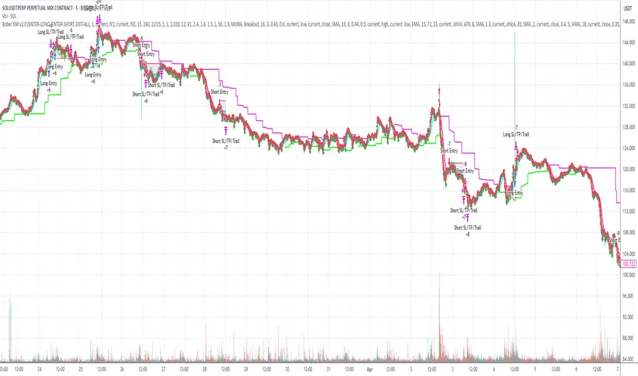
Bober XM v2.0# ₿ober XM v2.0 Trading Bot Documentation
**Developer's Note**: While our previous Bot 1.3.1 was removed due to guideline violations, this setback only fueled our determination to create something even better. Rising from this challenge, Bober XM 2.0 emerges not just as an update, but as a complete reimagining with multi-timeframe analysis, enhanced filters, and superior adaptability. This adversity pushed us to innovate further and deliver a strategy that's smarter, more agile, and more powerful than ever before. Challenges create opportunity - welcome to Cryptobeat's finest work yet.
## !!!!You need to tune it for your own pair and timeframe and retune it periodicaly!!!!!
## Overview
The ₿ober XM v2.0 is an advanced dual-channel trading bot with multi-timeframe analysis capabilities. It integrates multiple technical indicators, customizable risk management, and advanced order execution via webhook for automated trading. The bot's distinctive feature is its separate channel systems for long and short positions, allowing for asymmetric trade strategies that adapt to different market conditions across multiple timeframes.
### Key Features
- **Multi-Timeframe Analysis**: Analyze price data across multiple timeframes simultaneously
- **Dual Channel System**: Separate parameter sets for long and short positions
- **Advanced Entry Filters**: RSI, Volatility, Volume, Bollinger Bands, and KEMAD filters
- **Machine Learning Moving Average**: Adaptive prediction-based channels
- **Multiple Entry Strategies**: Breakout, Pullback, and Mean Reversion modes
- **Risk Management**: Customizable stop-loss, take-profit, and trailing stop settings
- **Webhook Integration**: Compatible with external trading bots and platforms
### Strategy Components
| Component | Description |
|---------|-------------|
| **Dual Channel Trading** | Uses either Keltner Channels or Machine Learning Moving Average (MLMA) with separate settings for long and short positions |
| **MLMA Implementation** | Machine learning algorithm that predicts future price movements and creates adaptive bands |
| **Pivot Point SuperTrend** | Trend identification and confirmation system based on pivot points |
| **Three Entry Strategies** | Choose between Breakout, Pullback, or Mean Reversion approaches |
| **Advanced Filter System** | Multiple customizable filters with multi-timeframe support to avoid false signals |
| **Custom Exit Logic** | Exits based on OBV crossover of its moving average combined with pivot trend changes |
### Note for Novice Users
This is a fully featured real trading bot and can be tweaked for any ticker — SOL is just an example. It follows this structure:
1. **Indicator** – gives the initial signal
2. **Entry strategy** – decides when to open a trade
3. **Exit strategy** – defines when to close it
4. **Trend confirmation** – ensures the trade follows the market direction
5. **Filters** – cuts out noise and avoids weak setups
6. **Risk management** – controls losses and protects your capital
To tune it for a different pair, you'll need to start from scratch:
1. Select the timeframe (candle size)
2. Turn off all filters and trend entry/exit confirmations
3. Choose a channel type, channel source and entry strategy
4. Adjust risk parameters
5. Tune long and short settings for the channel
6. Fine-tune the Pivot Point Supertrend and Main Exit condition OBV
This will generate a lot of signals and activity on the chart. Your next task is to find the right combination of filters and settings to reduce noise and tune it for profitability.
### Default Strategy values
Default values are tuned for: Symbol BITGET:SOLUSDT.P 5min candle
Filters are off by default: Try to play with it to understand how it works
## Configuration Guide
### General Settings
| Setting | Description | Default Value |
|---------|-------------|---------------|
| **Long Positions** | Enable or disable long trades | Enabled |
| **Short Positions** | Enable or disable short trades | Enabled |
| **Risk/Reward Area** | Visual display of stop-loss and take-profit zones | Enabled |
| **Long Entry Source** | Price data used for long entry signals | hl2 (High+Low/2) |
| **Short Entry Source** | Price data used for short entry signals | hl2 (High+Low/2) |
The bot allows you to trade long positions, short positions, or both simultaneously. Each direction has its own set of parameters, allowing for fine-tuned strategies that recognize the asymmetric nature of market movements.
### Multi-Timeframe Settings
1. **Enable Multi-Timeframe Analysis**: Toggle 'Enable Multi-Timeframe Analysis' in the Multi-Timeframe Settings section
2. **Configure Timeframes**: Set appropriate higher timeframes based on your trading style:
- Timeframe 1: Default is now 15 minutes (intraday confirmation)
- Timeframe 2: Default is 4 hours (trend direction)
3. **Select Sources per Indicator**: For each indicator (RSI, KEMAD, Volume, etc.), choose:
- The desired timeframe (current, mtf1, or mtf2)
- The appropriate price type (open, high, low, close, hl2, hlc3, ohlc4)
### Entry Strategies
- **Breakout**: Enter when price breaks above/below the channel
- **Pullback**: Enter when price pulls back to the channel
- **Mean Reversion**: Enter when price is extended from the channel
You can enable different strategies for long and short positions.
### Core Components
### Risk Management
- **Position Size**: Control risk with percentage-based position sizing
- **Stop Loss Options**:
- Fixed: Set a specific price or percentage from entry
- ATR-based: Dynamic stop-loss based on market volatility
- Swing: Uses recent swing high/low points
- **Take Profit**: Multiple targets with percentage allocation
- **Trailing Stop**: Dynamic stop that follows price movement
## Advanced Usage Strategies
### Moving Average Type Selection Guide
- **SMA**: More stable in choppy markets, good for higher timeframes
- **EMA/WMA**: More responsive to recent price changes, better for entry signals
- **VWMA**: Adds volume weighting for stronger trends, use with Volume filter
- **HMA**: Balance between responsiveness and noise reduction, good for volatile markets
### Multi-Timeframe Strategy Approaches
- **Trend Confirmation**: Use higher timeframe RSI (mtf2) for overall trend, current timeframe for entries
- **Entry Precision**: Use KEMAD on current timeframe with volume filter on mtf1
- **False Signal Reduction**: Apply RSI filter on mtf1 with strict KEMAD settings
### Market Condition Optimization
| Market Condition | Recommended Settings |
|------------------|----------------------|
| **Trending** | Use Breakout strategy with KEMAD filter on higher timeframe |
| **Ranging** | Use Mean Reversion with strict RSI filter (mtf1) |
| **Volatile** | Increase ATR multipliers, use HMA for moving averages |
| **Low Volatility** | Decrease noise parameters, use pullback strategy |
## Webhook Integration
The strategy features a professional webhook system that allows direct connectivity to your exchange or trading platform of choice through third-party services like 3commas, Alertatron, or Autoview.
The webhook payload includes all necessary parameters for automated execution:
- Entry price and direction
- Stop loss and take profit levels
- Position size
- Custom identifier for webhook routing
## Performance Optimization Tips
1. **Start with Defaults**: Begin with the default settings for your timeframe before customizing
2. **Adjust One Component at a Time**: Make incremental changes and test the impact
3. **Match MA Types to Market Conditions**: Use appropriate moving average types based on the Market Condition Optimization table
4. **Timeframe Synergy**: Create logical relationships between timeframes (e.g., 5min chart with 15min and 4h higher timeframes)
5. **Periodic Retuning**: Markets evolve - regularly review and adjust parameters
## Common Setups
### Crypto Trend-Following
- MLMA with EMA or HMA
- Higher RSI thresholds (75/25)
- KEMAD filter on mtf1
- Breakout entry strategy
### Stock Swing Trading
- MLMA with SMA for stability
- Volume filter with higher threshold
- KEMAD with increased filter order
- Pullback entry strategy
### Forex Scalping
- MLMA with WMA and lower noise parameter
- RSI filter on current timeframe
- Use highest timeframe for trend direction only
- Mean Reversion strategy
## Webhook Configuration
- **Benefits**:
- Automated trade execution without manual intervention
- Immediate response to market conditions
- Consistent execution of your strategy
- **Implementation Notes**:
- Requires proper webhook configuration on your exchange or platform
- Test thoroughly with small position sizes before full deployment
- Consider latency between signal generation and execution
### Backtesting Period
Define a specific historical period to evaluate the bot's performance:
| Setting | Description | Default Value |
|---------|-------------|---------------|
| **Start Date** | Beginning of backtest period | January 1, 2025 |
| **End Date** | End of backtest period | December 31, 2026 |
- **Best Practice**: Test across different market conditions (bull markets, bear markets, sideways markets)
- **Limitation**: Past performance doesn't guarantee future results
## Entry and Exit Strategies
### Dual-Channel System
A key innovation of the Bober XM is its dual-channel approach:
- **Independent Parameters**: Each trade direction has its own channel settings
- **Asymmetric Trading**: Recognizes that markets often behave differently in uptrends versus downtrends
- **Optimized Performance**: Fine-tune settings for both bullish and bearish conditions
This approach allows the bot to adapt to the natural asymmetry of markets, where uptrends often develop gradually while downtrends can be sharp and sudden.
### Channel Types
#### 1. Keltner Channels
Traditional volatility-based channels using EMA and ATR:
| Setting | Long Default | Short Default |
|---------|--------------|---------------|
| **EMA Length** | 37 | 20 |
| **ATR Length** | 13 | 17 |
| **Multiplier** | 1.4 | 1.9 |
| **Source** | low | high |
- **Strengths**:
- Reliable in trending markets
- Less prone to whipsaws than Bollinger Bands
- Clear visual representation of volatility
- **Weaknesses**:
- Can lag during rapid market changes
- Less effective in choppy, non-trending markets
#### 2. Machine Learning Moving Average (MLMA)
Advanced predictive model using kernel regression (RBF kernel):
| Setting | Description | Options |
|---------|-------------|--------|
| **Source MA** | Price data used for MA calculations | Any price source (low/high/close/etc.) |
| **Moving Average Type** | Type of MA algorithm for calculations | SMA, EMA, WMA, VWMA, RMA, HMA |
| **Trend Source** | Price data used for trend determination | Any price source (close default) |
| **Window Size** | Historical window for MLMA calculations | 5+ (default: 16) |
| **Forecast Length** | Number of bars to forecast ahead | 1+ (default: 3) |
| **Noise Parameter** | Controls smoothness of prediction | 0.01+ (default: ~0.43) |
| **Band Multiplier** | Multiplier for channel width | 0.1+ (default: 0.5-0.6) |
- **Strengths**:
- Predictive rather than reactive
- Adapts quickly to changing market conditions
- Better at identifying trend reversals early
- **Weaknesses**:
- More computationally intensive
- Requires careful parameter tuning
- Can be sensitive to input data quality
### Entry Strategies
| Strategy | Description | Ideal Market Conditions |
|----------|-------------|-------------------------|
| **Breakout** | Enters when price breaks through channel bands, indicating strong momentum | High volatility, emerging trends |
| **Pullback** | Enters when price retraces to the middle band after testing extremes | Established trends with regular pullbacks |
| **Mean Reversion** | Enters at channel extremes, betting on a return to the mean | Range-bound or oscillating markets |
#### Breakout Strategy (Default)
- **Implementation**: Enters long when price crosses above the upper band, short when price crosses below the lower band
- **Strengths**: Captures strong momentum moves, performs well in trending markets
- **Weaknesses**: Can lead to late entries, higher risk of false breakouts
- **Optimization Tips**:
- Increase channel multiplier for fewer but more reliable signals
- Combine with volume confirmation for better accuracy
#### Pullback Strategy
- **Implementation**: Enters long when price pulls back to middle band during uptrend, short during downtrend pullbacks
- **Strengths**: Better entry prices, lower risk, higher probability setups
- **Weaknesses**: Misses some strong moves, requires clear trend identification
- **Optimization Tips**:
- Use with trend filters to confirm overall direction
- Adjust middle band calculation for market volatility
#### Mean Reversion Strategy
- **Implementation**: Enters long at lower band, short at upper band, expecting price to revert to the mean
- **Strengths**: Excellent entry prices, works well in ranging markets
- **Weaknesses**: Dangerous in strong trends, can lead to fighting the trend
- **Optimization Tips**:
- Implement strong trend filters to avoid counter-trend trades
- Use smaller position sizes due to higher risk nature
### Confirmation Indicators
#### Pivot Point SuperTrend
Combines pivot points with ATR-based SuperTrend for trend confirmation:
| Setting | Default Value |
|---------|---------------|
| **Pivot Period** | 25 |
| **ATR Factor** | 2.2 |
| **ATR Period** | 41 |
- **Function**: Identifies significant market turning points and confirms trend direction
- **Implementation**: Requires price to respect the SuperTrend line for trade confirmation
#### Weighted Moving Average (WMA)
Provides additional confirmation layer for entries:
| Setting | Default Value |
|---------|---------------|
| **Period** | 15 |
| **Source** | ohlc4 (average of Open, High, Low, Close) |
- **Function**: Confirms trend direction and filters out low-quality signals
- **Implementation**: Price must be above WMA for longs, below for shorts
### Exit Strategies
#### On-Balance Volume (OBV) Based Exits
Uses volume flow to identify potential reversals:
| Setting | Default Value |
|---------|---------------|
| **Source** | ohlc4 |
| **MA Type** | HMA (Options: SMA, EMA, WMA, RMA, VWMA, HMA) |
| **Period** | 22 |
- **Function**: Identifies divergences between price and volume to exit before reversals
- **Implementation**: Exits when OBV crosses its moving average in the opposite direction
- **Customizable MA Type**: Different MA types provide varying sensitivity to OBV changes:
- **SMA**: Traditional simple average, equal weight to all periods
- **EMA**: More weight to recent data, responds faster to price changes
- **WMA**: Weighted by recency, smoother than EMA
- **RMA**: Similar to EMA but smoother, reduces noise
- **VWMA**: Factors in volume, helpful for OBV confirmation
- **HMA**: Reduces lag while maintaining smoothness (default)
#### ADX Exit Confirmation
Uses Average Directional Index to confirm trend exhaustion:
| Setting | Default Value |
|---------|---------------|
| **ADX Threshold** | 35 |
| **ADX Smoothing** | 60 |
| **DI Length** | 60 |
- **Function**: Confirms trend weakness before exiting positions
- **Implementation**: Requires ADX to drop below threshold or DI lines to cross
## Filter System
### RSI Filter
- **Function**: Controls entries based on momentum conditions
- **Parameters**:
- Period: 15 (default)
- Overbought level: 71
- Oversold level: 23
- Multi-timeframe support: Current, MTF1 (15min), or MTF2 (4h)
- Customizable price source (open, high, low, close, hl2, hlc3, ohlc4)
- **Implementation**: Blocks long entries when RSI > overbought, short entries when RSI < oversold
### Volatility Filter
- **Function**: Prevents trading during excessive market volatility
- **Parameters**:
- Measure: ATR (Average True Range)
- Period: Customizable (default varies by timeframe)
- Threshold: Adjustable multiplier
- Multi-timeframe support
- Customizable price source
- **Implementation**: Blocks trades when current volatility exceeds threshold × average volatility
### Volume Filter
- **Function**: Ensures adequate market liquidity for trades
- **Parameters**:
- Threshold: 0.4× average (default)
- Measurement period: 5 (default)
- Moving average type: Customizable (HMA default)
- Multi-timeframe support
- Customizable price source
- **Implementation**: Requires current volume to exceed threshold × average volume
### Bollinger Bands Filter
- **Function**: Controls entries based on price relative to statistical boundaries
- **Parameters**:
- Period: Customizable
- Standard deviation multiplier: Adjustable
- Moving average type: Customizable
- Multi-timeframe support
- Customizable price source
- **Implementation**: Can require price to be within bands or breaking out of bands depending on strategy
### KEMAD Filter (Kalman EMA Distance)
- **Function**: Advanced trend confirmation using Kalman filter algorithm
- **Parameters**:
- Process Noise: 0.35 (controls smoothness)
- Measurement Noise: 24 (controls reactivity)
- Filter Order: 6 (higher = more smoothing)
- ATR Length: 8 (for bandwidth calculation)
- Upper Multiplier: 2.0 (for long signals)
- Lower Multiplier: 2.7 (for short signals)
- Multi-timeframe support
- Customizable visual indicators
- **Implementation**: Generates signals based on price position relative to Kalman-filtered EMA bands
## Risk Management System
### Position Sizing
Automatically calculates position size based on account equity and risk parameters:
| Setting | Default Value |
|---------|---------------|
| **Risk % of Equity** | 50% |
- **Implementation**:
- Position size = (Account equity × Risk %) ÷ (Entry price × Stop loss distance)
- Adjusts automatically based on volatility and stop placement
- **Best Practices**:
- Start with lower risk percentages (1-2%) until strategy is proven
- Consider reducing risk during high volatility periods
### Stop-Loss Methods
Multiple stop-loss calculation methods with separate configurations for long and short positions:
| Method | Description | Configuration |
|--------|-------------|---------------|
| **ATR-Based** | Dynamic stops based on volatility | ATR Period: 14, Multiplier: 2.0 |
| **Percentage** | Fixed percentage from entry | Long: 1.5%, Short: 1.5% |
| **PIP-Based** | Fixed currency unit distance | 10.0 pips |
- **Implementation Notes**:
- ATR-based stops adapt to changing market volatility
- Percentage stops maintain consistent risk exposure
- PIP-based stops provide precise control in stable markets
### Trailing Stops
Locks in profits by adjusting stop-loss levels as price moves favorably:
| Setting | Default Value |
|---------|---------------|
| **Stop-Loss %** | 1.5% |
| **Activation Threshold** | 2.1% |
| **Trailing Distance** | 1.4% |
- **Implementation**:
- Initial stop remains fixed until profit reaches activation threshold
- Once activated, stop follows price at specified distance
- Locks in profit while allowing room for normal price fluctuations
### Risk-Reward Parameters
Defines the relationship between risk and potential reward:
| Setting | Default Value |
|---------|---------------|
| **Risk-Reward Ratio** | 1.4 |
| **Take Profit %** | 2.4% |
| **Stop-Loss %** | 1.5% |
- **Implementation**:
- Take profit distance = Stop loss distance × Risk-reward ratio
- Higher ratios require fewer winning trades for profitability
- Lower ratios increase win rate but reduce average profit
### Filter Combinations
The strategy allows for simultaneous application of multiple filters:
- **Recommended Combinations**:
- Trending markets: RSI + KEMAD filters
- Ranging markets: Bollinger Bands + Volatility filters
- All markets: Volume filter as minimum requirement
- **Performance Impact**:
- Each additional filter reduces the number of trades
- Quality of remaining trades typically improves
- Optimal combination depends on market conditions and timeframe
### Multi-Timeframe Filter Applications
| Filter Type | Current Timeframe | MTF1 (15min) | MTF2 (4h) |
|-------------|-------------------|-------------|------------|
| RSI | Quick entries/exits | Intraday trend | Overall trend |
| Volume | Immediate liquidity | Sustained support | Market participation |
| Volatility | Entry timing | Short-term risk | Regime changes |
| KEMAD | Precise signals | Trend confirmation | Major reversals |
## Visual Indicators and Chart Analysis
The bot provides comprehensive visual feedback on the chart:
- **Channel Bands**: Keltner or MLMA bands showing potential support/resistance
- **Pivot SuperTrend**: Colored line showing trend direction and potential reversal points
- **Entry/Exit Markers**: Annotations showing actual trade entries and exits
- **Risk/Reward Zones**: Visual representation of stop-loss and take-profit levels
These visual elements allow for:
- Real-time strategy assessment
- Post-trade analysis and optimization
- Educational understanding of the strategy logic
## Implementation Guide
### TradingView Setup
1. Load the script in TradingView Pine Editor
2. Apply to your preferred chart and timeframe
3. Adjust parameters based on your trading preferences
4. Enable alerts for webhook integration
### Webhook Integration
1. Configure webhook URL in TradingView alerts
2. Set up receiving endpoint on your trading platform
3. Define message format matching the bot's output
4. Test with small position sizes before full deployment
### Optimization Process
1. Backtest across different market conditions
2. Identify parameter sensitivity through multiple tests
3. Focus on risk management parameters first
4. Fine-tune entry/exit conditions based on performance metrics
5. Validate with out-of-sample testing
## Performance Considerations
### Strengths
- Adaptability to different market conditions through dual channels
- Multiple layers of confirmation reducing false signals
- Comprehensive risk management protecting capital
- Machine learning integration for predictive edge
### Limitations
- Complex parameter set requiring careful optimization
- Potential over-optimization risk with so many variables
- Computational intensity of MLMA calculations
- Dependency on proper webhook configuration for execution
### Best Practices
- Start with conservative risk settings (1-2% of equity)
- Test thoroughly in demo environment before live trading
- Monitor performance regularly and adjust parameters
- Consider market regime changes when evaluating results
## Conclusion
The ₿ober XM v2.0 represents a significant evolution in trading strategy design, combining traditional technical analysis with machine learning elements and multi-timeframe analysis. The core strength of this system lies in its adaptability and recognition of market asymmetry.
### Market Asymmetry and Adaptive Approach
The strategy acknowledges a fundamental truth about markets: bullish and bearish phases behave differently and should be treated as distinct environments. The dual-channel system with separate parameters for long and short positions directly addresses this asymmetry, allowing for optimized performance regardless of market direction.
### Targeted Backtesting Philosophy
It's counterproductive to run backtests over excessively long periods. Markets evolve continuously, and strategies that worked in previous market regimes may be ineffective in current conditions. Instead:
- Test specific market phases separately (bull markets, bear markets, range-bound periods)
- Regularly re-optimize parameters as market conditions change
- Focus on recent performance with higher weight than historical results
- Test across multiple timeframes to ensure robustness
### Multi-Timeframe Analysis as a Game-Changer
The integration of multi-timeframe analysis fundamentally transforms the strategy's effectiveness:
- **Increased Safety**: Higher timeframe confirmations reduce false signals and improve trade quality
- **Context Awareness**: Decisions made with awareness of larger trends reduce adverse entries
- **Adaptable Precision**: Apply strict filters on lower timeframes while maintaining awareness of broader conditions
- **Reduced Noise**: Higher timeframe data naturally filters market noise that can trigger poor entries
The ₿ober XM v2.0 provides traders with a framework that acknowledges market complexity while offering practical tools to navigate it. With proper setup, realistic expectations, and attention to changing market conditions, it delivers a sophisticated approach to systematic trading that can be continuously refined and optimized.
BTC Mining Income Oscillator Z-ScoreBTC Mining Income Oscillator (Z-Score)
Overview
The BTC Mining Income Oscillator (Z-Score) is a custom technical indicator that analyzes Bitcoin mining income to help traders identify overbought and oversold conditions. The indicator uses a Z-Score to track deviations in mining income, highlighting periods of high or low mining profitability.
This indicator is made up of:
Z-Score Line (Blue): Measures how far the current mining income deviates from its historical mean.
Mining Income Oscillator (Orange): A scaled value of mining income that oscillates within a specific range to indicate overbought and oversold conditions.
How the Indicator Works
1. Mining Income Calculation
The BTC Mining Income is determined using two main factors:
Block Reward: The number of BTC miners earn for each block mined (currently 3.125 BTC, adjustable in settings).
Transaction Fees: The average transaction fees per block (default is 0.3 BTC).
Blocks per Day: The number of blocks mined per day (default is 144).
The daily mining income in BTC is calculated as:
Mining Income
=
(
Block Reward
+
Transaction Fees
)
×
Blocks per Day
Mining Income=(Block Reward+Transaction Fees)×Blocks per Day
This value is then converted to USD by multiplying it by the current Bitcoin price.
2. Z-Score Calculation
The Z-Score measures how far the current mining income deviates from its mean over a set period (default is 90 days). The Z-Score helps identify when mining income is unusually high or low:
A high Z-Score indicates that the mining income is significantly above the historical mean, signaling overbought conditions.
A low Z-Score indicates that the mining income is significantly below the historical mean, signaling oversold conditions.
The Z-Score is calculated as follows:
Z-Score
=
(
Current Mining Income
−
Mean Income
)
Standard Deviation
Z-Score=
Standard Deviation
(Current Mining Income−Mean Income)
The result is then smoothed over a period (default is 5) to reduce noise and provide a more stable value.
3. Mining Income Oscillator
The mining income is scaled to oscillate between +20 and +90. This oscillation makes it easy to track overbought and oversold conditions in the market:
Values between 85 and 90 indicate overbought conditions (high mining profitability).
Values between 20 and 22 indicate oversold conditions (low mining profitability).
Values between 22 and 85 indicate neutral conditions, where mining profitability is normal.
The mining income oscillator helps traders spot extreme conditions (overbought or oversold) in mining profitability.
How to Read the Indicator
1. Z-Score Line (Blue)
The Z-Score represents how far current mining income is from the historical average.
Above +2: The mining income is unusually high, indicating an overbought market.
Below -2: The mining income is unusually low, indicating an oversold market.
Between -2 and +2: This range is neutral, where the mining income is within the average historical range.
2. Mining Income Oscillator (Orange)
The Mining Income Oscillator is scaled between 20 and 90.
85–90: Overbought conditions, indicating high mining profitability.
20–22: Oversold conditions, indicating low mining profitability.
22–85: Neutral conditions, indicating moderate mining profitability.
3. Background Shading
Red Shading (85–90): Indicates overbought conditions (mining income is unusually high).
Green Shading (20–22): Indicates oversold conditions (mining income is unusually low).
The shaded regions provide a visual guide to spot periods when the market is overbought or oversold.
4. Key Horizontal Lines
0 Line: Represents the neutral level for the Z-Score, where the mining income is at the historical mean.
+2 and -2 Lines: Indicate overbought and oversold conditions for the Z-Score.
90 and 20 Lines: Indicate the upper and lower bounds for the mining income oscillator.
Where the Data Comes From
Bitcoin Price: The current Bitcoin price is pulled directly from the chart.
Block Reward and Transaction Fees: These values are set manually by the user or can be updated dynamically.
Mining Income: Calculated based on the block reward, transaction fees, and current Bitcoin price.
Z-Score and Oscillator Calculations: Both are calculated based on mining income in USD over a defined look-back period.
Best Timeframe for This Indicator
This indicator is designed to work best on the 2-day chart (2D) timeframe. On the 2-day chart, the mining income data, Z-Score, and the oscillator are less sensitive to noise and short-term volatility, providing more reliable signals. While it can be used on other timeframes, the 2-day chart offers the clearest and most stable analysis.

Dskyz (DAFE) Aurora Divergence – Quant Master Dskyz (DAFE) Aurora Divergence – Quant Master
Introducing the Dskyz (DAFE) Aurora Divergence – Quant Master , a strategy that’s your secret weapon for mastering futures markets like MNQ, NQ, MES, and ES. Born from the legendary Aurora Divergence indicator, this fully automated system transforms raw divergence signals into a quant-grade trading machine, blending precision, risk management, and cyberpunk DAFE visuals that make your charts glow like a neon skyline. Crafted with care and driven by community passion, this strategy stands out in a sea of generic scripts, offering traders a unique edge to outsmart institutional traps and navigate volatile markets.
The Aurora Divergence indicator was a cult favorite for spotting price-OBV divergences with its aqua and fuchsia orbs, but traders craved a system to act on those signals with discipline and automation. This strategy delivers, layering advanced filters (z-score, ATR, multi-timeframe, session), dynamic risk controls (kill switches, adaptive stops/TPs), and a real-time dashboard to turn insights into profits. Whether you’re a newbie dipping into futures or a pro hunting reversals, this strat’s got your back with a beginner guide, alerts, and visuals that make trading feel like a sci-fi mission. Let’s dive into every detail and see why this original DAFE creation is a must-have.
Why Traders Need This Strategy
Futures markets are a battlefield—fast-paced, volatile, and riddled with institutional games that can wipe out undisciplined traders. From the April 28, 2025 NQ 1k-point drop to sneaky ES slippage, the stakes are high. Meanwhile, platforms are flooded with unoriginal, low-effort scripts that promise the moon but deliver noise. The Aurora Divergence – Quant Master rises above, offering:
Unmatched Originality: A bespoke system built from the ground up, with custom divergence logic, DAFE visuals, and quant filters that set it apart from copycat clutter.
Automation with Precision: Executes trades on divergence signals, eliminating emotional slip-ups and ensuring consistency, even in chaotic sessions.
Quant-Grade Filters: Z-score, ATR, multi-timeframe, and session checks filter out noise, targeting high-probability reversals.
Robust Risk Management: Daily loss and rolling drawdown kill switches, plus ATR-based stops/TPs, protect your capital like a fortress.
Stunning DAFE Visuals: Aqua/fuchsia orbs, aurora bands, and a glowing dashboard make signals intuitive and charts a work of art.
Community-Driven: Evolved from trader feedback, this strat’s a labor of love, not a recycled knockoff.
Traders need this because it’s a complete, original system that blends accessibility, sophistication, and style. It’s your edge to trade smarter, not harder, in a market full of traps and imitators.
1. Divergence Detection (Core Signal Logic)
The strategy’s core is its ability to detect bullish and bearish divergences between price and On-Balance Volume (OBV), pinpointing reversals with surgical accuracy.
How It Works:
Price Slope: Uses linear regression over a lookback (default: 9 bars) to measure price momentum (priceSlope).
OBV Slope: OBV tracks volume flow (+volume if price rises, -volume if falls), with its slope calculated similarly (obvSlope).
Bullish Divergence: Price slope negative (falling), OBV slope positive (rising), and price above 50-bar SMA (trend_ma).
Bearish Divergence: Price slope positive (rising), OBV slope negative (falling), and price below 50-bar SMA.
Smoothing: Requires two consecutive divergence bars (bullDiv2, bearDiv2) to confirm signals, reducing false positives.
Strength: Divergence intensity (divStrength = |priceSlope * obvSlope| * sensitivity) is normalized (0–1, divStrengthNorm) for visuals.
Why It’s Brilliant:
- Divergences catch hidden momentum shifts, often exploited by institutions, giving you an edge on reversals.
- The 50-bar SMA filter aligns signals with the broader trend, avoiding choppy markets.
- Adjustable lookback (min: 3) and sensitivity (default: 1.0) let you tune for different instruments or timeframes.
2. Filters for Precision
Four advanced filters ensure signals are high-probability and market-aligned, cutting through the noise of volatile futures.
Z-Score Filter:
Logic: Calculates z-score ((close - SMA) / stdev) over a lookback (default: 50 bars). Blocks entries if |z-score| > threshold (default: 1.5) unless disabled (useZFilter = false).
Impact: Avoids trades during extreme price moves (e.g., blow-off tops), keeping you in statistically safe zones.
ATR Percentile Volatility Filter:
Logic: Tracks 14-bar ATR in a 100-bar window (default). Requires current ATR > 80th percentile (percATR) to trade (tradeOk).
Impact: Ensures sufficient volatility for meaningful moves, filtering out low-volume chop.
Multi-Timeframe (HTF) Trend Filter:
Logic: Uses a 50-bar SMA on a higher timeframe (default: 60min). Longs require price > HTF MA (bullTrendOK), shorts < HTF MA (bearTrendOK).
Impact: Aligns trades with the bigger trend, reducing counter-trend losses.
US Session Filter:
Logic: Restricts trading to 9:30am–4:00pm ET (default: enabled, useSession = true) using America/New_York timezone.
Impact: Focuses on high-liquidity hours, avoiding overnight spreads and erratic moves.
Evolution:
- These filters create a robust signal pipeline, ensuring trades are timed for optimal conditions.
- Customizable inputs (e.g., zThreshold, atrPercentile) let traders adapt to their style without compromising quality.
3. Risk Management
The strategy’s risk controls are a masterclass in balancing aggression and safety, protecting capital in volatile markets.
Daily Loss Kill Switch:
Logic: Tracks daily loss (dayStartEquity - strategy.equity). Halts trading if loss ≥ $300 (default) and enabled (killSwitch = true, killSwitchActive).
Impact: Caps daily downside, crucial during events like April 27, 2025 ES slippage.
Rolling Drawdown Kill Switch:
Logic: Monitors drawdown (rollingPeak - strategy.equity) over 100 bars (default). Stops trading if > $1000 (rollingKill).
Impact: Prevents prolonged losing streaks, preserving capital for better setups.
Dynamic Stop-Loss and Take-Profit:
Logic: Stops = entry ± ATR * multiplier (default: 1.0x, stopDist). TPs = entry ± ATR * 1.5x (profitDist). Longs: stop below, TP above; shorts: vice versa.
Impact: Adapts to volatility, keeping stops tight but realistic, with TPs targeting 1.5:1 reward/risk.
Max Bars in Trade:
Logic: Closes trades after 8 bars (default) if not already exited.
Impact: Frees capital from stagnant trades, maintaining efficiency.
Kill Switch Buffer Dashboard:
Logic: Shows smallest buffer ($300 - daily loss or $1000 - rolling DD). Displays 0 (red) if kill switch active, else buffer (green).
Impact: Real-time risk visibility, letting traders adjust dynamically.
Why It’s Brilliant:
- Kill switches and ATR-based exits create a safety net, rare in generic scripts.
- Customizable risk inputs (maxDailyLoss, dynamicStopMult) suit different account sizes.
- Buffer metric empowers disciplined trading, a DAFE signature.
4. Trade Entry and Exit Logic
The entry/exit rules are precise, filtered, and adaptive, ensuring trades are deliberate and profitable.
Entry Conditions:
Long Entry: bullDiv2, cooldown passed (canSignal), ATR filter passed (tradeOk), in US session (inSession), no kill switches (not killSwitchActive, not rollingKill), z-score OK (zOk), HTF trend bullish (bullTrendOK), no existing long (lastDirection != 1, position_size <= 0). Closes shorts first.
Short Entry: Same, but for bearDiv2, bearTrendOK, no long (lastDirection != -1, position_size >= 0). Closes longs first.
Adaptive Cooldown: Default 2 bars (cooldownBars). Doubles (up to 10) after a losing trade, resets after wins (dynamicCooldown).
Exit Conditions:
Stop-Loss/Take-Profit: Set per trade (ATR-based). Exits on stop/TP hits.
Other Exits: Closes if maxBarsInTrade reached, ATR filter fails, or kill switch activates.
Position Management: Ensures no conflicting positions, closing opposites before new entries.
Built To Be Reliable and Consistent:
- Multi-filtered entries minimize false signals, a stark contrast to basic scripts.
- Adaptive cooldown prevents overtrading, especially after losses.
- Clean position handling ensures smooth execution, even in fast markets.
5. DAFE Visuals
The visuals are a DAFE hallmark, blending function with clean flair to make signals intuitive and charts stunning.
Aurora Bands:
Display: Bands around price during divergences (bullish: below low, bearish: above high), sized by ATR * bandwidth (default: 0.5).
Colors: Aqua (bullish), fuchsia (bearish), with transparency tied to divStrengthNorm.
Purpose: Highlights divergence zones with a glowing, futuristic vibe.
Divergence Orbs:
Display: Large/small circles (aqua below for bullish, fuchsia above for bearish) when bullDiv2/bearDiv2 and canSignal. Labels show strength (0–1).
Purpose: Pinpoints entries with eye-catching clarity.
Gradient Background:
Display: Green (bullish), red (bearish), or gray (neutral), 90–95% transparent.
Purpose: Sets the market mood without clutter.
Strategy Plots:
- Stop/TP Lines: Red (stops), green (TPs) for active trades.
- HTF MA: Yellow line for trend context.
- Z-Score: Blue step-line (if enabled).
- Kill Switch Warning: Red background flash when active.
What Makes This Next-Level?:
- Visuals make complex signals (divergences, filters) instantly clear, even for beginners.
- DAFE’s unique aesthetic (orbs, bands) sets it apart from generic scripts, reinforcing originality.
- Functional plots (stops, TPs) enhance trade management.
6. Metrics Dashboard
The top-right dashboard (2x8 table) is your command center, delivering real-time insights.
Metrics:
Daily Loss ($): Current loss vs. day’s start, red if > $300.
Rolling DD ($): Drawdown vs. 100-bar peak, red if > $1000.
ATR Threshold: Current percATR, green if ATR exceeds, red if not.
Z-Score: Current value, green if within threshold, red if not.
Signal: “Bullish Div” (aqua), “Bearish Div” (fuchsia), or “None” (gray).
Action: “Consider Buying”/“Consider Selling” (signal color) or “Wait” (gray).
Kill Switch Buffer ($): Smallest buffer to kill switch, green if > 0, red if 0.
Why This Is Important?:
- Consolidates critical data, making decisions effortless.
- Color-coded metrics guide beginners (e.g., green action = go).
- Buffer metric adds transparency, rare in off-the-shelf scripts.
7. Beginner Guide
Beginner Guide: Middle-right table (shown once on chart load), explains aqua orbs (bullish, buy) and fuchsia orbs (bearish, sell).
Key Features:
Futures-Optimized: Tailored for MNQ, NQ, MES, ES with point-value adjustments.
Highly Customizable: Inputs for lookback, sensitivity, filters, and risk settings.
Real-Time Insights: Dashboard and visuals update every bar.
Backtest-Ready: Fixed qty and tick calc for accurate historical testing.
User-Friendly: Guide, visuals, and dashboard make it accessible yet powerful.
Original Design: DAFE’s unique logic and visuals stand out from generic scripts.
How to Use
Add to Chart: Load on a 5min MNQ/ES chart in TradingView.
Configure Inputs: Adjust instrument, filters, or risk (defaults optimized for MNQ).
Monitor Dashboard: Watch signals, actions, and risk metrics (top-right).
Backtest: Run in strategy tester to evaluate performance.
Live Trade: Connect to a broker (e.g., Tradovate) for automation. Watch for slippage (e.g., April 27, 2025 ES issues).
Replay Test: Use bar replay (e.g., April 28, 2025 NQ drop) to test volatility handling.
Disclaimer
Trading futures involves significant risk of loss and is not suitable for all investors. Past performance is not indicative of future results. Backtest results may not reflect live trading due to slippage, fees, or market conditions. Use this strategy at your own risk, and consult a financial advisor before trading. Dskyz (DAFE) Trading Systems is not responsible for any losses incurred.
Backtesting:
Frame: 2023-09-20 - 2025-04-29
Fee Typical Range (per side, per contract)
CME Exchange $1.14 – $1.20
Clearing $0.10 – $0.30
NFA Regulatory $0.02
Firm/Broker Commis. $0.25 – $0.80 (retail prop)
TOTAL $1.60 – $2.30 per side
Round Turn: (enter+exit) = $3.20 – $4.60 per contract
Final Notes
The Dskyz (DAFE) Aurora Divergence – Quant Master isn’t just a strategy—it’s a movement. Crafted with originality and driven by community passion, it rises above the flood of generic scripts to deliver a system that’s as powerful as it is beautiful. With its quant-grade logic, DAFE visuals, and robust risk controls, it empowers traders to tackle futures with confidence and style. Join the DAFE crew, light up your charts, and let’s outsmart the markets together!
(This publishing will most likely be taken down do to some miscellaneous rule about properly displaying charting symbols, or whatever. Once I've identified what part of the publishing they want to pick on, I'll adjust and repost.)
Use it with discipline. Use it with clarity. Trade smarter.
**I will continue to release incredible strategies and indicators until I turn this into a brand or until someone offers me a contract.
Created by Dskyz, powered by DAFE Trading Systems. Trade fast, trade bold.

Trend Zone Moving Averages📈 Trend Zone Moving Averages
The Trend Zone Moving Averages indicator helps traders quickly identify market trends using the 50SMA, 100SMA, and 200SMA. With dynamic background colors, customizable settings, and real-time alerts, this tool provides a clear view of bullish, bearish, and extreme trend conditions.
🔹 Features:
Trend Zones with Dynamic Background Colors
Green → Bullish Trend (50SMA > 100SMA > 200SMA, price above 50SMA)
Red → Bearish Trend (50SMA < 100SMA < 200SMA, price below 50SMA)
Yellow → Neutral Trend (Mixed signals)
Dark Green → Extreme Bullish (Price above all three SMAs)
Dark Red → Extreme Bearish (Price below all three SMAs)
Customizable Moving Averages
Toggle 50SMA, 100SMA, and 200SMA on/off from the settings.
Perfect for traders who prefer a cleaner chart.
Real-Time Trend Alerts
Get instant notifications when the trend changes:
🟢 Bullish Zone Alert – When price enters a bullish trend.
🔴 Bearish Zone Alert – When price enters a bearish trend.
🟡 Neutral Zone Alert – When trend shifts to neutral.
🌟 Extreme Bullish Alert – When price moves above all SMAs.
⚠️ Extreme Bearish Alert – When price drops below all SMAs.
✅ Perfect for Any Market
Works on stocks, forex, crypto, and commodities.
Adaptable for day traders, swing traders, and investors.
⚙️ How to Use: Trend Zone Moving Averages Strategy
This strategy helps traders identify and trade with the trend using the Trend Zone Moving Averages indicator. It works across stocks, forex, crypto, and commodities.
🟢 Bullish Trend Strategy (Green Background)
Objective: Look for buying opportunities when the market is in an uptrend.
Entry Conditions:
✅ Background is Green (Bullish Zone).
✅ Price is above the 50SMA (confirming strength).
✅ Price pulls back to the 50SMA and bounces OR breaks above a key resistance level.
Stop Loss:
🔹 Place below the most recent swing low or just under the 50SMA.
Take Profit:
🔹 First target at the next resistance level or recent swing high.
🔹 Second target if price continues higher—trail stops to lock in profits.
🔴 Bearish Trend Strategy (Red Background)
Objective: Look for shorting opportunities when the market is in a downtrend.
Entry Conditions:
✅ Background is Red (Bearish Zone).
✅ Price is below the 50SMA (confirming weakness).
✅ Price pulls back to the 50SMA and rejects OR breaks below a key support level.
Stop Loss:
🔹 Place above the most recent swing high or just above the 50SMA.
Take Profit:
🔹 First target at the next support level or recent swing low.
🔹 Second target if price keeps falling—trail stops to secure profits.
🌟 Extreme Trend Strategy (Dark Green / Dark Red Background)
Objective: Trade with momentum when the market is in a strong trend.
Entry Conditions:
✅ Dark Green Background → Extreme Bullish: Price is above all three SMAs (strong uptrend).
✅ Dark Red Background → Extreme Bearish: Price is below all three SMAs (strong downtrend).
Trade Execution:
🔹 For longs (Dark Green): Look for breakout entries above resistance or pullbacks to the 50SMA.
🔹 For shorts (Dark Red): Look for breakdown entries below support or rejections at the 50SMA.
Risk Management:
🔹 Use tighter stop losses and trail profits aggressively to maximize gains.
🟡 Neutral Trend Strategy (Yellow Background)
Objective: Avoid trading or wait for a breakout.
What to Do:
🔹 Avoid trading in this zone—price is indecisive.
🔹 Wait for confirmation (background turns green/red) before taking a trade.
🔹 Use alerts to notify you when the trend resumes.
📌 Final Tips
Use this strategy with price action for extra confirmation.
Combine with support/resistance levels to improve accuracy.
Set alerts for trend changes so you never miss an opportunity.
Enjoy!

EPS Line Indicator - cristianhkrOverview
The EPS Line Indicator displays the Earnings Per Share (EPS) of a publicly traded company directly on a TradingView chart. It provides a historical trend of EPS over time, allowing investors to track a company's profitability per share.
Key Features
📊 Plots actual EPS data for the selected stock.
📅 Updates quarterly as new EPS reports are released.
🔄 Smooths missing values by holding the last reported EPS.
🔍 Helps track long-term profitability trends.
How It Works
The script retrieves quarterly EPS using request.financial(syminfo.tickerid, "EARNINGS_PER_SHARE", "Q", barmerge.gaps_off).
If EPS data is missing for a given period, the last available EPS value is retained to maintain continuity.
The EPS values are plotted as a continuous green line on the chart.
A baseline at EPS = 0 is included to easily identify profitable vs. loss-making periods.
How to Use This Indicator
If the EPS line is trending upwards 📈 → The company is growing earnings per share, a strong sign of profitability.
If the EPS line is declining 📉 → The company’s EPS is shrinking, which may indicate financial weakness.
If EPS is negative (below zero) ❌ → The company is reporting losses per share, which can be a warning sign.
Limitations
Only works with stocks that report EPS data (not applicable to cryptocurrencies or commodities).
Does not adjust for stock splits or other corporate actions.
Best used on daily, weekly, or monthly charts for clear earnings trends.
Conclusion
This indicator is a powerful tool for investors who want to visualize earnings per share trends directly on a price chart. By showing how EPS evolves over time, it helps assess a company's profitability trajectory, making it useful for both fundamental analysis and long-term investing.
🚀 Use this indicator to track EPS growth and make smarter investment decisions!

Btc and Eth 5 min winnerWhat the Strategy Does
Finding the Trend (Like Watching the Bus Move): The strategy uses special tools called Hull Moving Averages (HMAs) to figure out if Bitcoin (BTC) Ethereum (ETH) prices are generally going up or down. It looks at short-term (5 minutes) and long-term (10 minutes) price movements to make sure the “bus” (the market) is moving strongly in one direction—up for buying, down for selling.
Spotting Good Times to Jump On (Buy or Sell Signals): It looks for two types of opportunities:
Pullbacks: When the price dips a little while still moving up (like the bus slowing down but not stopping), it’s a chance to buy.
Breakouts: When the price suddenly jumps higher after being stuck (like the bus speeding up), it’s another chance to buy. It does the opposite for selling when prices are dropping.
It also checks if there’s enough “passenger activity” (volume) and momentum (speed of price change) to make sure it’s a good move.
Avoiding Traffic Jams (Filters): The strategy uses tools like RSI (to check if the market’s too fast or too slow), volume (to see if enough people are trading), and ATR (to measure how wild the price swings are). It skips trades if things look too chaotic or if the trend isn’t strong enough.
Setting Safety Stops and Profit Targets: Once you’re on the “bus,” it sets rules to protect you:
Stop-Loss: If the price moves against you by a small amount (0.5% of the typical price swing), you jump off to avoid losing too much—think of it as getting off before the bus crashes.
Take-Profit: If the price moves in your favor by a small amount (1.0% of the typical swing), you cash out—imagine getting off at your stop with a profit.
Trailing Stop: If the price keeps moving your way, it adjusts your exit point to lock in more profit, like moving your stop closer as the bus keeps going.
Using Leverage (10x Boost): This strategy uses 10x leverage on Binance futures, meaning for every $1 you have, you trade like you have $10. This can make profits (or losses) 10 times bigger, so it’s risky but can be rewarding if you’re careful.
Why 5 Minutes and Bitcoin and Ethereum?
5-Minute Chart: This is like checking the bus every 5 minutes to make quick, small trades—perfect for fast, short profits.
Bitcoin Ethereum (BTC/USD)(ETH/USD): It’s the most popular and liquid crypto, so there’s lots of activity, making it easier to jump on and off without getting stuck.
Why It Aims for 90% Wins (But Be Realistic)
The goal is to win 9 out of 10 trades by being super picky about when to trade—only jumping on when the trend, momentum, and volume are all perfect. But in real trading, markets can be unpredictable, so 90% is very hard to achieve. Still, this strategy tries to be as accurate as possible by avoiding bad moves and focusing on strong trends.
Risks for a New Trader
Leverage: Trading with 10x leverage means small price moves can lead to big losses if you’re not careful. Start with a demo account (pretend money) on TradingView or Binance to practice.
Learning Curve: This strategy uses technical terms (like HMAs, RSI) and tools you’ll need to learn over time. Don’t rush—just practice and ask questions!
How to Use It
Go to TradingView, load this strategy on a 5-minute BTC/USD futures chart on Binance.
Watch the green triangles (buy signals) and red triangles (sell signals) on the chart—they tell you when to trade.
Use the stops and targets to manage your trades—don’t guess, let the strategy guide you.
Start small, learn from each trade, and don’t risk money you can’t afford to lose.
This is like learning to ride a bike—start slow, practice, and you’ll get better. If you have more questions or want simpler tips, feel free to ask! Trading can be fun and rewarding, but it takes patience and practice.

AO/AC Trading Zones Strategy [Skyrexio] Overview
AO/AC Trading Zones Strategy leverages the combination of Awesome Oscillator (AO), Acceleration/Deceleration Indicator (AC), Williams Fractals, Williams Alligator and Exponential Moving Average (EMA) to obtain the high probability long setups. Moreover, strategy uses multi trades system, adding funds to long position if it considered that current trend has likely became stronger. Combination of AO and AC is used for creating so-called trading zones to create the signals, while Alligator and Fractal are used in conjunction as an approximation of short-term trend to filter them. At the same time EMA (default EMA's period = 100) is used as high probability long-term trend filter to open long trades only if it considers current price action as an uptrend. More information in "Methodology" and "Justification of Methodology" paragraphs. The strategy opens only long trades.
Unique Features
No fixed stop-loss and take profit: Instead of fixed stop-loss level strategy utilizes technical condition obtained by Fractals and Alligator to identify when current uptrend is likely to be over. In some special cases strategy uses AO and AC combination to trail profit (more information in "Methodology" and "Justification of Methodology" paragraphs)
Configurable Trading Periods: Users can tailor the strategy to specific market windows, adapting to different market conditions.
Multilayer trades opening system: strategy uses only 10% of capital in every trade and open up to 5 trades at the same time if script consider current trend as strong one.
Short and long term trend trade filters: strategy uses EMA as high probability long-term trend filter and Alligator and Fractal combination as a short-term one.
Methodology
The strategy opens long trade when the following price met the conditions:
1. Price closed above EMA (by default, period = 100). Crossover is not obligatory.
2. Combination of Alligator and Williams Fractals shall consider current trend as an upward (all details in "Justification of Methodology" paragraph)
3. Both AC and AO shall print two consecutive increasing values. At the price candle close which corresponds to this condition algorithm opens the first long trade with 10% of capital.
4. If combination of Alligator and Williams Fractals shall consider current trend has been changed from up to downtrend, all long trades will be closed, no matter how many trades has been opened.
5. If AO and AC both continue printing the rising values strategy opens the long trade on each candle close with 10% of capital while number of opened trades reaches 5.
6. If AO and AC both has printed 5 rising values in a row algorithm close all trades if candle's low below the low of the 5-th candle with rising AO and AC values in a row.
Script also has additional visuals. If second long trade has been opened simultaneously the Alligator's teeth line is plotted with the green color. Also for every trade in a row from 2 to 5 the label "Buy More" is also plotted just below the teeth line. With every next simultaneously opened trade the green color of the space between teeth and price became less transparent.
Strategy settings
In the inputs window user can setup strategy setting:
EMA Length (by default = 100, period of EMA, used for long-term trend filtering EMA calculation).
User can choose the optimal parameters during backtesting on certain price chart.
Justification of Methodology
Let's explore the key concepts of this strategy and understand how they work together. We'll begin with the simplest: the EMA.
The Exponential Moving Average (EMA) is a type of moving average that assigns greater weight to recent price data, making it more responsive to current market changes compared to the Simple Moving Average (SMA). This tool is widely used in technical analysis to identify trends and generate buy or sell signals. The EMA is calculated as follows:
1.Calculate the Smoothing Multiplier:
Multiplier = 2 / (n + 1), Where n is the number of periods.
2. EMA Calculation
EMA = (Current Price) × Multiplier + (Previous EMA) × (1 − Multiplier)
In this strategy, the EMA acts as a long-term trend filter. For instance, long trades are considered only when the price closes above the EMA (default: 100-period). This increases the likelihood of entering trades aligned with the prevailing trend.
Next, let’s discuss the short-term trend filter, which combines the Williams Alligator and Williams Fractals. Williams Alligator
Developed by Bill Williams, the Alligator is a technical indicator that identifies trends and potential market reversals. It consists of three smoothed moving averages:
Jaw (Blue Line): The slowest of the three, based on a 13-period smoothed moving average shifted 8 bars ahead.
Teeth (Red Line): The medium-speed line, derived from an 8-period smoothed moving average shifted 5 bars forward.
Lips (Green Line): The fastest line, calculated using a 5-period smoothed moving average shifted 3 bars forward.
When the lines diverge and align in order, the "Alligator" is "awake," signaling a strong trend. When the lines overlap or intertwine, the "Alligator" is "asleep," indicating a range-bound or sideways market. This indicator helps traders determine when to enter or avoid trades.
Fractals, another tool by Bill Williams, help identify potential reversal points on a price chart. A fractal forms over at least five consecutive bars, with the middle bar showing either:
Up Fractal: Occurs when the middle bar has a higher high than the two preceding and two following bars, suggesting a potential downward reversal.
Down Fractal: Happens when the middle bar shows a lower low than the surrounding two bars, hinting at a possible upward reversal.
Traders often use fractals alongside other indicators to confirm trends or reversals, enhancing decision-making accuracy.
How do these tools work together in this strategy? Let’s consider an example of an uptrend.
When the price breaks above an up fractal, it signals a potential bullish trend. This occurs because the up fractal represents a shift in market behavior, where a temporary high was formed due to selling pressure. If the price revisits this level and breaks through, it suggests the market sentiment has turned bullish.
The breakout must occur above the Alligator’s teeth line to confirm the trend. A breakout below the teeth is considered invalid, and the downtrend might still persist. Conversely, in a downtrend, the same logic applies with down fractals.
In this strategy if the most recent up fractal breakout occurs above the Alligator's teeth and follows the last down fractal breakout below the teeth, the algorithm identifies an uptrend. Long trades can be opened during this phase if a signal aligns. If the price breaks a down fractal below the teeth line during an uptrend, the strategy assumes the uptrend has ended and closes all open long trades.
By combining the EMA as a long-term trend filter with the Alligator and fractals as short-term filters, this approach increases the likelihood of opening profitable trades while staying aligned with market dynamics.
Now let's talk about the trading zones concept and its signals. To understand this we need to briefly introduce what is AO and AC. The Awesome Oscillator (AO), developed by Bill Williams, is a momentum indicator designed to measure market momentum by contrasting recent price movements with a longer-term historical perspective. It helps traders detect potential trend reversals and assess the strength of ongoing trends.
The formula for AO is as follows:
AO = SMA5(Median Price) − SMA34(Median Price)
where:
Median Price = (High + Low) / 2
SMA5 = 5-period Simple Moving Average of the Median Price
SMA 34 = 34-period Simple Moving Average of the Median Price
The Acceleration/Deceleration (AC) Indicator, introduced by Bill Williams, measures the rate of change in market momentum. It highlights shifts in the driving force of price movements and helps traders spot early signs of trend changes. The AC Indicator is particularly useful for identifying whether the current momentum is accelerating or decelerating, which can indicate potential reversals or continuations. For AC calculation we shall use the AO calculated above is the following formula:
AC = AO − SMA5(AO) , where SMA5(AO)is the 5-period Simple Moving Average of the Awesome Oscillator
When the AC is above the zero line and rising, it suggests accelerating upward momentum.
When the AC is below the zero line and falling, it indicates accelerating downward momentum.
When the AC is below zero line and rising it suggests the decelerating the downtrend momentum. When AC is above the zero line and falling, it suggests the decelerating the uptrend momentum.
Now let's discuss the trading zones concept and how it can create the signal. Zones are created by the combination of AO and AC. We can divide three zone types:
Greed zone: when the AO and AC both are rising
Red zone: when the AO and AC both are decreasing
Gray zone: when one of AO or AC is rising, the other is falling
Gray zone is considered as uncertainty. AC and AO are moving in the opposite direction. Strategy skip such price action to decrease the chance to stuck in the losing trade during potential sideways. Red zone is also not interesting for the algorithm because both indicators consider the trend as bearish, but strategy opens only long trades. It is waiting for the green zone to increase the chance to open trade in the direction of the potential uptrend. When we have 2 candles in a row in the green zone script executes a long trade with 10% of capital.
Two green zone candles in a row is considered by algorithm as a bullish trend, but now so strong, that's the reason why trade is going to be closed when the combination of Alligator and Fractals will consider the the trend change from bullish to bearish. If id did not happens, algorithm starts to count the green zone candles in a row. When we have 5 in a row script change the trade closing condition. Such situation is considered is a high probability strong bull market and all trades will be closed if candle's low will be lower than fifth green zone candle's low. This is used to increase probability to secure the profit. If long trades are initiated, the strategy continues utilizing subsequent signals until the total number of trades reaches a maximum of 5. Each trade uses 10% of capital.
Why we use trading zones signals? If currently strategy algorithm considers the high probability of the short-term uptrend with the Alligator and Fractals combination pointed out above and the long-term trend is also suggested by the EMA filter as bullish. Rising AC and AO values in the direction of the most likely main trend signaling that we have the high probability of the fastest bullish phase on the market. The main idea is to take part in such rapid moves and add trades if this move continues its acceleration according to indicators.
Backtest Results
Operating window: Date range of backtests is 2023.01.01 - 2024.12.31. It is chosen to let the strategy to close all opened positions.
Commission and Slippage: Includes a standard Binance commission of 0.1% and accounts for possible slippage over 5 ticks.
Initial capital: 10000 USDT
Percent of capital used in every trade: 10%
Maximum Single Position Loss: -9.49%
Maximum Single Profit: +24.33%
Net Profit: +4374.70 USDT (+43.75%)
Total Trades: 278 (39.57% win rate)
Profit Factor: 2.203
Maximum Accumulated Loss: 668.16 USDT (-5.43%)
Average Profit per Trade: 15.74 USDT (+1.37%)
Average Trade Duration: 60 hours
How to Use
Add the script to favorites for easy access.
Apply to the desired timeframe and chart (optimal performance observed on 4h BTC/USDT).
Configure settings using the dropdown choice list in the built-in menu.
Set up alerts to automate strategy positions through web hook with the text: {{strategy.order.alert_message}}
Disclaimer:
Educational and informational tool reflecting Skyrex commitment to informed trading. Past performance does not guarantee future results. Test strategies in a simulated environment before live implementation
These results are obtained with realistic parameters representing trading conditions observed at major exchanges such as Binance and with realistic trading portfolio usage parameters.
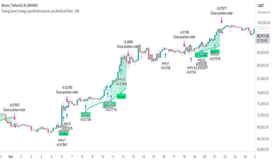
Ultimate Stochastics Strategy by NHBprod Use to Day Trade BTCHey All!
Here's a new script I worked on that's super simple but at the same time useful. Check out the backtest results. The backtest results include slippage and fees/commission, and is still quite profitable. Obviously the profitability magnitude depends on how much capital you begin with, and how much the user utilizes per order, but in any event it seems to be profitable according to backtests.
This is different because it allows you full functionality over the stochastics calculations which is designed for random datasets. This script allows you to:
Designate ANY period of time to analyze and study
Choose between Long trading, short trading, and Long & Short trading
It allows you to enter trades based on the stochastics calculations
It allows you to EXIT trades using the stochastics calculations or take profit, or stop loss, Or any combination of those, which is nice because then the user can see how one variable effects the overall performance.
As for the actual stochastics formula, you get control, and get to SEE the plot lines for slow K, slow D, and fast K, which is usually not considered.
You also get the chance to modify the smoothing method, which has not been done with regular stochastics indicators. You get to choose the standard simple moving average (SMA) method, but I also allow you to choose other MA's such as the HMA and WMA.
Lastly, the user gets the option of using a custom trade extender, which essentially allows a buy or sell signal to exist for X amount of candles after the initial signal. For example, you can use "max bars since signal" to 1, and this will allow the indicator to produce an extra sequential buy signal when a buy signal is generated. This can be useful because it is possible that you use a small take profit (TP) and quickly exit a profitable trade. With the max bars since signal variable, you're able to reenter on the next candle and allow for another opportunity.
Let me know if you have any questions! Please take a look at the performance report and let me know your thoughts! :)
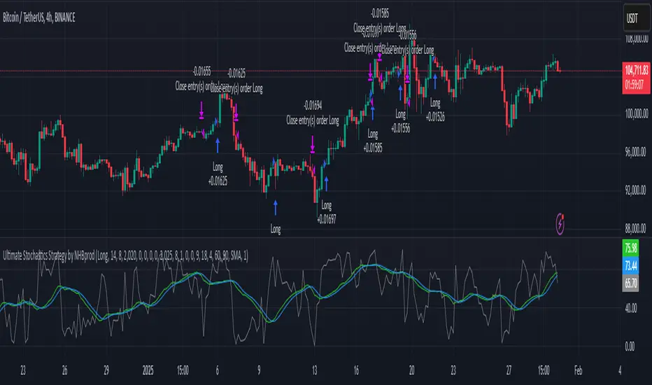
Martingale8MARTINGALE8 Indicator: Comprehensive User Guide
Welcome to the MARTINGALE8 Indicator, your ultimate tool for implementing a customizable martingale trading strategy directly on TradingView! Whether you're a beginner trader or an experienced strategist, this indicator offers flexibility and clarity, empowering you to trade with confidence. Let’s dive into how you can make the most of it!
What Is the Martingale Principle?
The martingale strategy is a betting technique often used in gambling and trading. The idea is simple: double down on losing positions so that when a trade eventually succeeds, the profits will recover all previous losses and yield a small profit. In trading, this translates to placing incrementally larger buy orders as the price moves against your initial position, assuming the price will eventually reverse in your favor.
The martingale principle works under the asumption of mean reversion —that the price will eventually recover to a point where all accumulated losses are recouped, and a profit is made. By increasing order sizes at lower levels, the average entry price moves closer to the current price, reducing the price move required to reach profitability. However, like any strategy, it carries risks — if the price continues to move against your position without reversing, losses can escalate quickly .
What Does MARTINGALE8 Do?
The MARTINGALE8 Indicator is an open source script designed to:
Calculate multiple price levels (buy and take-profit) using a martingale strategy.
Allow full customization of entry size, order deviation, profit targets, and order multipliers.
Visualize key trading levels directly on the chart for better decision-making.
Provide helpful labels with real-time metrics like total cost, range analysis, and high-volume bar prices.
This indicator is ideal for traders looking to automate and refine their martingale-based trading approaches.
Features
1. Customizable Inputs
You have complete control over key parameters:
Start Price: Set a custom starting price, or let it default to the market price.
Entry Size: Choose your initial trade size (default: equivalent to 7.5 USDT).
Order Multiplier: Adjust the size of each subsequent order in the martingale sequence.
Order Deviation: Define the percentage deviation for each buy level.
Profit Deviation: Determine the target percentage deviation for take-profit levels.
Length: Specify the lookback period for market analysis (default: 84 bars).
2. Market Analysis
The script calculates key metrics, including:
Highest Volume Bar (HVB): Identifies the bar with the highest trading volume in the selected period.
Range Analysis: Computes the high-to-low range percentage to help you understand market volatility.
3. Martingale Levels
Automatically generates :
10 Buy Levels: Strategically placed below the starting price.
Take-Profit Level: A target above the starting price based on the profit deviation.
4. Cost Calculation
The script calculates the total cost of all orders, including a 10% buffer for safety, so you can plan your capital allocation effectively.
5. Visual Elements
The indicator draws clean and intuitive lines for:
Take-Profit Level: Highlighted in fuchsia.
Buy Levels: Clearly marked with aqua lines.
Zero Line: Your base price, shown in white.
Additional labels provide:
A summary of key metrics like total cost, entry price, and range.
Precise price values for the take-profit and lowest buy levels.
How to Use MARTINGALE8
Step 1: Add the Indicator to Your Chart
Click on the “Indicators” tab in TradingView.
Search for “MARTINGALE8” and add it to your chart.
Step 2: Configure the Inputs
Navigate to the Settings menu of the indicator and adjust the following parameters:
Start Price : Set your starting price or leave it as 0 to use the current market price.
Entry Size : Define the size of your initial trade (e.g., 7.5 USDT).
Order Multiplier : Choose how much larger each subsequent order should be.
Order Deviation : Specify the percentage distance between buy levels.
Profit Deviation : Set your desired percentage for the take-profit level.
Length : Adjust the number of bars to analyze for high volume.
Step 3: Visualize the Levels
The indicator will plot:
A white line for the base price.
Aqua lines for the buy levels.
A fuchsia line for the take-profit level.
Step 4: Monitor the Labels
Look for the summary label on the chart, which shows:
Total cost of the martingale orders.
Entry price and key market metrics (range, high-volume bar price).
Tips for Optimal Use
Adjust Inputs to Match Market Conditions : Experiment with order and profit deviations to account for volatile or steady markets.
Manage Risk : Use the cost calculation feature to ensure you allocate capital responsibly.
Technical Details
The script is written in Pine Script v6 and uses:
Switch Statements : For flexible default values.
Line Objects : To draw and update key price levels dynamically.
Labels : To display relevant trading metrics.
I’m glad to share this tool with the TradingView community. If you enjoy using MARTINGALE8, please keep it going and share your feedback. Let’s trade smarter, not harder!
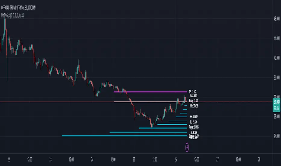
Uptrick: Arbitrage OpportunityINTRODUCTION
This script, titled Uptrick: Arbitrage Monitor, is a Pine Script™ indicator that aims to help traders quickly visualize potential arbitrage scenarios across multiple cryptocurrency exchanges. Arbitrage, in general, involves taking advantage of price differences for the same asset across different trading platforms. By comparing market prices of the same symbol on two user-selected exchanges, as well as scanning a broader list of exchanges, this script attempts to signal areas where you might want to buy on one exchange and sell on another. It includes various graphical tools, calculations, and an optional Automated Detection signal feature, allowing users to incorporate more advanced data scanning into their trading decisions. Keep in mind that transaction fees must also be considered in real-world scenarios. These fees can negate potential profits and, in some cases, result in a net loss.
PURPOSE
The primary purpose of this indicator is to show potential percentage differences between the same cryptocurrency trading pairs on two different exchanges. This difference is displayed numerically, visually as a line chart, and it is also tested against user-defined thresholds. With the threshold in place, buy and sell signals can be generated. The script allows you to quickly gauge how significant a spread is between two exchanges and whether that spread surpasses a specified threshold. This is particularly useful for arbitrage trading, where an asset is bought at a lower price on one exchange and sold at a higher price on another, capitalizing on price discrepancies. By identifying these opportunities, traders can potentially secure profits across different markets.
WHY IT WAS MADE
This script was developed to help traders who frequently look for arbitrage opportunities in the fast-paced cryptocurrency market. Cryptocurrencies sometimes experience quick price divergences across different exchanges. By having an automated approach that compares and displays prices, traders can spend less time manually tracking price discrepancies and more time focusing on actual trading strategies. The script was also made with user customization in mind, allowing you to toggle an optional Automated-based approach and choose different moving average methods to smooth out the displayed price difference.
WHAT ARBITRAGE IS
Arbitrage is the practice of buying an asset on one market (or exchange) at a lower price and simultaneously selling it on another market where the price is higher, thus profiting from the price difference. In cryptocurrency markets, these price differentials can occur across multiple exchanges due to varying liquidity, trading volume, geographic factors, or market inefficiencies. Though sometimes small, these differences can be exploited for profit when approached methodically.
EXPLANATION OF INPUTS
The script includes a variety of user inputs that help tailor the indicator to your specific needs:
1. Compared Symbol 1: This is the primary symbol you want to track (for example, BTCUSDT). Make sure it's written in all capital and make sure that it's price from that exchange is available on Tradingview.
2. Compare Exchange 1: The first exchange on which the script will request pricing data for the chosen symbol.
3. Compared to Exchange: The second exchange, used for the comparison.
4. Opportunity Threshold (%): A percentage threshold that, when exceeded by the price difference, can trigger buy or sell signals.
5. Plot Style?: Allows you to choose between plotting the raw difference line or a moving average of that difference.
6. MA Type: Select among SMA, EMA, WMA, RMA, or HMA for your moving average calculation.
7. MA Length: The lookback period for the selected moving average.
8. Plot Buy/Sell Signals?: Enables or disables the plotting of arrows signaling potential buy or sell zones based on threshold crossovers.
9. Automated Detection?: Toggles an additional multi-exchange data scan feature that calculates the highest and lowest prices for the specified symbol across a predefined list of exchanges.
CALCULATIONS
At its core, the script calculates price1 and price2 using the request.security function to fetch close prices from two selected exchanges. The difference is measured as (price1 - price2) / price2 * 100. This results in a percentage that indicates how much higher or lower price1 is relative to price2. Additionally, the script calculates a slope for this difference, which helps color the line depending on whether it is trending up or down. If you choose the moving average option, the script will replace the raw difference data with one of several moving average calculations (SMA, EMA, WMA, RMA, or HMA).
The script also includes an iterative scan of up to 15 different exchanges for Automated detection, collecting the highest and lowest price across all those exchanges. If the Automated option is enabled, it compiles a potential recommendation: buy at the cheapest exchange price and sell at the most expensive one. The difference across all exchanges (allExDiffPercent) is calculated using (highestPriceAll - lowestPriceAll) / lowestPriceAll * 100.
WHAT AUTOMATED DETECTION SIGNAL DOES
If enabled, the Automated detection feature scans all 15 supported exchanges for the specified symbol. It then identifies the exchange with the highest price and the exchange with the lowest price. The script displays a recommended action: buy on the lowest-exchange price and sell on the highest-exchange price. While called “Automated,” it is essentially a multi-exchange data query that automates a portion of research by consolidating different price points. It does not replace thorough analysis or guaranteed execution; it simply provides an overview of potential extremes.
WHAT ALL-EX-DIFF IS
The variable allExDiffPercent is used to show the overall difference between the highest price and the lowest price found among the 15 pre-chosen exchanges. This figure can be useful for anyone wanting a big-picture view of how large the arbitrage spread might be across the broader market.
SIGNALS AND HOW THEY ARE GENERATED
The script provides two main modes of signal generation:
1. Raw Difference Mode: If the user chooses “Use Normal Line,” the script compares the percentage difference of the two selected exchanges (price1 and price2) to the user-defined threshold. When the difference crosses under the positive threshold, a sell signal is displayed (red arrow). Conversely, when the difference crosses above the negative threshold, a buy signal is displayed (green arrow).
2. Moving Average Mode: If the user selects “Use Moving Average,” the script instead references the moving average values (maValue). The signals fire under similar conditions but use the average line to gauge whether the threshold has been crossed.
HOW TO USE THE INDICATOR
1. Add the script to your chart in TradingView.
2. In the script’s settings panel, configure the symbol you wish to compare (for example, BTCUSDT), choose the two exchanges you want to evaluate, and set your desired threshold.
3. Optionally, pick a moving average type and length if you prefer a smoother representation of the difference.
4. Enable or disable buy/sell signals according to your preference.
5. If you’d like to see potential extremes among a broader list of exchanges, enable Automated Detection. Keep in mind that this feature runs additional security requests, so it might slow down performance on weaker devices or if you already have many scripts running.
EXCHANGES TO USE
The script currently supports up to 15 exchanges: BYBIT, BINANCE, MEXC, BLOFIN, BITGET, OKX, KUCOIN, COINBASE, COINEX, PHEMEX, POLONIEX, GATEIO, BITSTAMP, and KRAKEN. You can choose any two of these for direct comparison, and if you enable the Automated detection, it will attempt to query them all to find extremes in real time.
VISUALS
The exchanges and current prices & differences are all plotted in the table while the colored line represents the difference in the price. The two thresholds colored red are where signals are generated. A cross below the upper threshold is a sell signal and a cross above the lower threshold is a buy signal. In the line at the bottom, purple is a negative slope and aqua is a positive slope.
LIMITATIONS AND POTENTIAL PROBLEMS
If you enable too many visual elements such as signals, additional lines, and the Automated-based scanning table, you may find that your chart becomes cluttered, or text might overlap. One workaround is to remove and reapply the indicator to refresh its display. You may also want to reduce the number of displayed table rows by disabling some features if your chart becomes too crowded. Sometimes there might be an error that the price of an asset is not available on an exchange, to fix this, go and select another exchange to compare it to, or if it happens in Automated detection, choose a different asset, ideally more widely spread.
UNIQUENESS
This indicator stands out due to its multifaceted approach: it doesn’t just look at two exchanges but optionally scans up to 15 exchanges in real time, presenting users with a much broader view of the market. The dual-mode system (raw difference vs. moving average) allows for both immediate, unfiltered signals and smoother, noise-reduced signals depending on user preference. By default, it introduces dynamic visual cues through color changes when the slope of the difference transitions upward or downward. The optional Automated detection, while not a deep learning system, adds a functional intelligence layer by collating extreme price points from multiple exchanges in one place, thereby streamlining the manual research process. This combination of features gives the script a unique edge in the TradingView ecosystem, catering equally to novices wanting a straightforward approach and to advanced users looking for an aggregated multi-exchange analysis.
CONCLUSION
Uptrick: Arbitrage Monitor is a versatile and customizable Pine Script™ indicator that highlights price differences for a specified symbol between two user-selected exchanges. Through signals, threshold-based alerts, and optional Automated detection across multiple exchanges, it aims to support traders in identifying potential arbitrage opportunities quickly and efficiently. This script makes no guarantees of profitability but can serve as a valuable tool to add to your trading toolkit. Always use caution when implementing arbitrage strategies, and be mindful of market risks, exchange fees, and latency.
ADDITIONAL DISCLOSURES
This script is provided for educational and informational purposes only. It does not constitute financial advice or a guarantee of performance. Users are encouraged to conduct thorough research and consider the inherent risks of arbitrage trading. Market conditions can change rapidly, and orders may fail to execute at desired prices, especially when large price discrepancies attract competition from other traders.
TradingIQ - Reversal IQIntroducing "Reversal IQ" by TradingIQ
Reversal IQ is an exclusive trading algorithm developed by TradingIQ, designed to trade trend reversals in the market. By integrating artificial intelligence and IQ Technology, Reversal IQ analyzes historical and real-time price data to construct a dynamic trading system adaptable to various asset and timeframe combinations.
Philosophy of Reversal IQ
Reversal IQ integrates IQ Technology (AI) with the timeless concept of reversal trading. Markets follow trends that inevitably reverse at some point. Rather than relying on rigid settings or manual judgment to capture these reversals, Reversal IQ dynamically designs, creates, and executes reversal-based trading strategies.
Reversal IQ is designed to work straight out of the box. In fact, its simplicity requires just one user setting, making it incredibly straightforward to manage.
AI Aggressiveness is the only setting that controls how Reversal IQ works.
Traders don’t have to spend hours adjusting settings and trying to find what works best - Reversal IQ handles this on its own.
Key Features of Reversal IQ
Self-Learning Reversal Detection
Employs AI and IQ Technology to identify trend reversals in real-time.
AI-Generated Trading Signals
Provides reversal trading signals derived from self-learning algorithms.
Comprehensive Trading System
Offers clear entry and exit labels.
AI-Determined Profit Target and Stop Loss
Position exit levels are clearly defined and calculated by the AI once the trade is entered.
Performance Tracking
Records and presents trading performance data, easily accessible for user analysis.
Configurable AI Aggressiveness
Allows users to adjust the AI's aggressiveness to match their trading style and risk tolerance.
Long and Short Trading Capabilities
Supports both long and short positions to trade various market conditions.
IQ Channel
The IQ Channel represents what Reversal IQ considers a tradable long opportunity or a tradable short opportunity. The channel is dynamic and adjusts from chart to chart.
IQMA – Proprietary Moving Average
Introduces the IQ Moving Average (IQMA), designed to classify overarching market trends.
IQCandles – Trend Classification Tool
Complements IQMA with candlestick colors designed for trend identification and analysis.
How It Works
Reversal IQ operates on a straightforward heuristic: go long during an extended downside move and go short during an extended upside move.
What defines an "extended move" is determined by IQ Technology, TradingIQ's exclusive AI algorithm. For Reversal IQ, the algorithm assesses the extent to which historical high and low prices are breached. By learning from these price level violations, Reversal IQ adapts to trade future, similar violations in a recurring manner. It calculates a price area, distant from the current price, where a reversal is anticipated.
In simple terms, price peaks (tops) and troughs (bottoms) are stored for Reversal IQ to learn from. The degree to which these levels are violated by subsequent price movements is also recorded. Reversal IQ continuously evaluates this stored data, adapting to market volatility and raw price fluctuations to better capture price reversals.
What classifies as a price top or price bottom?
For Reversal IQ, price tops are considered the highest price attained before a significant downside reversal. Price bottoms are considered the lowest price attained before a significant upside reversal. The highest price achieved is continuously calculated before a significant counter trend price move renders the high price as a swing high. The lowest price achieved is continuously calculated before a significant counter trend price move renders the low price as a swing low.
The image above illustrates the IQ channel and explains the corresponding prices and levels
The blue lower line represents the Long Reversal Level, with the price highlighted in blue showing the Long Reversal Price.
The red upper line represents the Short Reversal Level, with the price highlighted in red showing the Short Reversal Price.
Limit orders are placed at both of these levels. As soon as either level is touched, a trade is immediately executed.
The image above shows a long position being entered after the Long Reversal Level was reached. The profit target and stop loss are calculated by Reversal IQ
The blue line indicates where the profit target is placed (acting as a limit order).
The red line shows where the stop loss is placed (acting as a stop loss order).
Green arrows indicate that the strategy entered a long position at the highlighted price level.
You can also hover over the trade labels to get more information about the trade—such as the entry price, profit target, and stop loss.
The image above demonstrates the profit target being hit for the trade. All profitable trades are marked by a blue arrow and blue line. Hover over the blue arrow to obtain more details about the trade exit.
The image above depicts a short position being entered after the Short Reversal Level was touched. The profit target and stop loss are calculated by the AI
The blue line indicates where the profit target is placed (acting as a limit order).
The red line shows where the stop loss is placed (acting as a stop loss order).
The image above shows the profit target being hit for the short trade. Profitable trades are indicated by a blue arrow and blue line. Hover over the blue arrow to access more information about the trade exit.
Long Entry: Green Arrow
Short Entry: Red Arrow
Profitable Trades: Blue Arrow
Losing Trades: Red Arrow
IQMA
The IQMA implements a dynamic moving average that adapts to market conditions by adjusting its smoothing factor based on its own slope. This makes it more responsive in volatile conditions (steeper slopes) and smoother in less volatile conditions.
The IQMA is not used by Reversal IQ as a trade condition; however, the IQMA can be used by traders to characterize the overarching trend and elect to trade only long positions during bullish conditions and only short positions during bearish conditions.
The IQMA is an adaptive smoothing function that applies a combination of multiple moving averages to reduce lag and noise in the data. The adaptiveness is achieved by dynamically adjusting the Volatility Factor (VF) based on the slope (derivative) of the price trend, making it more responsive to strong trends and smoother in consolidating markets.
This process effectively makes the moving average a self-adjusting filter, the IQMA attempts to track both trending and ranging market conditions by dynamically changing its sensitivity in response to price movements.
When IQMA is blue, an overarching uptrend is in place. When IQMA is red, an overarching downtrend is in place.
IQ Candles
IQ Candles are price candles color-coordinated with IQMA. IQ Candles help visualize the overarching trend and are not used by Reversal IQ to determine trade entries and trade exits.
AI Aggressiveness
Reversal IQ has only one setting that controls its functionality.
AI Aggressiveness controls the aggressiveness of the AI. This setting has three options: Sniper, Aggressive, and Very Aggressive.
Sniper Mode
In Sniper Mode, Reversal IQ will prioritize trading large deviations from established reversal levels and extracting the largest countertrend move possible from them.
Aggressive Mode
In Aggressive Mode, Reversal IQ still prioritizes quality but allows for strong, quantity-based signals. More trades will be executed in this mode with tighter stops and profit targets. Aggressive mode forces Reversal IQ to learn from narrower raw-dollar violations of historical levels.
Very Aggressive Mode
In Very Aggressive Mode, Reversal IQ still prioritizes the strongest quantity-based signals. Stop and target distances aren't inherently affected, but entries will be aggressive while prioritizing performance. Very Aggressive mode forces Reversal IQ to learn from narrower raw-dollar violations of historical levels and also forces it to embrace volatility more aggressively.
AI Direction
The AI Direction setting controls the trade direction Reversal IQ is allowed to take.
“Both” allows for both long and short trades.
“Long” allows for only long trades.
“Short” allows for only short trades.
Verifying Reversal IQ’s Effectiveness
Reversal IQ automatically tracks its performance and displays the profit factor for the long strategy and the short strategy it uses. This information can be found in a table located in the top-right corner of your chart.
The image above shows the long strategy profit factor and the short strategy profit factor for Reversal IQ.
A profit factor greater than 1 indicates a strategy profitably traded historical price data.
A profit factor less than 1 indicates a strategy unprofitably traded historical price data.
A profit factor equal to 1 indicates a strategy did not lose or gain money when trading historical price data.
Using Reversal IQ
While Reversal IQ is a full-fledged trading system with entries and exits, it was designed for the manual trader to take its trading signals and analysis indications to greater heights - offering numerous applications beyond its built-in trading system.
The hallmark feature of Reversal IQ is its sniper-like reversal signals. While exits are dynamically calculated as well, Reversal IQ simply has a knack for "sniping" price reversals.
When performing live analysis, you can use the IQ Channel to evaluate price reversal areas, whether price has extended too far in one direction, and whether price is likely to reverse soon.
Of course, in times of exuberance or panic, price may push through the reversal levels. While infrequent, it can happen to any indicator.
The deeper price moves into the bullish reversal area (blue) the better chance that price has extended too far and will reverse to the upside soon. The deeper price moves into the bearish reversal area (red) the better chance that price has extended too far and will reverse to the downside soon.
Of course, you can set alerts for all Reversal IQ entry and exit signals, effectively following along its systematic conquest of price movement.

Fundamental AnalysisThis indicator compiles a wide range of essential financial metrics directly onto your chart, providing a quick and easy reference to the financial condition of any listed company. Instead of diving into lengthy financial reports, you get an at-a-glance overview of the most critical financial ratios and figures.
Key Metrics Included:
Interest Coverage Ratio: Helps assess a company’s ability to pay interest on its debt. Higher values suggest greater financial stability and lower default risk.
Gross Profit Margin: Shows how much profit a company makes after covering its production costs. A higher margin indicates better efficiency and profitability in managing costs.
Dividend Yield: Reflects the annual dividend payout as a percentage of the current stock price. A moderate dividend yield may indicate a balance between income generation and growth potential.
Enterprise Value (EV): A comprehensive measure of a company's total value, including debt. Useful for comparing companies with different capital structures.
Free Cash Flow to Equity (FCFE): Reveals how much cash is available to shareholders after accounting for capital expenditures and debt repayments, indicating the company’s ability to reward investors.
Price-to-Book Ratio (P/B): Compares a company's market value to its book value. Lower values might indicate undervaluation, while higher values can suggest overvaluation.
Price-to-Cash Flow Ratio (P/CF): Helps identify companies that generate a significant amount of cash relative to their price, a key metric for assessing liquidity and sustainability.
Price-to-Free Cash Flow Ratio: Shows how much investors are paying for the company's free cash flow, which is crucial for assessing value, especially in capital-intensive sectors.
Price Earnings Ratio (P/E): The classic metric for valuing a company based on its earnings. Useful for comparing valuations across companies and industries.
Debt-to-Equity Ratio: Indicates the proportion of company financing that comes from debt and equity. A lower ratio typically signifies a less risky investment.
Return on Equity (ROE): Measures how effectively a company uses equity capital to generate profit. A higher ROE can indicate a profitable, well-managed company.
Quick Ratio: Assesses a company’s short-term liquidity by comparing its liquid assets to its current liabilities. Higher values indicate better liquidity.
Operating Margin: Reflects the percentage of revenue left after covering operating expenses. Higher margins suggest greater operational efficiency.
How to Use This Indicator:
Use this indicator as part of your due diligence when analyzing potential investments. Each metric is color-coded to quickly highlight whether the value is within a favorable range, making it easy to identify strong or weak aspects of a company’s financial position.
Green indicates favorable metrics, suggesting financial strength or value.
Red highlights areas of concern, pointing to potential risks or weaknesses.
This tool can help you compare different companies, spot trends over time, and make more informed decisions based on solid financial analysis. Whether you’re a value investor looking for undervalued stocks, a dividend seeker searching for sustainable payouts, or a growth investor focused on profitability and efficiency, this indicator can be tailored to your strategy.

Nifty scalping 3 minutesOverview:
The "Nifty Scalping 3 Minutes" strategy is a uniquely tailored trading system for Nifty Futures traders, with a clear focus on capital preservation, dynamic risk management, and high-probability trade entries. This strategy uses unique combination of standard technical indicators like Jurik Moving Average (JMA), Exponential Moving Average (EMA), and Bollinger Bands, but it truly stands out through its Price-Volume Spike Detection system—a unique mechanism designed to trigger trades only during periods of high momentum and market participation. The strategy also incorporates robust risk management, ensuring that traders minimize losses while maximizing profits. in complete back test range max drawdown is less than 1%
Scalping Approach and Requirements:
The strategy focuses on quick in and out trades, aiming to capture small, quick profits during periods of heightened market activity. For optimal performance, traders should have ₹2,00,000 or more in capital available per trade. The dynamic lot calculation and risk controls require this level of capital to function effectively.
Small, frequent trades are the focus, and the strategy is ideal for traders comfortable with high-frequency executions. Traders with insufficient capital or those not comfortable with frequent trades may find this strategy unsuitable.
Default Properties for Publication:
Initial Capital: ₹2,000,000
Lot Size: 25 contracts (adjusted dynamically based on available margin)
Stop-Loss: Risk per trade capped at 1% of equity.
Slippage and Commission: Realistic values are factored into the backtesting.
Key Feature: Price-Volume Spike Detection
1. Condition: Trades are executed only when there is a significant price spike confirmed by a volume spike. The candle width is calculated by multiplying the price change (difference between the candle's open and close) by the volume, and this result is compared to a 126-period average of both price and volume.
A trade is triggered when the current price-volume spike exceeds this average by a preset volume multiplier (default set at 3). This ensures that both the price change and volume are unusually strong compared to normal market behavior.
2. Reasoning: Many traders fail to incorporate the relationship between price movement and volume effectively. By using this Price-Volume Spike Detection mechanism, the strategy ensures that it only enters trades during periods of strong market momentum when both price and volume confirm a real market move, not just noise or small fluctuations.
The 126-period moving average of volume is chosen specifically because it represents a complete trading session on the 3-minute chart. This ensures that the volume spike is compared against a realistic baseline of daily activity, making the detection more robust and reliable.
The volume multiplier allows flexibility in determining the threshold for a significant spike, enabling users to fine-tune the strategy according to their risk tolerance and market conditions.
Trade Placement Logic:
1. Trend Confirmation with JMA and EMA:
Condition: The strategy will only consider entering a trade when JMA crosses above EMA for a long trade or JMA crosses below EMA for a short trade.
Reasoning: The JMA is used for its low lag and responsiveness, allowing it to capture early trends, while the EMA adds a level of confirmation by weighing recent price action more heavily. This dual confirmation ensures that trades are entered only when a solid trend is in place.
2. Bollinger Bands for Volatility Breakouts:
Condition: In addition to the JMA-EMA crossover, the price must break outside the Bollinger Bands—above the upper band for long trades, or below the lower band for short trades.
Reasoning: Bollinger Bands are a volatility indicator. By requiring a price breakout beyond the bands, the strategy ensures that trades are placed during periods of high volatility, avoiding low-momentum, sideways markets.
3. Volume and Price Confirmation (Price-Volume Spike Detection):
Condition: A trade is only triggered if the price-volume spike condition is met. This ensures that the market move is backed by strong volume and that the price change is significant relative to the recent average activity.
Reasoning: This condition filters out low-volume environments where price movements are more likely to reverse or stall. By waiting for a spike in both price and volume, the strategy ensures that it enters trades during high-momentum periods, where follow-through is more likely.
Exit Logic and Risk Management:
1. Stop-Loss (SL) Placement:
Condition: Upon entering a trade, an initial stop-loss is placed below the candle low for long trades or above the candle high for short trades. This is adjusted if the risk exceeds 1% of total capital.
Reasoning: The stop-loss is placed at a logical level that accounts for recent price action, ensuring that the trade is given room to develop while protecting capital from unexpected market reversals.
2. Profit Target and Partial Profit Booking:
Condition: The first profit target is set at 2.1x the initial risk for long trades, and 2.5x the initial risk for short trades.
Reasoning: The 2.1x risk-reward ratio for long trades provides a solid return while maintaining a conservative risk profile. For short trades, the strategy uses a higher 2.5x risk-reward ratio because market falls tend to be sharper and quicker than rises, allowing for larger profit targets to be reached more reliably.
Partial Profit Booking: Once the first target is hit, 60% of the position is closed to lock in profits. The remaining 40% is left to run with a trailing stop.
3. ATR-Based Trailing Stop:
Condition: Once the first target is hit, the ATR (Average True Range) trailing stop is applied to the remaining position. This dynamically adjusts the stop-loss as the trade moves in a favorable direction.
Reasoning: The trailing stop allows the trade to capture further gains if the trend continues, while protecting profits if the momentum weakens. The ATR ensures that the stop adjusts according to the market's current volatility, providing flexibility and protection.
4. Time-Based Exit:
Condition: If a trade is still open by 3:20 PM, it is automatically closed to avoid end-of-day volatility.
Reasoning: The time-based exit ensures that trades are not held into the often-volatile closing minutes of the market, reducing the risk of unexpected price swings.
Capital and Risk Management:
1. Lot Size Calculation:
Condition: The strategy calculates the number of lots dynamically based on the available margin. It uses only 10% of total equity for each trade, and ensures that the maximum risk per trade does not exceed 1% of total capital.
Reasoning: This ensures that traders are not over-leveraged and that the risk is controlled for each trade. Capital protection is at the core of the strategy, ensuring that even during adverse market conditions, the trader’s capital is preserved.
2. Stop-Loss Protection:
Condition: The stop-loss is designed to ensure that no more than 1% of capital is at risk in any trade.
Reasoning: By limiting risk exposure, the strategy focuses on long-term capital preservation while still allowing for profitable trades in favorable market conditions.
STBT/BTST Facilitation:
1. Feature: The strategy allows traders the option to hold positions overnight, facilitating STBT (Sell Today Buy Tomorrow) and BTST (Buy Today Sell Tomorrow) trades.
Reasoning: Backtests show that holding positions overnight when all trade conditions are still valid can lead to beneficial outcomes. This feature allows traders to take advantage of overnight market movements, providing flexibility beyond intraday trades.
Why This Strategy Stands Out:
Price-Volume Spike Detection: Unlike traditional strategies, this one uniquely focuses on Price-Volume Spike Detection to filter out low-probability trades. By ensuring that both price and volume spikes are present, the strategy guarantees that trades are placed only when there is significant market momentum.
Risk Management with Capital Protection: The strategy strictly limits the risk per trade to 1% of capital, ensuring long-term capital preservation. This is especially important for traders who wish to avoid large drawdowns and prefer a sustainable approach to trading.
2.5x Risk-Reward for Short Trades: Recognizing the sharpness of market declines, the strategy employs a 2.5x risk-reward ratio for short trades, maximizing profits during bearish trends.
Dynamic Exit Strategy: With partial profit booking and ATR-based trailing stops, the strategy is designed to capture gains efficiently while protecting capital through dynamic exit conditions.
Summary of Execution:
Entry: Triggered when JMA crosses EMA, combined with Bollinger Band breakouts and Price-Volume Spike Detection.
Capital Management: Trades are executed with 10% of available capital, and the risk per trade is capped at 1%.
Exit: Trades exit when stop-loss, ATR trailing stop, or time-based exit conditions are met.
Profit Booking: 60% of the position is closed at the first target, with the remainder trailed using an ATR-based stop.

Dow Theory based Strategy (Markttechnik)What makes this script unique?
calculates two trends at the same time: a big one for the overall strong trend - and a small one to trigger a trade after a small correction within the big trend
only if both trends (the small and the big trend) are in an uptrend, a buy signal is created: this prevents a buy signal from being generated in a falling market just because an upward movement begins in a small trend
the exit strategy can be configured very flexibly and individually: use the last low as stop loss and automatically switch to a trialing stop loss as soon as the take profit is reached (instead of finishing the trade)
the take profit strategy can also be configured - e.g. use the last high, a fixed percentage or a combination of it
plots each trade in detail on the chart - e.g. inner candles or the exact progression of the stop loss over the entire duration of the trade to allow you to analyze each trade precisely
What does the script do and how?
In this strategy an intact upward trend is characterized by higher highs and lower lows only if the big trend and the small trend are in an upward trend at the same time.
The following describes how the script calculates a buy signal. Every step is drawn to the chart immediately - see example chart above:
1. the stock rises in the big trend - i.e. in a longer time frame
2. a correction takes place (the share price falls) - but does not create a new low
3. the stock rises again in the big trend and creates a new high
From now on, the big trend is in an intact upward trend (until it falls below its last low).
This is drawn to the chart as 3 bold green zigzag lines.
But we do not buy right now! Instead, we want to wait for a correction in the big trend and for the start of a small upward trend.
4. a correction takes place (not below the low from 2.)
Now, the script also starts to calculate the small trend:
5. the stock rises in the small trend - i.e. in a shorter time frame
6. a small correction takes place (not below the low from 4.)
7. the stock rises above the high from 5.: a new high in the shorter time frame
Now, both trends are in an intact upward trend.
A buy signal is created and both the minor and major trend are colored green on the chart.
Now, the trade is active and:
the stop loss is calculated and drawn for each candle
the take profit is calculated and drawn to the chart
as soon as the price reaches the take profit or the stop loss, the trade is closed
Features and functionalities
Uptrend : An intact upward trend is characterized by higher highs and lower lows. Uptrends are shown in green on the chart.
The beginning of an uptrend is numbered 1, each subsequent high is numbered 2, and each low is numbered 3.
Downtrend: An intact downtrend is characterized by lower highs and lower lows. Downtrends are displayed in red on the chart.
Note that our indicator does not show the numbering of the points of the downtrend.
Trendless phases: If there is no intact trend, we are in a trendless phase. Trendless phases are shown in blue on the chart.
This occurs after an uptrend, when a lower low or a lower high is formed. Or after a downtrend, when a higher low or a higher high is formed.
Buy signals
A buy signal is generated as soon as a new upward trend has been formed or a new high has been established in an intact upward trend.
But even before a buy signal is generated, this strategy anticipates a possible emerging trend and draws the next possible trading opportunity to the chart.
In addition to the (not yet reached) buy price, the risk-reward ratio, the StopLoss and the TakeProfit price is shown.
With this information, you can already enter a StopBuy order, which is thus triggered directly with the then created buy signal.
You can configure, if a buy signal shall be created while the big trend is an uptrend, a downtrend and/or trendless.
Exit strategy
With this strategy, you have multiple possibilities to close your position. All of them can be configured within the settings. In general, you can combine a take profit strategy with a stop loss strategy.
The take profit price will be calculated once for each trade. It will be drawn to the chart for active trade.
Depending on your configuration, this can be the last high (which is often a resistance level), a fixed percentage added to the buy price or the maximum of both.
You can also configure that a trailing stop loss is used as soon as the take profit price is reached once.
The stop loss gets recalculated with each candle and is displayed and plotted for each active and finished trade. With this, you can easily check how the stop loss changed during your trades.
The stop loss can be configured flexibly:
Use the classic "trailing stop loss" that follows the price from below.
Set the stop loss to the last low and tighten it every time the small trend marks a new local low.
Confiure that the stop loss is tightened as soon as the break even is reached. Nothing is more annoying than a trade turning from a win to a loss.
Ignore inside candles (see description below) and relax the stop loss to use the outside candle for its calculation.
Inner candles
Inner candles are created when the candle body is within the maximum values of a previous candle (the outer candle). There can be any number of consecutive inner candles. As soon as you have activated the "Check inner candles" setting, all consecutive inner candles will be highlighted in yellow on the chart.
Prices during an inner candle scenario might be irrelevant for trading and can be interpreted as fluctuations within the outside candle. For this reason, the trailing stop loss should not be aligned with inner candles. Therefore, as soon as an inner candle occurs, the stop loss is reset and the low at the time of the outside candle is used as the calculation for the trailing stop loss. This will all be plotted for you on the chart.
Display of the trades:
All active and closed trades of the last 5 years are displayed in the chart with buy signal, sell, stop loss history, inside candles and statistics.
Backtesting:
The strategy can be simulated for each stock over the period of the last 5 years. Each individual trade is recorded and can be traced and analyzed in the chart including stop loss history. Detailed evaluations and statistics are available to evaluate the performance of the strategy.
Additional Statistics
This strategy immediately displays a statistic table to the chart area giving you an overview of its performance over the last years for the given chart.
This includes:
The total win/loss in $ and %
The win/loss per year in %
The active investment time in days and % (e.g. invested 10 of 100 trading days -> 10%)
The total win/loss in %, extrapolated to 100% equity usage: Only with this value can strategies really be compared. Because you are not invested between the trades and could invest in other stocks during this time. This value indicates how much profit you would have made if you had been invested 100% of the time - or to put it another way - if you had been invested 100% of the time in stocks with exactly the same performance. Let's say you had only one trade in the last 5 years that lasted, say, only one month and made 5% profit. This would be significantly better than a strategy with which you were invested for, say, 5 years and made 10% profit.
The total profit/loss per year in %, extrapolated to 100% equity usage
Notifications (alerts):
Get alerted before a new buy signal emerges to create an order if necessary and not miss a trade. You can also be notified when the stop loss needs to be adjusted. The notification can be done in different ways, e.g. by Mail, PopUp or App-Notification. This saves them the annoying, time-consuming and error-prone "click through" all the charts.
Settings: Display Settings
With these settings, you have the possibility to:
Show the small or the big trend as a background color
Configure if the numbers (1-2-3-2-3) shall be shown at all or only for the small, the big trend or both
Settings: Trend calculation - fine tuning
Drawing trend lines on a chart is not an exact science. Some highs and lows are not very clear or significant. And so it will always happen that 2 different people would draw different trendlines for the same chart. Unfortunately, there is no exact "right" or "wrong" here.
With the options under "Trend Calculation - Fine Tuning" you have the possibility to influence the drawing in of trends and to adapt it to your personal taste.
Small Trend, Big Trend : With these settings you can influence how significant a high or low has to be to recognize them as an independent high or low. The larger the values, the more significant a high or low must be to be recognized as such.
High and low recognition : With this setting you can influence when two adjacent, almost identical highs or lows should be recognized as independent highs or lows. The higher the value, the more different "similar" highs or lows must be in order to be recognized as such.
Which default settings were selected and why
Show Trades: true - its often useful to see all recent trades in the chart
Time Frame: 1 day - most common time frame (except for day traders)
Take Profit: combined 10% - the last high is taken as take profit because the trend often changes there, but only if there is at least 10% profit to ensure we do not risk money for a tiny profit
Stop Loss: combined - the last low is used as stop loss because the trend would break there and switch to a trailing stop loss as soon as our take profit is reached to let our profits run without risking them anymore
Stop Loss distance: 3% - we are giving the price 3% air (below the last low) to avoid being stopped out due to a short price drop
Trailing Stop Loss: 2% - we have to give the stop loss some room to avoid being stopped out prematurely; this is a value that is well balanced between a certain downside distance and the profit-taking ratio
Set Stop Loss to break even: true, 2% - once we reached the break even, it is a common practice to not risk our money anymore, the value is set to the same value as the trailing stop loss
Trade Filter: Uptrend - we only start trades if the big trend is an uptrend in the expectation that it will continue after a small correction
Display settings: those will not influence the trades, feel free to change them to your needs
Trend calculation - Fine Tuning: 1/1,5/0,05; influences the internal calculation for highs and lows and how significant they need to be to be considered a new high or low; the default values will provide you nicely calculated trends in the daily time frame; if there are too many or too few lows and highs according to your taste, feel free to play around and immediately see the result drawn to the chart; read the manual for a detailed description of this values
Note that you can (and should) configure the general trading properties like your initial capital, order size, slippage and commission.

Uptrick: RSI Histogram
1. **Introduction to the RSI and Moving Averages**
2. **Detailed Breakdown of the Uptrick: RSI Histogram**
3. **Calculation and Formula**
4. **Visual Representation**
5. **Customization and User Settings**
6. **Trading Strategies and Applications**
7. **Risk Management**
8. **Case Studies and Examples**
9. **Comparison with Other Indicators**
10. **Advanced Usage and Tips**
---
## 1. Introduction to the RSI and Moving Averages
### **1.1 Relative Strength Index (RSI)**
The Relative Strength Index (RSI) is a momentum oscillator developed by J. Welles Wilder and introduced in his 1978 book "New Concepts in Technical Trading Systems." It is widely used in technical analysis to measure the speed and change of price movements.
**Purpose of RSI:**
- **Identify Overbought/Oversold Conditions:** RSI values range from 0 to 100. Traditionally, values above 70 are considered overbought, while values below 30 are considered oversold. These thresholds help traders identify potential reversal points in the market.
- **Trend Strength Measurement:** RSI also indicates the strength of a trend. High RSI values suggest strong bullish momentum, while low values indicate bearish momentum.
**Calculation of RSI:**
1. **Calculate the Average Gain and Loss:** Over a specified period (e.g., 14 days), calculate the average gain and loss.
2. **Compute the Relative Strength (RS):** RS is the ratio of average gain to average loss.
3. **RSI Formula:** RSI = 100 - (100 / (1 + RS))
### **1.2 Moving Averages (MA)**
Moving Averages are used to smooth out price data and identify trends by filtering out short-term fluctuations. Two common types are:
**Simple Moving Average (SMA):** The average of prices over a specified number of periods.
**Exponential Moving Average (EMA):** A type of moving average that gives more weight to recent prices, making it more responsive to recent price changes.
**Smoothed Moving Average (SMA):** Used to reduce the impact of volatility and provide a clearer view of the underlying trend. The RMA, or Running Moving Average, used in the USH script is similar to an EMA but based on the average of RSI values.
## 2. Detailed Breakdown of the Uptrick: RSI Histogram
### **2.1 Indicator Overview**
The Uptrick: RSI Histogram (USH) is a technical analysis tool that combines the RSI with a moving average to create a histogram that reflects momentum and trend strength.
**Key Components:**
- **RSI Calculation:** Determines the relative strength of price movements.
- **Moving Average Application:** Smooths the RSI values to provide a clearer trend indication.
- **Histogram Plotting:** Visualizes the deviation of the smoothed RSI from a neutral level.
### **2.2 Indicator Purpose**
The primary purpose of the USH is to provide a clear visual representation of the market's momentum and trend strength. It helps traders identify:
- **Bullish and Bearish Trends:** By showing how far the smoothed RSI is from the neutral 50 level.
- **Potential Reversal Points:** By highlighting changes in momentum.
### **2.3 Indicator Design**
**RSI Moving Average (RSI MA):** The RSI MA is a smoothed version of the RSI, calculated using a running moving average. This smooths out short-term fluctuations and provides a clearer indication of the underlying trend.
**Histogram Calculation:**
- **Neutral Level:** The histogram is plotted relative to the neutral level of 50. This level represents a balanced market where neither bulls nor bears have dominance.
- **Histogram Values:** The histogram bars show the difference between the RSI MA and the neutral level. Positive values indicate bullish momentum, while negative values indicate bearish momentum.
## 3. Calculation and Formula
### **3.1 RSI Calculation**
The RSI calculation involves:
1. **Average Gain and Loss:** Calculated over the specified length (e.g., 14 periods).
2. **Relative Strength (RS):** RS = Average Gain / Average Loss.
3. **RSI Formula:** RSI = 100 - (100 / (1 + RS)).
### **3.2 Moving Average Calculation**
For the USH indicator, the RSI is smoothed using a running moving average (RMA). The RMA formula is similar to that of the EMA but is based on averaging RSI values over the specified length.
### **3.3 Histogram Calculation**
The histogram value is calculated as:
- **Histogram Value = RSI MA - 50**
**Plotting the Histogram:**
- **Positive Histogram Values:** Indicate that the RSI MA is above the neutral level, suggesting bullish momentum.
- **Negative Histogram Values:** Indicate that the RSI MA is below the neutral level, suggesting bearish momentum.
## 4. Visual Representation
### **4.1 Histogram Bars**
The histogram is plotted as bars on the chart:
- **Bullish Bars:** Colored green when the RSI MA is above 50.
- **Bearish Bars:** Colored red when the RSI MA is below 50.
### **4.2 Customization Options**
Traders can customize:
- **RSI Length:** Adjust the length of the RSI calculation to match their trading style.
- **Bull and Bear Colors:** Choose colors for histogram bars to enhance visual clarity.
### **4.3 Interpretation**
**Bullish Signal:** A histogram bar that moves from red to green indicates a potential shift to a bullish trend.
**Bearish Signal:** A histogram bar that moves from green to red indicates a potential shift to a bearish trend.
## 5. Customization and User Settings
### **5.1 Adjusting RSI Length**
The length parameter determines the number of periods over which the RSI is calculated and smoothed. Shorter lengths make the RSI more sensitive to price changes, while longer lengths provide a smoother view of trends.
### **5.2 Color Settings**
Traders can adjust:
- **Bull Color:** Color of histogram bars indicating bullish momentum.
- **Bear Color:** Color of histogram bars indicating bearish momentum.
**Customization Benefits:**
- **Visual Clarity:** Traders can choose colors that stand out against their chart’s background.
- **Personal Preference:** Adjust settings to match individual trading styles and preferences.
## 6. Trading Strategies and Applications
### **6.1 Trend Following**
**Identifying Entry Points:**
- **Bullish Entry:** When the histogram changes from red to green, it signals a potential entry point for long positions.
- **Bearish Entry:** When the histogram changes from green to red, it signals a potential entry point for short positions.
**Trend Confirmation:** The histogram helps confirm the strength of a trend. Strong, consistent green bars indicate robust bullish momentum, while strong, consistent red bars indicate robust bearish momentum.
### **6.2 Swing Trading**
**Momentum Analysis:**
- **Entry Signals:** Look for significant shifts in the histogram to time entries. A shift from bearish to bullish (red to green) indicates potential for upward movement.
- **Exit Signals:** A shift from bullish to bearish (green to red) suggests a potential weakening of the trend, signaling an exit or reversal point.
### **6.3 Range Trading**
**Market Conditions:**
- **Consolidation:** The histogram close to zero suggests a range-bound market. Traders can use this information to identify support and resistance levels.
- **Breakout Potential:** A significant move away from the neutral level may indicate a potential breakout from the range.
### **6.4 Risk Management**
**Stop-Loss Placement:**
- **Bullish Positions:** Place stop-loss orders below recent support levels when the histogram is green.
- **Bearish Positions:** Place stop-loss orders above recent resistance levels when the histogram is red.
**Position Sizing:** Adjust position sizes based on the strength of the histogram signals. Strong trends (indicated by larger histogram bars) may warrant larger positions, while weaker signals suggest smaller positions.
## 7. Risk Management
### **7.1 Importance of Risk Management**
Effective risk management is crucial for long-term trading success. It involves protecting capital, managing losses, and optimizing trade setups.
### **7.2 Using USH for Risk Management**
**Stop-Loss and Take-Profit Levels:**
- **Stop-Loss Orders:** Use the histogram to set stop-loss levels based on trend strength. For instance, place stops below support levels in bullish trends and above resistance levels in bearish trends.
- **Take-Profit Targets:** Adjust take-profit levels based on histogram changes. For example, lock in profits as the histogram starts to shift from green to red.
**Position Sizing:**
- **Trend Strength:** Scale position sizes based on the strength of histogram signals. Larger histogram bars indicate stronger trends, which may justify larger positions.
- **Volatility:** Consider market volatility and adjust position sizes to mitigate risk.
## 8. Case Studies and Examples
### **8.1 Example 1: Bullish Trend**
**Scenario:** A trader notices a transition from red to green histogram bars.
**Analysis:**
- **Entry Point:** The transition indicates a potential bullish trend. The trader decides to enter a long position.
- **Stop-Loss:** Set stop-loss below recent support levels.
- **Take-Profit:** Consider taking profits as the histogram moves back towards zero or turns red.
**Outcome:** The bullish trend continues, and the histogram remains green, providing a profitable trade setup.
### **8.2 Example 2: Bearish Trend**
**Scenario:** A trader observes a transition from green to red histogram bars.
**Analysis:**
- **Entry Point:** The transition suggests a potential
bearish trend. The trader decides to enter a short position.
- **Stop-Loss:** Set stop-loss above recent resistance levels.
- **Take-Profit:** Consider taking profits as the histogram approaches zero or shifts to green.
**Outcome:** The bearish trend continues, and the histogram remains red, resulting in a successful trade.
## 9. Comparison with Other Indicators
### **9.1 RSI vs. USH**
**RSI:** Measures momentum and identifies overbought/oversold conditions.
**USH:** Builds on RSI by incorporating a moving average and histogram to provide a clearer view of trend strength and momentum.
### **9.2 RSI vs. MACD**
**MACD (Moving Average Convergence Divergence):** A trend-following momentum indicator that uses moving averages to identify changes in trend direction.
**Comparison:**
- **USH:** Provides a smoothed RSI perspective and visual histogram for trend strength.
- **MACD:** Offers signals based on the convergence and divergence of moving averages.
### **9.3 RSI vs. Stochastic Oscillator**
**Stochastic Oscillator:** Measures the level of the closing price relative to the high-low range over a specified period.
**Comparison:**
- **USH:** Focuses on smoothed RSI values and histogram representation.
- **Stochastic Oscillator:** Provides overbought/oversold signals and potential reversals based on price levels.
## 10. Advanced Usage and Tips
### **10.1 Combining Indicators**
**Multi-Indicator Strategies:** Combine the USH with other technical indicators (e.g., Moving Averages, Bollinger Bands) for a comprehensive trading strategy.
**Confirmation Signals:** Use the USH to confirm signals from other indicators. For instance, a bullish histogram combined with a moving average crossover may provide a stronger buy signal.
### **10.2 Customization Tips**
**Adjust RSI Length:** Experiment with different RSI lengths to match various market conditions and trading styles.
**Color Preferences:** Choose histogram colors that enhance visibility and align with personal preferences.
### **10.3 Continuous Learning**
**Backtesting:** Regularly backtest the USH with historical data to refine strategies and improve accuracy.
**Education:** Stay updated with trading education and adapt strategies based on market changes and personal experiences.

CPR By Ask Dinesh Kumar(ADK)Simple CPR Indicator to increase probability of profitable trades:
The Central Pivot Range (CPR) is a trading tool used by traders to identify potential support and resistance levels in the market. Here's a simplified explanation of how traders can potentially profit using the Central Pivot Range with 10 lines:
1. *Understanding CPR*: CPR consists of three lines: the pivot point (PP), upper resistance level (R1), and lower support level (S1). Additionally, traders often add five more of profitable tradeslines above and below the PP to create a 10-line CPR.
2. *Identify Trend*: Determine the prevailing market trend. If the market is bullish, traders will look for buying opportunities near support levels. If the market is bearish, they'll seek selling opportunities near resistance levels.
3. *Entry Points*: Look for entry points near the support (S1) or resistance (R1) levels within the CPR. These levels can act as potential turning points where price may reverse.
4. *Risk Management*: Set stop-loss orders to manage risk. Stop-loss orders should be placed slightly below support levels for long positions and slightly above resistance levels for short positions.
5. *Profit Targets*: Determine profit targets based on the distance between entry point and the next support or resistance level. Some traders use a risk-reward ratio to ensure potential profits outweigh potential losses.
6. *Confirmation*: Use additional technical indicators or price action patterns to confirm potential entry or exit points within the CPR.
7. *Monitor Price Action*: Continuously monitor price action around the CPR levels. Traders should be prepared to adjust their positions if price breaks through support or resistance levels convincingly.
8. *Trade Management*: Once in a trade, actively manage it by adjusting stop-loss orders, trailing stops, or taking partial profits as price moves in the desired direction.
9. *Market Conditions*: Consider broader market conditions, such as economic indicators, geopolitical events, or news releases, which can impact price movements and the effectiveness of CPR.
10. *Practice and Analysis*: Practice using CPR on historical price charts and analyze past trades to refine strategies and improve decision-making skills.
Remember, trading involves risks, and no strategy guarantees profits. It's essential to thoroughly understand the concepts behind CPR and practice disciplined risk management to increase the likelihood of successful trades.
How does central pivot range work:
Sure here's a concise explanation of how the Central Pivot Range (CPR) works in 10 points:
1. *Calculation*: CPR is calculated using the previous day's high (H), low (L), and close (C) prices.
2. *Pivot Point (PP)*: The central point of CPR is the average of the previous day's high, low, and close prices: PP = (H + L + C) / 3.
3. *Upper Resistance Levels (R1, R2, R3)*: These are potential price levels above the pivot point where resistance may occur. They are calculated by adding a multiple of the range (H - L) to the pivot point: R1 = (2 * PP) - L, R2 = PP + (H - L), R3 = PP + 2 * (H - L).
4. *Lower Support Levels (S1, S2, S3)*: These are potential price levels below the pivot point where support may occur. They are calculated similarly to resistance levels but subtracting multiples of the range from the pivot point: S1 = (2 * PP) - H, S2 = PP - (H - L), S3 = PP - 2 * (H - L).
5. *Trading Signals*: Traders use CPR to identify potential support and resistance levels where price may reverse or stall.
6. *Range Bound Markets*: In range-bound markets, traders may buy near support levels (S1, S2, S3) and sell near resistance levels (R1, R2, R3).
7. *Breakout Trading*: When price breaks through a CPR level convincingly, it may indicate a potential trend continuation or reversal, providing breakout trading opportunities.
8. *Volume and Momentum*: Traders often look for confirmation from volume and momentum indicators when price approaches CPR levels.
9. *Intraday Trading*: CPR can be applied to intraday timeframes as well, providing shorter-term traders with potential trading levels for the day.
10. *Dynamic Indicator*: CPR is dynamic and recalculates daily based on new price data, allowing traders to adapt their strategies to current market conditions.
Understanding how to interpret CPR levels and integrate them into a trading strategy can help traders identify potential entry and exit points in the market.
Strategic Multi-Step Supertrend - Strategy [presentTrading]The code is mainly developed for me to stimulate the multi-step taking profit function for strategies. The result shows the drawdown can be reduced but at the same time reduced the profit as well. It can be a heuristic for futures leverage traders.
█ Introduction and How it is Different
The "Strategic Multi-Step Supertrend" is a trading strategy designed to leverage the power of multiple steps to optimize trade entries and exits across the Supertrend indicator. Unlike traditional strategies that rely on single entry and exit points, this strategy employs a multi-step approach to take profit, allowing traders to lock in gains incrementally. Additionally, the strategy is adaptable to both long and short trades, providing a comprehensive solution for dynamic market conditions.
This template strategy lies in its dual Supertrend calculation, which enhances the accuracy of trend detection and provides more reliable signals for trade entries and exits. This approach minimizes false signals and increases the overall profitability of trades by ensuring that positions are entered and exited at optimal points.
BTC 6h L/S Performance
█ Strategy, How It Works: Detailed Explanation
The "Strategic Multi-Step Supertrend Trader" strategy utilizes two Supertrend indicators calculated with different parameters to determine the direction and strength of the market trend. This dual approach increases the robustness of the signals, reducing the likelihood of entering trades based on false signals. Here is a detailed breakdown of how the strategy operates:
🔶 Supertrend Indicator Calculation
The Supertrend indicator is a trend-following overlay on the price chart, typically used to identify the direction of the trend. It is calculated using the Average True Range (ATR) to ensure that the indicator adapts to market volatility. The formula for the Supertrend indicator is:
Upper Band = (High + Low) / 2 + (Factor * ATR)
Lower Band = (High + Low) / 2 - (Factor * ATR)
Where:
- High and Low are the highest and lowest prices of the period.
- Factor is a user-defined multiplier.
- ATR is the Average True Range over a specified period.
The Supertrend changes its direction based on the closing price in relation to these bands.
🔶 Entry-Exit Conditions
The strategy enters long positions when both Supertrend indicators signal an uptrend, and short positions when both indicate a downtrend. Specifically:
- Long Condition: Supertrend1 < 0 and Supertrend2 < 0
- Short Condition: Supertrend1 > 0 and Supertrend2 > 0
- Long Exit Condition: Supertrend1 > 0 and Supertrend2 > 0
- Short Exit Condition: Supertrend1 < 0 and Supertrend2 < 0
🔶 Multi-Step Take Profit Mechanism
The strategy features a multi-step take profit mechanism, which allows traders to lock in profits incrementally. This is achieved through four user-configurable take profit levels. For each level, the strategy specifies a percentage increase (for long trades) or decrease (for short trades) in the entry price at which a portion of the position is exited:
- Step 1: Exit a portion of the trade at Entry Price * (1 + Take Profit Percent1 / 100)
- Step 2: Exit a portion of the trade at Entry Price * (1 + Take Profit Percent2 / 100)
- Step 3: Exit a portion of the trade at Entry Price * (1 + Take Profit Percent3 / 100)
- Step 4: Exit a portion of the trade at Entry Price * (1 + Take Profit Percent4 / 100)
This staggered exit strategy helps in locking profits at multiple levels, thereby reducing risk and increasing the likelihood of capturing the maximum possible profit from a trend.
BTC Local
█ Trade Direction
The strategy is highly flexible, allowing users to specify the trade direction. There are three options available:
- Long Only: The strategy will only enter long trades.
- Short Only: The strategy will only enter short trades.
- Both: The strategy will enter both long and short trades based on the Supertrend signals.
This flexibility allows traders to adapt the strategy to various market conditions and their own trading preferences.
█ Usage
1. Add the strategy to your trading platform and apply it to the desired chart.
2. Configure the take profit settings under the "Take Profit Settings" group.
3. Set the trade direction under the "Trade Direction" group.
4. Adjust the Supertrend settings in the "Supertrend Settings" group to fine-tune the indicator calculations.
5. Monitor the chart for entry and exit signals as indicated by the strategy.
█ Default Settings
- Use Take Profit: True
- Take Profit Percentages: Step 1 - 6%, Step 2 - 12%, Step 3 - 18%, Step 4 - 50%
- Take Profit Amounts: Step 1 - 12%, Step 2 - 8%, Step 3 - 4%, Step 4 - 0%
- Number of Take Profit Steps: 3
- Trade Direction: Both
- Supertrend Settings: ATR Length 1 - 10, Factor 1 - 3.0, ATR Length 2 - 11, Factor 2 - 4.0
These settings provide a balanced starting point, which can be customized further based on individual trading preferences and market conditions.
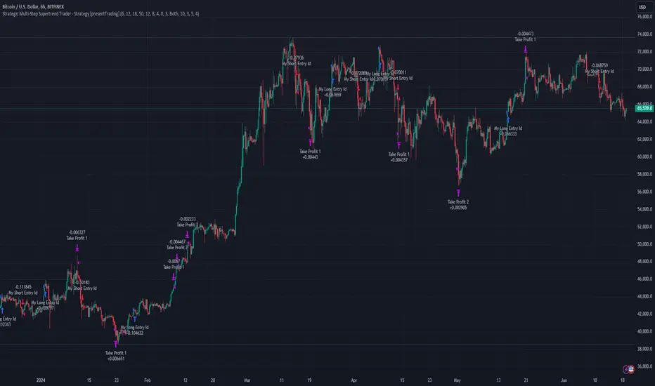
Buffett Quality Score [Financials]Evaluating Financial Companies with the Buffett Quality Score 'Financials'
The financial sector, with its unique regulatory environment and market dynamics, requires a tailored approach to financial evaluation. The Buffett Quality Score is meticulously designed to assess the financial robustness and quality of companies within this sector. By focusing on industry-specific financial metrics, this scoring system provides valuable insights for investors and analysts navigating the complexities of the financial industry.
Scoring Methodology
Each selected financial metric contributes a point to the overall score if the specified condition is met. The combined score is a summation of points across all criteria, providing a comprehensive assessment of financial health and quality.
Selected Financial Metrics and Criteria
1. Altman Z-Score > 2.0
Relevance: The Altman Z-Score evaluates bankruptcy risk based on profitability, leverage, liquidity, solvency, and activity. In the financial sector, where market stability and solvency are critical, a score above 2.0 signifies a lower risk of financial distress.
2. Debt to Equity Ratio < 2.0
Relevance: A lower Debt to Equity Ratio signifies prudent financial management and reduced reliance on debt financing. This is particularly important for financial companies, which need to manage leverage carefully to avoid excessive risk.
3. Interest Coverage > 3.0
Relevance: The Interest Coverage Ratio measures a company's ability to meet its interest obligations from operating earnings. A ratio above 3.0 indicates that the company can comfortably cover its interest expenses, reducing the risk of default.
4. Return on Equity (ROE) > 10.0%
Relevance: ROE indicates the company's ability to generate profits from shareholder equity. An ROE above 10.0% suggests efficient use of capital and strong returns for investors, which is a key performance indicator for financial companies.
5. Return on Assets (ROA) > 1.0%
Relevance: ROA measures the company's ability to generate earnings from its assets. In the financial sector, where asset management is crucial, an ROA above 1.0% indicates effective use of assets to generate profits.
6. Net Margin > 10.0%
Relevance: Net Margin measures overall profitability after all expenses. A margin above 10.0% demonstrates strong financial performance and the ability to convert revenue into profit effectively.
7. Revenue One-Year Growth > 5.0%
Relevance: Revenue growth reflects market demand and company expansion. In the financial sector, where growth can be driven by new products and services, revenue exceeding 5.0% indicates successful market penetration and business expansion.
8. EPS One-Year Growth > 5.0%
Relevance: EPS growth reflects the company's ability to increase earnings per share over the past year. For financial companies, growth exceeding 5.0% signals positive earnings momentum and potential market strength.
9. Price/Earnings Ratio (Forward) < 20.0
Relevance: The Forward P/E Ratio reflects investor sentiment and earnings expectations. A ratio below 20.0 suggests reasonable valuation relative to earnings projections, which is important for investors seeking value and growth opportunities in the financial sector.
10. Piotroski F-Score > 6.0
Relevance: The Piotroski F-Score assesses fundamental strength, emphasizing profitability, leverage, liquidity, and operating efficiency. For financial companies, a score above 6.0 indicates strong financial health and operational efficiency.
Interpreting the Buffett Quality Score
0-4 Points: Indicates potential weaknesses across multiple financial areas, warranting careful consideration and risk assessment.
5 Points: Suggests average performance based on sector-specific criteria, requiring further analysis to determine investment viability.
6-10 Points: Signifies strong financial health and quality, positioning the company favorably within the competitive financial industry.
Conclusion
The Buffett Quality Score offers a strategic framework for evaluating financial companies, emphasizing critical financial indicators tailored to industry dynamics. By leveraging these insights, stakeholders can make informed decisions and identify companies poised for sustainable growth and performance in the evolving financial landscape.
Disclaimer: The Buffett Quality Score serves as a tool for financial analysis and should not replace professional advice or comprehensive due diligence. Investors should conduct thorough research and consult with financial experts based on individual investment objectives.
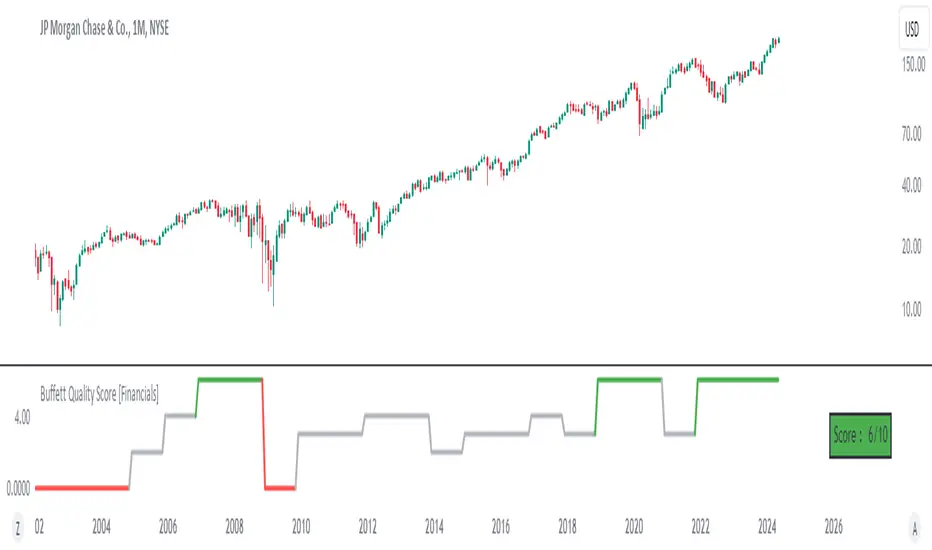
Pullback_Power [JackTz]Welcome to Pullback_Power
Pullback_Power is a scalping strategy designed to capitalize on market retracements while incorporating unique dynamic features to enhance profitability.
Calculation
Pullback_Power purely uses moving averages to calculate both entry and exits. Exits can also be set to fixed percentages for both take profit and stop loss.
How the Strategy Works
Statistics show that markets normally do a recovery after each drop. Crypto markets can easily drop up to 20% within a few hours and then do a complete or partial recovery. Pullback_Power utilizes this known pattern alongside pyramiding. The strategy aims to catch one or more entries when the price drops, hoping to make profits when the market recovers from the drop. The fixed take profit and stop loss can be used to define your risk management, while the dynamic exit opportunity is riskier but provides the ability to stay in the trade longer while it recovers. Pullback_Power can make up to four entries. This means it utilizes pyramiding to spread out the entry points, but every exit is a full exit. It is not possible to partially exit.
Utility
Pullback_Power is a scalping strategy suitable for traders who operate with small trades and don't want to stay in the market for too long. Pullback_Power offers precise signals with no repainting. The strategy thrives in volatility, so crypto pairs might yield the best results, although this strategy can be adapted to work on all pairs and markets.
How to Automate It
Pullback_Power utilizes the standard placeholders of strategies on TradingView. This enables the trader to add every data point into a webhook, making it fully flexible to suit every trader's needs. To automate, create an alert, set the webhook URL, and add the JSON body needed for the webhook. An example of a simple JSON webhook with some of the standard strategy placeholders:
{
"side": "{{strategy.order.action}}",
"symbol": "{{ticker}}",
"amount": "{{strategy.order.contracts}}"
}
Read about all the standard placeholders that you can use here: TradingView - Standard strategy placeholders
Originality
Pullback_Power is unique in its ability to create precise signals without repainting while maintaining a solid approach to the pullback strategy. Its simplicity not only makes the strategy easy to use and understand but also highly effective. The simplicity reduces inputs, eliminating overfitting and limits each input to avoid incorrect usage. Many times, default settings are enough to achieve good backtesting results on almost all pairs available. Pullback_Power also differs from many other strategies by its solid code, which enhances performance and provides more reliable backtesting. The clean code increases the resilience and precision of the entries, making it less prone to errors.
Many pullback/scalping strategies normally only works on specific scopes of timeframes or pairs. Pullback_Power can easily be adapted to work on almost every scenario. The biggest change needed is the length of the moving average. The lower the timeframe, the higher a length is needed for proper results. I.e. on a 2H timeframe a length of 3 can yield good results. On a 5min timeframe the length might need to be as high as 70.
How to Use
To use Pullback_Power, add the script to your trading chart. By default, Pullback_Power opens four orders to optimize trade opportunities with a default fee value set at 0.1%. You can change these default settings in the Settings window under the Properties tab. To tailor Pullback_Power to your individual trading style, navigate to the Settings under the Input tab. Here you can configure various inputs to fit your trading style.
- Backtest settings , Start Date:
Defines the date of when the calculation starts. Use this to set the date of when the first trade could potentially emit.
- Backtest settings , End Date:
Defines the date of when the calculation ends. If there are any open trades after this date the close calculations are still live. It only makes sure that new orders cannot be opened after this date.
- Backtest settings , Only trade on weekdays:
This is a toggle you can enable or disable. If enabled it only allows new entries to happen during the normal week days, meaning Monday, Tuesday, Wednesday, Thursday and Friday.
Disable this to enable the script to open trades on all 7 days of the week.
- Open settings , Use dynamic long positions:
This toggle allows you to enable or disable the pullback level calculations after first trade.
If enabled, the calculations of level 2, 3 and 4 continues to happen after each bar, making the levels follow the price with the moving averages calculations.
If disabled, the calculations of the levels stop after the first trade. This means that the levels calculation at the point of the first trade stay fixed until all trades are closed.
You can see the difference of the green lines on the chart when you toggle this flag.
- Open settings , Data type:
This is the bar data used for the moving average calculation when opening trades. The possible data types are Open, High, Low, Close, HL2, HLC3, OHLC4, OC2 and HC2.
- Open settings , Source type:
This is the source used to calculate the moving average. The types available are: SMA, PCMA, EMA, WMA, DEMA, ZLEMA and HMA.
- Open settings , Length:
This is the length used for the moving average calculations. 3 means it takes the last 3 bars of historical data for the calculation.
- Open settings , Offset:
This defines if the calculation should use an offset for the historical data. This does not use a look-forward feature, but a look-backward feature. To prevent any possible repaints the offset can only be positive, not negative.
For instance, if the length is 3 and the offset is 0 the calculation is made from the last 3 bars, making it bar1, bar2 and bar3. If the length is 3 and the offset is 1 the calculation is made from bar2, bar3, and bar4 – offsetting the calculation by 1 bar.
- Leverage settings , Leverage liquidation (1-125):
The script itself does not handle any custom leverage calculation – this must be done in the Properties tabs and increasing the order size.
This setting is made to test a possible liquidation event if using leverage.
By setting this to higher than 1, a red line is visible after the first trade on the chart. This indicates the liquidation price.
If this setting is set to 25, the script will calculate the liquidation price from a x25 leverage. If this price is hit, the scripts stops emitting any orders and the background turns red.
You can use this to test if your settings could handle a certain level of leverage.
- Pullback settings , Pullback 1, 2, 3 and 4:
Each of these settings defines the entry price of each pullback level. If Pullback 1 is set to -6 it means that the moving average calculation should be 6% lower than the actual price.
The same logic applies to Pullback 2, 3 and 4.
Setting any level to 0 will disable the level – eliminating any orders to emit on that level.
This can be used to change the level of pyramiding down from 4 if needed.
If you do this, remember to also change the order size and the pyramiding value in the Properties tab accordingly.
- Close settings , Use dynamic TP and SL:
If enabled, script will exit all orders using the same but separate algorithm for moving averages. This enables the user to define if you want the orders to be closed if the price level of this moving average is hit. The price level for this calculation is visible on the chart by the blue line.
Although you can change the length and offset, as described underneath, this calculation uses the same data and source type defined in the Open settings area.
- Close settings , Length, Close:
This is the length used for the closing moving average calculations. 3 means it takes the last 3 bars of historical data for the calculation.
- Close settings , Offset, Close:
This defines if the calculation for the closing moving average should use an offset for the historical data. Just as the offset used for opening order, this does not use a look-forward feature, but a look-backward feature. To prevent any possible repaints the offset can only be positive, not negative.
For instance, if the length is 3 and the offset is 0 the calculation is made from the last 3 bars, making it bar1, bar2 and bar3. If the length is 3 and the offset is 1 the calculation is made from bar2, bar3, and bar4 – offsetting the calculation by 1 bar.
- Close settings , Use TakeProfit:
This toggle enables/disables a fixed take profit percentage.
- Close settings , TP %:
This sets the wanted % to reach on a take profit. This setting is ignored if the toggle above is disabled.
- Close settings , Use StopLoss:
This toggle enables/disables a fixed stop loss percentage.
- Close settings , SL %:
This sets the wanted % to reach on a stop loss. This setting is ignored if the toggle above is disabled.
Exit on Same Bar as Entry
By default, the script doesn't emit any exit orders on the same bar as the first entry order. Enable "Recalculation: After order is filled" to change this behavior.
Troubleshooting
While Pullback_Power is designed to provide reliable trading signals, you may encounter rare issues. One such issue could be receiving an error message stating "can't open orders with 0 or negative qty." If you encounter this error, it is likely due to specific conditions on the selected timeframe. To resolve this issue, change the timeframe on your trading chart.
Underlying Principles and Value Proposition
Pullback_Power leverages moving averages and volatility behavior to identify market retracements and capitalize on them. The strategy is rooted in the understanding that markets often experience temporary reversals or "pullbacks" before resuming their primary trend. By identifying these pullbacks and entering trades at opportune moments, Pullback_Power aims to capture quick profits from short-term market movements.
The dynamic and fixed calculations of Take Profit (TP) and Stop Loss (SL) levels enhances risk management, ensuring that potential losses are controlled while allowing room for profits to grow. The adaptive approach using the moving averages considers current market conditions, making the strategy flexible and responsive to changing volatility.
Moreover, Pullback_Power's non-repainting nature ensures the reliability of its signals, eliminating hindsight bias and providing traders with actionable insights based on real-time market data.
The strategy's simplicity and effectiveness make it accessible for traders of all experience levels. Whether you're a beginner looking to start scalping or an experienced trader seeking to diversify your trading approach, Pullback_Power offers a balanced blend of simplicity and sophistication to help you navigate the markets with confidence.
By focusing on clear, transparent principles and offering practical tools for risk management, Pullback_Power aims to provide tangible value to traders, empowering them to make informed decisions and optimize their trading outcomes.
Thank you for choosing Pullback_Power. I wish you successful trading!
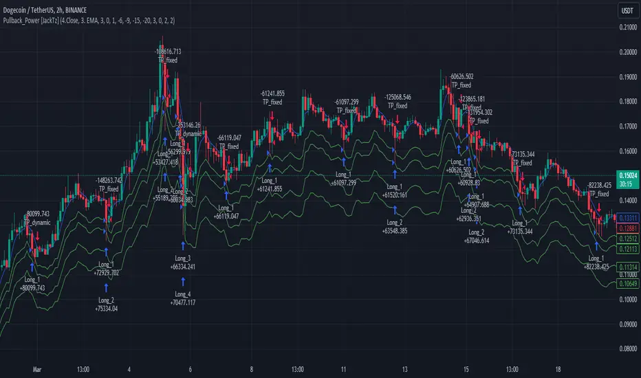
Candlestick Patterns detection and backtester [TrendX_]INTRODUCTION:
The Candlestick Patterns detection and backtester is designed to empower traders by identifying and analyzing candlestick patterns. Leveraging the robust Pine Script's add-in “All Candlestick Patterns”, this indicator meticulously scans the market for candlestick formations, offering insights into potential market movements. With its backtesting capabilities, we evaluate historical data to present traders with performance metrics such as win rates, net profit, and profit factors for each pattern. This allows traders to make informed decisions based on empirical evidence. The customizable settings, including trend filters and exit conditions, provide a tailored experience, adapting to various trading styles and strategies.
CREDIT:
This indicator is powered by the Pinescript add-in, *All Candlestick Patterns*, which provides a comprehensive library of candlestick formations.
TABLE USAGE:
The indicator features a detailed usage table that presents backtested results of all candlestick patterns. This includes:
Win Rates: The percentage of trades that resulted in a profit.
Net Profit: The total profit after subtracting losses from gains.
Profit Factor: A measure of the indicator’s profitability (gross profit / gross loss).
Total Trades: The total number of trades taken for every candlestick pattern's appearance.
CHART CANDLESTICK USAGE:
The indicator integrates candlestick pattern detections directly into the chart, displaying:
Pattern Detections: Each detected pattern is marked on the chart.
Win Rates: The win rate of each pattern is shown in brackets next to the detection.
CHART SETTINGS:
Users can customize the indicator with a variety of trend filters and settings:
Trend Filters: Apply filters based on SMA50, SMA200, Supertrend, and RSI threshold to refine pattern detections.
Exit Condition: Set an exit condition based on the crossing of a simple moving average of customizable length.
Visibility: Choose to show or hide the candlestick patterns’ detections on the chart.

GKD-B Multi-Ticker Stepped Baseline [Loxx]Giga Kaleidoscope GKD-B Multi-Ticker Stepped Baseline is a Baseline module included in Loxx's "Giga Kaleidoscope Modularized Trading System".
This version of the GKD-B Baseline is designed specifically to support traders who wish to conduct GKD-BT Multi-Ticker Backtests with multiple tickers. This functionality is exclusive to the GKD-BT Multi-Ticker Backtests.
Traders have the capability to apply a filter to the selected moving average, leveraging various volatility metrics to enhance trend identification. This feature is tailored for traders favoring a gradual and consistent approach, enabling them to discern more sustainable trends. The system permits filtering for both the input data and the moving average results, requiring price movements to exceed a specific threshold—defined as multiples of the volatility—before acknowledging a trend change. This mechanism effectively reduces false signals caused by market noise and lateral movements. A distinctive aspect of this tool is its ability to adjust both price and moving average data based on volatility indicators like VIX, EUVIX, BVIV, and EVIV, among others. Understanding the time frame over which a volatility index is measured is crucial; for instance, VIX is measured on an annual basis, whereas BVIV and EVIV are based on a 30-day period. To accurately convert these measurements to a daily scale, users must input the correct "days per year" value: 252 for VIX and 30 for BVIV and EVIV. Future updates will introduce additional functionality to extend analysis across various time frames, but currently, this feature is solely available for daily time frame analysis.
█ GKD-B Multi-Ticker Stepped Baseline includes 65+ different moving averages:
Adaptive Moving Average - AMA
ADXvma - Average Directional Volatility Moving Average
Ahrens Moving Average
Alexander Moving Average - ALXMA
Deviation Scaled Moving Average - DSMA
Donchian
Double Exponential Moving Average - DEMA
Double Smoothed Exponential Moving Average - DSEMA
Double Smoothed FEMA - DSFEMA
Double Smoothed Range Weighted EMA - DSRWEMA
Double Smoothed Wilders EMA - DSWEMA
Double Weighted Moving Average - DWMA
Ehlers Optimal Tracking Filter - EOTF
Exponential Moving Average - EMA
Fast Exponential Moving Average - FEMA
Fractal Adaptive Moving Average - FRAMA
Generalized DEMA - GDEMA
Generalized Double DEMA - GDDEMA
Hull Moving Average (Type 1) - HMA1
Hull Moving Average (Type 2) - HMA2
Hull Moving Average (Type 3) - HMA3
Hull Moving Average (Type 4) - HMA4
IE /2 - Early T3 by Tim Tilson
Integral of Linear Regression Slope - ILRS
Kaufman Adaptive Moving Average - KAMA
Laguerre Filter
Leader Exponential Moving Average
Linear Regression Value - LSMA ( Least Squares Moving Average )
Linear Weighted Moving Average - LWMA
McGinley Dynamic
McNicholl EMA
Non-Lag Moving Average
Ocean NMA Moving Average - ONMAMA
One More Moving Average - OMA
Parabolic Weighted Moving Average
Probability Density Function Moving Average - PDFMA
Quadratic Regression Moving Average - QRMA
Regularized EMA - REMA
Range Weighted EMA - RWEMA
Recursive Moving Trendline
Simple Decycler - SDEC
Simple Jurik Moving Average - SJMA
Simple Moving Average - SMA
Sine Weighted Moving Average
Smoothed LWMA - SLWMA
Smoothed Moving Average - SMMA
Smoother
Super Smoother
T3
Three-pole Ehlers Butterworth
Three-pole Ehlers Smoother
Triangular Moving Average - TMA
Triple Exponential Moving Average - TEMA
Two-pole Ehlers Butterworth
Two-pole Ehlers smoother
Variable Index Dynamic Average - VIDYA
Variable Moving Average - VMA
Volume Weighted EMA - VEMA
Volume Weighted Moving Average - VWMA
Zero-Lag DEMA - Zero Lag Exponential Moving Average
Zero-Lag Moving Average
Zero Lag TEMA - Zero Lag Triple Exponential Moving Average
Geometric Mean Moving Average
Coral
Tether Lines
Range Filter
Triangle Moving Average Generalized
Ultinate Smoother
Adaptive Moving Average - AMA
The Adaptive Moving Average (AMA) is a moving average that changes its sensitivity to price moves depending on the calculated volatility. It becomes more sensitive during periods when the price is moving smoothly in a certain direction and becomes less sensitive when the price is volatile.
ADXvma - Average Directional Volatility Moving Average
Linnsoft's ADXvma formula is a volatility-based moving average, with the volatility being determined by the value of the ADX indicator.
The ADXvma has the SMA in Chande's CMO replaced with an EMA , it then uses a few more layers of EMA smoothing before the "Volatility Index" is calculated.
A side effect is, those additional layers slow down the ADXvma when you compare it to Chande's Variable Index Dynamic Average VIDYA .
The ADXVMA provides support during uptrends and resistance during downtrends and will stay flat for longer, but will create some of the most accurate market signals when it decides to move.
Ahrens Moving Average
Richard D. Ahrens's Moving Average promises "Smoother Data" that isn't influenced by the occasional price spike. It works by using the Open and the Close in his formula so that the only time the Ahrens Moving Average will change is when the candlestick is either making new highs or new lows.
Alexander Moving Average - ALXMA
This Moving Average uses an elaborate smoothing formula and utilizes a 7 period Moving Average. It corresponds to fitting a second-order polynomial to seven consecutive observations. This moving average is rarely used in trading but is interesting as this Moving Average has been applied to diffusion indexes that tend to be very volatile.
Deviation Scaled Moving Average - DSMA
The Deviation-Scaled Moving Average is a data smoothing technique that acts like an exponential moving average with a dynamic smoothing coefficient. The smoothing coefficient is automatically updated based on the magnitude of price changes. In the Deviation-Scaled Moving Average, the standard deviation from the mean is chosen to be the measure of this magnitude. The resulting indicator provides substantial smoothing of the data even when price changes are small while quickly adapting to these changes.
Donchian
Donchian Channels are three lines generated by moving average calculations that comprise an indicator formed by upper and lower bands around a midrange or median band. The upper band marks the highest price of a security over N periods while the lower band marks the lowest price of a security over N periods.
Double Exponential Moving Average - DEMA
The Double Exponential Moving Average ( DEMA ) combines a smoothed EMA and a single EMA to provide a low-lag indicator. It's primary purpose is to reduce the amount of "lagging entry" opportunities, and like all Moving Averages, the DEMA confirms uptrends whenever price crosses on top of it and closes above it, and confirms downtrends when the price crosses under it and closes below it - but with significantly less lag.
Double Smoothed Exponential Moving Average - DSEMA
The Double Smoothed Exponential Moving Average is a lot less laggy compared to a traditional EMA . It's also considered a leading indicator compared to the EMA , and is best utilized whenever smoothness and speed of reaction to market changes are required.
Double Smoothed FEMA - DSFEMA
Same as the Double Exponential Moving Average (DEMA), but uses a faster version of EMA for its calculation.
Double Smoothed Range Weighted EMA - DSRWEMA
Range weighted exponential moving average (EMA) is, unlike the "regular" range weighted average calculated in a different way. Even though the basis - the range weighting - is the same, the way how it is calculated is completely different. By definition this type of EMA is calculated as a ratio of EMA of price*weight / EMA of weight. And the results are very different and the two should be considered as completely different types of averages. The higher than EMA to price changes responsiveness when the ranges increase remains in this EMA too and in those cases this EMA is clearly leading the "regular" EMA. This version includes double smoothing.
Double Smoothed Wilders EMA - DSWEMA
Welles Wilder was frequently using one "special" case of EMA (Exponential Moving Average) that is due to that fact (that he used it) sometimes called Wilder's EMA. This version is adding double smoothing to Wilder's EMA in order to make it "faster" (it is more responsive to market prices than the original) and is still keeping very smooth values.
Double Weighted Moving Average - DWMA
Double weighted moving average is an LWMA (Linear Weighted Moving Average). Instead of doing one cycle for calculating the LWMA, the indicator is made to cycle the loop 2 times. That produces a smoother values than the original LWMA
Ehlers Optimal Tracking Filter - EOTF
The Elher's Optimum Tracking Filter quickly adjusts rapid shifts in the price and yet is relatively smooth when the price has a sideways action. The operation of this filter is similar to Kaufman’s Adaptive Moving
Average
Exponential Moving Average - EMA
The EMA places more significance on recent data points and moves closer to price than the SMA ( Simple Moving Average ). It reacts faster to volatility due to its emphasis on recent data and is known for its ability to give greater weight to recent and more relevant data. The EMA is therefore seen as an enhancement over the SMA .
Fast Exponential Moving Average - FEMA
An Exponential Moving Average with a short look-back period.
Fractal Adaptive Moving Average - FRAMA
The Fractal Adaptive Moving Average by John Ehlers is an intelligent adaptive Moving Average which takes the importance of price changes into account and follows price closely enough to display significant moves whilst remaining flat if price ranges. The FRAMA does this by dynamically adjusting the look-back period based on the market's fractal geometry.
Generalized DEMA - GDEMA
The double exponential moving average (DEMA), was developed by Patrick Mulloy in an attempt to reduce the amount of lag time found in traditional moving averages. It was first introduced in the February 1994 issue of the magazine Technical Analysis of Stocks & Commodities in Mulloy's article "Smoothing Data with Faster Moving Averages.". Instead of using fixed multiplication factor in the final DEMA formula, the generalized version allows you to change it. By varying the "volume factor" form 0 to 1 you apply different multiplications and thus producing DEMA with different "speed" - the higher the volume factor is the "faster" the DEMA will be (but also the slope of it will be less smooth). The volume factor is limited in the calculation to 1 since any volume factor that is larger than 1 is increasing the overshooting to the extent that some volume factors usage makes the indicator unusable.
Generalized Double DEMA - GDDEMA
The double exponential moving average (DEMA), was developed by Patrick Mulloy in an attempt to reduce the amount of lag time found in traditional moving averages. It was first introduced in the February 1994 issue of the magazine Technical Analysis of Stocks & Commodities in Mulloy's article "Smoothing Data with Faster Moving Averages''. This is an extension of the Generalized DEMA using Tim Tillsons (the inventor of T3) idea, and is using GDEMA of GDEMA for calculation (which is the "middle step" of T3 calculation). Since there are no versions showing that middle step, this version covers that too. The result is smoother than Generalized DEMA, but is less smooth than T3 - one has to do some experimenting in order to find the optimal way to use it, but in any case, since it is "faster" than the T3 (Tim Tillson T3) and still smooth, it looks like a good compromise between speed and smoothness.
Hull Moving Average (Type 1) - HMA1
Alan Hull's HMA makes use of weighted moving averages to prioritize recent values and greatly reduce lag whilst maintaining the smoothness of a traditional Moving Average. For this reason, it's seen as a well-suited Moving Average for identifying entry points. This version uses SMA for smoothing.
Hull Moving Average (Type 2) - HMA2
Alan Hull's HMA makes use of weighted moving averages to prioritize recent values and greatly reduce lag whilst maintaining the smoothness of a traditional Moving Average. For this reason, it's seen as a well-suited Moving Average for identifying entry points. This version uses EMA for smoothing.
Hull Moving Average (Type 3) - HMA3
Alan Hull's HMA makes use of weighted moving averages to prioritize recent values and greatly reduce lag whilst maintaining the smoothness of a traditional Moving Average. For this reason, it's seen as a well-suited Moving Average for identifying entry points. This version uses LWMA for smoothing.
Hull Moving Average (Type 4) - HMA4
Alan Hull's HMA makes use of weighted moving averages to prioritize recent values and greatly reduce lag whilst maintaining the smoothness of a traditional Moving Average. For this reason, it's seen as a well-suited Moving Average for identifying entry points. This version uses SMMA for smoothing.
IE /2 - Early T3 by Tim Tilson and T3 new
The T3 moving average is a type of technical indicator used in financial analysis to identify trends in price movements. It is similar to the Exponential Moving Average (EMA) and the Double Exponential Moving Average (DEMA), but uses a different smoothing algorithm.
The T3 moving average is calculated using a series of exponential moving averages that are designed to filter out noise and smooth the data. The resulting smoothed data is then weighted with a non-linear function to produce a final output that is more responsive to changes in trend direction.
The T3 moving average can be customized by adjusting the length of the moving average, as well as the weighting function used to smooth the data. It is commonly used in conjunction with other technical indicators as part of a larger trading strategy.
Integral of Linear Regression Slope - ILRS
A Moving Average where the slope of a linear regression line is simply integrated as it is fitted in a moving window of length N (natural numbers in maths) across the data. The derivative of ILRS is the linear regression slope. ILRS is not the same as a SMA ( Simple Moving Average ) of length N, which is actually the midpoint of the linear regression line as it moves across the data.
Kaufman Adaptive Moving Average - KAMA
Developed by Perry Kaufman, Kaufman's Adaptive Moving Average (KAMA) is a moving average designed to account for market noise or volatility. KAMA will closely follow prices when the price swings are relatively small and the noise is low.
Laguerre Filter
The Laguerre Filter is a smoothing filter which is based on Laguerre polynomials. The filter requires the current price, three prior prices, a user defined factor called Alpha to fill its calculation.
Adjusting the Alpha coefficient is used to increase or decrease its lag and its smoothness.
Leader Exponential Moving Average
The Leader EMA was created by Giorgos E. Siligardos who created a Moving Average which was able to eliminate lag altogether whilst maintaining some smoothness. It was first described during his research paper "MACD Leader" where he applied this to the MACD to improve its signals and remove its lagging issue. This filter uses his leading MACD's "modified EMA" and can be used as a zero lag filter.
Linear Regression Value - LSMA ( Least Squares Moving Average )
LSMA as a Moving Average is based on plotting the end point of the linear regression line. It compares the current value to the prior value and a determination is made of a possible trend, eg. the linear regression line is pointing up or down.
Linear Weighted Moving Average - LWMA
LWMA reacts to price quicker than the SMA and EMA . Although it's similar to the Simple Moving Average , the difference is that a weight coefficient is multiplied to the price which means the most recent price has the highest weighting, and each prior price has progressively less weight. The weights drop in a linear fashion.
McGinley Dynamic
John McGinley created this Moving Average to track prices better than traditional Moving Averages. It does this by incorporating an automatic adjustment factor into its formula, which speeds (or slows) the indicator in trending, or ranging, markets.
McNicholl EMA
Dennis McNicholl developed this Moving Average to use as his center line for his "Better Bollinger Bands" indicator and was successful because it responded better to volatility changes over the standard SMA and managed to avoid common whipsaws.
Non-lag moving average
The Non Lag Moving average follows price closely and gives very quick signals as well as early signals of price change. As a standalone Moving Average, it should not be used on its own, but as an additional confluence tool for early signals.
Ocean NMA Moving Average - ONMAMA
Created by Jim Sloman, the NMA is a moving average that automatically adjusts to volatility without being programmed to do so. For more info, read his guide "Ocean Theory, an Introduction"
One More Moving Average (OMA)
The One More Moving Average (OMA) is a technical indicator that calculates a series of Jurik-style moving averages in order to reduce noise and provide smoother price data. It uses six exponential moving averages to generate the final value, with the length of the moving averages determined by an adaptive algorithm that adjusts to the current market conditions. The algorithm calculates the average period by comparing the signal to noise ratio and using this value to determine the length of the moving averages. The resulting values are used to generate the final value of the OMA, which can be used to identify trends and potential changes in trend direction.
Parabolic Weighted Moving Average
The Parabolic Weighted Moving Average is a variation of the Linear Weighted Moving Average . The Linear Weighted Moving Average calculates the average by assigning different weights to each element in its calculation. The Parabolic Weighted Moving Average is a variation that allows weights to be changed to form a parabolic curve. It is done simply by using the Power parameter of this indicator.
Probability Density Function Moving Average - PDFMA
Probability density function based MA is a sort of weighted moving average that uses probability density function to calculate the weights. By its nature it is similar to a lot of digital filters.
Quadratic Regression Moving Average - QRMA
A quadratic regression is the process of finding the equation of the parabola that best fits a set of data. This moving average is an obscure concept that was posted to Forex forums in around 2008.
Regularized EMA - REMA
The regularized exponential moving average (REMA) by Chris Satchwell is a variation on the EMA (see Exponential Moving Average) designed to be smoother but not introduce too much extra lag.
Range Weighted EMA - RWEMA
This indicator is a variation of the range weighted EMA. The variation comes from a possible need to make that indicator a bit less "noisy" when it comes to slope changes. The method used for calculating this variation is the method described by Lee Leibfarth in his article "Trading With An Adaptive Price Zone".
Recursive Moving Trendline
Dennis Meyers's Recursive Moving Trendline uses a recursive (repeated application of a rule) polynomial fit, a technique that uses a small number of past values estimations of price and today's price to predict tomorrow's price.
Simple Decycler - SDEC
The Ehlers Simple Decycler study is a virtually zero-lag technical indicator proposed by John F. Ehlers. The original idea behind this study (and several others created by John F. Ehlers) is that market data can be considered a continuum of cycle periods with different cycle amplitudes. Thus, trending periods can be considered segments of longer cycles, or, in other words, low-frequency segments. Applying the right filter might help identify these segments.
Simple Loxx Moving Average - SLMA
A three stage moving average combining an adaptive EMA, a Kalman Filter, and a Kauffman adaptive filter.
Simple Moving Average - SMA
The SMA calculates the average of a range of prices by adding recent prices and then dividing that figure by the number of time periods in the calculation average. It is the most basic Moving Average which is seen as a reliable tool for starting off with Moving Average studies. As reliable as it may be, the basic moving average will work better when it's enhanced into an EMA .
Sine Weighted Moving Average
The Sine Weighted Moving Average assigns the most weight at the middle of the data set. It does this by weighting from the first half of a Sine Wave Cycle and the most weighting is given to the data in the middle of that data set. The Sine WMA closely resembles the TMA (Triangular Moving Average).
Smoothed LWMA - SLWMA
A smoothed version of the LWMA
Smoothed Moving Average - SMMA
The Smoothed Moving Average is similar to the Simple Moving Average ( SMA ), but aims to reduce noise rather than reduce lag. SMMA takes all prices into account and uses a long lookback period. Due to this, it's seen as an accurate yet laggy Moving Average.
Smoother
The Smoother filter is a faster-reacting smoothing technique which generates considerably less lag than the SMMA ( Smoothed Moving Average ). It gives earlier signals but can also create false signals due to its earlier reactions. This filter is sometimes wrongly mistaken for the superior Jurik Smoothing algorithm.
Super Smoother
The Super Smoother filter uses John Ehlers’s “Super Smoother” which consists of a Two pole Butterworth filter combined with a 2-bar SMA ( Simple Moving Average ) that suppresses the 22050 Hz Nyquist frequency: A characteristic of a sampler, which converts a continuous function or signal into a discrete sequence.
Three-pole Ehlers Butterworth
The 3 pole Ehlers Butterworth (as well as the Two pole Butterworth) are both superior alternatives to the EMA and SMA . They aim at producing less lag whilst maintaining accuracy. The 2 pole filter will give you a better approximation for price, whereas the 3 pole filter has superior smoothing.
Three-pole Ehlers smoother
The 3 pole Ehlers smoother works almost as close to price as the above mentioned 3 Pole Ehlers Butterworth. It acts as a strong baseline for signals but removes some noise. Side by side, it hardly differs from the Three Pole Ehlers Butterworth but when examined closely, it has better overshoot reduction compared to the 3 pole Ehlers Butterworth.
Triangular Moving Average - TMA
The TMA is similar to the EMA but uses a different weighting scheme. Exponential and weighted Moving Averages will assign weight to the most recent price data. Simple moving averages will assign the weight equally across all the price data. With a TMA (Triangular Moving Average), it is double smoother (averaged twice) so the majority of the weight is assigned to the middle portion of the data.
Triple Exponential Moving Average - TEMA
The TEMA uses multiple EMA calculations as well as subtracting lag to create a tool which can be used for scalping pullbacks. As it follows price closely, its signals are considered very noisy and should only be used in extremely fast-paced trading conditions.
Two-pole Ehlers Butterworth
The 2 pole Ehlers Butterworth (as well as the three pole Butterworth mentioned above) is another filter that cuts out the noise and follows the price closely. The 2 pole is seen as a faster, leading filter over the 3 pole and follows price a bit more closely. Analysts will utilize both a 2 pole and a 3 pole Butterworth on the same chart using the same period, but having both on chart allows its crosses to be traded.
Two-pole Ehlers smoother
A smoother version of the Two pole Ehlers Butterworth. This filter is the faster version out of the 3 pole Ehlers Butterworth. It does a decent job at cutting out market noise whilst emphasizing a closer following to price over the 3 pole Ehlers .
Variable Index Dynamic Average - VIDYA
Variable Index Dynamic Average Technical Indicator ( VIDYA ) was developed by Tushar Chande. It is an original method of calculating the Exponential Moving Average ( EMA ) with the dynamically changing period of averaging.
Variable Moving Average - VMA
The Variable Moving Average (VMA) is a study that uses an Exponential Moving Average being able to automatically adjust its smoothing factor according to the market volatility.
Volume Weighted EMA - VEMA
An EMA that uses a volume and price weighted calculation instead of the standard price input.
Volume Weighted Moving Average - VWMA
A Volume Weighted Moving Average is a moving average where more weight is given to bars with heavy volume than with light volume. Thus the value of the moving average will be closer to where most trading actually happened than it otherwise would be without being volume weighted.
Zero-Lag DEMA - Zero Lag Double Exponential Moving Average
John Ehlers's Zero Lag DEMA's aim is to eliminate the inherent lag associated with all trend following indicators which average a price over time. Because this is a Double Exponential Moving Average with Zero Lag, it has a tendency to overshoot and create a lot of false signals for swing trading. It can however be used for quick scalping or as a secondary indicator for confluence.
Zero-Lag Moving Average
The Zero Lag Moving Average is described by its creator, John Ehlers , as a Moving Average with absolutely no delay. And it's for this reason that this filter will cause a lot of abrupt signals which will not be ideal for medium to long-term traders. This filter is designed to follow price as close as possible whilst de-lagging data instead of basing it on regular data. The way this is done is by attempting to remove the cumulative effect of the Moving Average.
Zero-Lag TEMA - Zero Lag Triple Exponential Moving Average
Just like the Zero Lag DEMA , this filter will give you the fastest signals out of all the Zero Lag Moving Averages. This is useful for scalping but dangerous for medium to long-term traders, especially during market Volatility and news events. Having no lag, this filter also has no smoothing in its signals and can cause some very bizarre behavior when applied to certain indicators.
█ Volatility Goldie Locks Zone
This volatility filter is the standard first pass filter that is used for all NNFX systems despite the additional volatility/volume filter used in step 5. For this filter, price must fall into a range of maximum and minimum values calculated using multiples of volatility. Unlike the standard NNFX systems, this version of volatility filtering is separated from the core Baseline and uses it's own moving average with Loxx's Exotic Source Types.
█ Volatility Types included
The GKD system utilizes volatility-based take profits and stop losses. Each take profit and stop loss is calculated as a multiple of volatility. You can change the values of the multipliers in the settings as well.
This module includes 17 types of volatility:
Close-to-Close
Parkinson
Garman-Klass
Rogers-Satchell
Yang-Zhang
Garman-Klass-Yang-Zhang
Exponential Weighted Moving Average
Standard Deviation of Log Returns
Pseudo GARCH(2,2)
Average True Range
True Range Double
Standard Deviation
Adaptive Deviation
Median Absolute Deviation
Efficiency-Ratio Adaptive ATR
Mean Absolute Deviation
Static Percent
Various volatility estimators and indicators that investors and traders can use to measure the dispersion or volatility of a financial instrument's price. Each estimator has its strengths and weaknesses, and the choice of estimator should depend on the specific needs and circumstances of the user.
Volatility Ticker Selection
Import volatility tickers like VIX, EUVIX, BVIV, and EVIV.
Close-to-Close
Close-to-Close volatility is a classic and widely used volatility measure, sometimes referred to as historical volatility.
Volatility is an indicator of the speed of a stock price change. A stock with high volatility is one where the price changes rapidly and with a larger amplitude. The more volatile a stock is, the riskier it is.
Close-to-close historical volatility is calculated using only a stock's closing prices. It is the simplest volatility estimator. However, in many cases, it is not precise enough. Stock prices could jump significantly during a trading session and return to the opening value at the end. That means that a considerable amount of price information is not taken into account by close-to-close volatility.
Despite its drawbacks, Close-to-Close volatility is still useful in cases where the instrument doesn't have intraday prices. For example, mutual funds calculate their net asset values daily or weekly, and thus their prices are not suitable for more sophisticated volatility estimators.
Parkinson
Parkinson volatility is a volatility measure that uses the stock’s high and low price of the day.
The main difference between regular volatility and Parkinson volatility is that the latter uses high and low prices for a day, rather than only the closing price. This is useful as close-to-close prices could show little difference while large price movements could have occurred during the day. Thus, Parkinson's volatility is considered more precise and requires less data for calculation than close-to-close volatility.
One drawback of this estimator is that it doesn't take into account price movements after the market closes. Hence, it systematically undervalues volatility. This drawback is addressed in the Garman-Klass volatility estimator.
Garman-Klass
Garman-Klass is a volatility estimator that incorporates open, low, high, and close prices of a security.
Garman-Klass volatility extends Parkinson's volatility by taking into account the opening and closing prices. As markets are most active during the opening and closing of a trading session, it makes volatility estimation more accurate.
Garman and Klass also assumed that the process of price change follows a continuous diffusion process (Geometric Brownian motion). However, this assumption has several drawbacks. The method is not robust for opening jumps in price and trend movements.
Despite its drawbacks, the Garman-Klass estimator is still more effective than the basic formula since it takes into account not only the price at the beginning and end of the time interval but also intraday price extremes.
Researchers Rogers and Satchell have proposed a more efficient method for assessing historical volatility that takes into account price trends. See Rogers-Satchell Volatility for more detail.
Rogers-Satchell
Rogers-Satchell is an estimator for measuring the volatility of securities with an average return not equal to zero.
Unlike Parkinson and Garman-Klass estimators, Rogers-Satchell incorporates a drift term (mean return not equal to zero). As a result, it provides better volatility estimation when the underlying is trending.
The main disadvantage of this method is that it does not take into account price movements between trading sessions. This leads to an underestimation of volatility since price jumps periodically occur in the market precisely at the moments between sessions.
A more comprehensive estimator that also considers the gaps between sessions was developed based on the Rogers-Satchel formula in the 2000s by Yang-Zhang. See Yang Zhang Volatility for more detail.
Yang-Zhang
Yang Zhang is a historical volatility estimator that handles both opening jumps and the drift and has a minimum estimation error.
Yang-Zhang volatility can be thought of as a combination of the overnight (close-to-open volatility) and a weighted average of the Rogers-Satchell volatility and the day’s open-to-close volatility. It is considered to be 14 times more efficient than the close-to-close estimator.
Garman-Klass-Yang-Zhang
Garman-Klass-Yang-Zhang (GKYZ) volatility estimator incorporates the returns of open, high, low, and closing prices in its calculation.
GKYZ volatility estimator takes into account overnight jumps but not the trend, i.e., it assumes that the underlying asset follows a Geometric Brownian Motion (GBM) process with zero drift. Therefore, the GKYZ volatility estimator tends to overestimate the volatility when the drift is different from zero. However, for a GBM process, this estimator is eight times more efficient than the close-to-close volatility estimator.
Exponential Weighted Moving Average
The Exponentially Weighted Moving Average (EWMA) is a quantitative or statistical measure used to model or describe a time series. The EWMA is widely used in finance, with the main applications being technical analysis and volatility modeling.
The moving average is designed such that older observations are given lower weights. The weights decrease exponentially as the data point gets older – hence the name exponentially weighted.
The only decision a user of the EWMA must make is the parameter lambda. The parameter decides how important the current observation is in the calculation of the EWMA. The higher the value of lambda, the more closely the EWMA tracks the original time series.
Standard Deviation of Log Returns
This is the simplest calculation of volatility. It's the standard deviation of ln(close/close(1)).
Pseudo GARCH(2,2)
This is calculated using a short- and long-run mean of variance multiplied by ?.
avg(var;M) + (1 ? ?) avg(var;N) = 2?var/(M+1-(M-1)L) + 2(1-?)var/(M+1-(M-1)L)
Solving for ? can be done by minimizing the mean squared error of estimation; that is, regressing L^-1var - avg(var; N) against avg(var; M) - avg(var; N) and using the resulting beta estimate as ?.
Average True Range
The average true range (ATR) is a technical analysis indicator, introduced by market technician J. Welles Wilder Jr. in his book New Concepts in Technical Trading Systems, that measures market volatility by decomposing the entire range of an asset price for that period.
The true range indicator is taken as the greatest of the following: current high less the current low; the absolute value of the current high less the previous close; and the absolute value of the current low less the previous close. The ATR is then a moving average, generally using 14 days, of the true ranges.
True Range Double
A special case of ATR that attempts to correct for volatility skew.
Standard Deviation
Standard deviation is a statistic that measures the dispersion of a dataset relative to its mean and is calculated as the square root of the variance. The standard deviation is calculated as the square root of variance by determining each data point's deviation relative to the mean. If the data points are further from the mean, there is a higher deviation within the data set; thus, the more spread out the data, the higher the standard deviation.
Adaptive Deviation
By definition, the Standard Deviation (STD, also represented by the Greek letter sigma ? or the Latin letter s) is a measure that is used to quantify the amount of variation or dispersion of a set of data values. In technical analysis, we usually use it to measure the level of current volatility.
Standard Deviation is based on Simple Moving Average calculation for mean value. This version of standard deviation uses the properties of EMA to calculate what can be called a new type of deviation, and since it is based on EMA, we can call it EMA deviation. Additionally, Perry Kaufman's efficiency ratio is used to make it adaptive (since all EMA type calculations are nearly perfect for adapting).
The difference when compared to the standard is significant--not just because of EMA usage, but the efficiency ratio makes it a "bit more logical" in very volatile market conditions.
Median Absolute Deviation
The median absolute deviation is a measure of statistical dispersion. Moreover, the MAD is a robust statistic, being more resilient to outliers in a data set than the standard deviation. In the standard deviation, the distances from the mean are squared, so large deviations are weighted more heavily, and thus outliers can heavily influence it. In the MAD, the deviations of a small number of outliers are irrelevant.
Because the MAD is a more robust estimator of scale than the sample variance or standard deviation, it works better with distributions without a mean or variance, such as the Cauchy distribution.
For this indicator, a manual recreation of the quantile function in Pine Script is used. This is so users have a full inside view into how this is calculated.
Efficiency-Ratio Adaptive ATR
Average True Range (ATR) is a widely used indicator for many occasions in technical analysis. It is calculated as the RMA of the true range. This version adds a "twist": it uses Perry Kaufman's Efficiency Ratio to calculate adaptive true range.
Mean Absolute Deviation
The mean absolute deviation (MAD) is a measure of variability that indicates the average distance between observations and their mean. MAD uses the original units of the data, which simplifies interpretation. Larger values signify that the data points spread out further from the average. Conversely, lower values correspond to data points bunching closer to it. The mean absolute deviation is also known as the mean deviation and average absolute deviation.
This definition of the mean absolute deviation sounds similar to the standard deviation (SD). While both measure variability, they have different calculations. In recent years, some proponents of MAD have suggested that it replace the SD as the primary measure because it is a simpler concept that better fits real life.
█ Giga Kaleidoscope Modularized Trading System
Core components of an NNFX algorithmic trading strategy
The NNFX algorithm is built on the principles of trend, momentum, and volatility. There are six core components in the NNFX trading algorithm:
1. Volatility - price volatility; e.g., Average True Range, True Range Double, Close-to-Close, etc.
2. Baseline - a moving average to identify price trend
3. Confirmation 1 - a technical indicator used to identify trends
4. Confirmation 2 - a technical indicator used to identify trends
5. Continuation - a technical indicator used to identify trends
6. Volatility/Volume - a technical indicator used to identify volatility/volume breakouts/breakdown
7. Exit - a technical indicator used to determine when a trend is exhausted
8. Metamorphosis - a technical indicator that produces a compound signal from the combination of other GKD indicators*
*(not part of the NNFX algorithm)
What is Volatility in the NNFX trading system?
In the NNFX (No Nonsense Forex) trading system, ATR (Average True Range) is typically used to measure the volatility of an asset. It is used as a part of the system to help determine the appropriate stop loss and take profit levels for a trade. ATR is calculated by taking the average of the true range values over a specified period.
True range is calculated as the maximum of the following values:
-Current high minus the current low
-Absolute value of the current high minus the previous close
-Absolute value of the current low minus the previous close
ATR is a dynamic indicator that changes with changes in volatility. As volatility increases, the value of ATR increases, and as volatility decreases, the value of ATR decreases. By using ATR in NNFX system, traders can adjust their stop loss and take profit levels according to the volatility of the asset being traded. This helps to ensure that the trade is given enough room to move, while also minimizing potential losses.
Other types of volatility include True Range Double (TRD), Close-to-Close, and Garman-Klass
What is a Baseline indicator?
The baseline is essentially a moving average, and is used to determine the overall direction of the market.
The baseline in the NNFX system is used to filter out trades that are not in line with the long-term trend of the market. The baseline is plotted on the chart along with other indicators, such as the Moving Average (MA), the Relative Strength Index (RSI), and the Average True Range (ATR).
Trades are only taken when the price is in the same direction as the baseline. For example, if the baseline is sloping upwards, only long trades are taken, and if the baseline is sloping downwards, only short trades are taken. This approach helps to ensure that trades are in line with the overall trend of the market, and reduces the risk of entering trades that are likely to fail.
By using a baseline in the NNFX system, traders can have a clear reference point for determining the overall trend of the market, and can make more informed trading decisions. The baseline helps to filter out noise and false signals, and ensures that trades are taken in the direction of the long-term trend.
What is a Confirmation indicator?
Confirmation indicators are technical indicators that are used to confirm the signals generated by primary indicators. Primary indicators are the core indicators used in the NNFX system, such as the Average True Range (ATR), the Moving Average (MA), and the Relative Strength Index (RSI).
The purpose of the confirmation indicators is to reduce false signals and improve the accuracy of the trading system. They are designed to confirm the signals generated by the primary indicators by providing additional information about the strength and direction of the trend.
Some examples of confirmation indicators that may be used in the NNFX system include the Bollinger Bands, the MACD (Moving Average Convergence Divergence), and the MACD Oscillator. These indicators can provide information about the volatility, momentum, and trend strength of the market, and can be used to confirm the signals generated by the primary indicators.
In the NNFX system, confirmation indicators are used in combination with primary indicators and other filters to create a trading system that is robust and reliable. By using multiple indicators to confirm trading signals, the system aims to reduce the risk of false signals and improve the overall profitability of the trades.
What is a Continuation indicator?
In the NNFX (No Nonsense Forex) trading system, a continuation indicator is a technical indicator that is used to confirm a current trend and predict that the trend is likely to continue in the same direction. A continuation indicator is typically used in conjunction with other indicators in the system, such as a baseline indicator, to provide a comprehensive trading strategy.
What is a Volatility/Volume indicator?
Volume indicators, such as the On Balance Volume (OBV), the Chaikin Money Flow (CMF), or the Volume Price Trend (VPT), are used to measure the amount of buying and selling activity in a market. They are based on the trading volume of the market, and can provide information about the strength of the trend. In the NNFX system, volume indicators are used to confirm trading signals generated by the Moving Average and the Relative Strength Index. Volatility indicators include Average Direction Index, Waddah Attar, and Volatility Ratio. In the NNFX trading system, volatility is a proxy for volume and vice versa.
By using volume indicators as confirmation tools, the NNFX trading system aims to reduce the risk of false signals and improve the overall profitability of trades. These indicators can provide additional information about the market that is not captured by the primary indicators, and can help traders to make more informed trading decisions. In addition, volume indicators can be used to identify potential changes in market trends and to confirm the strength of price movements.
What is an Exit indicator?
The exit indicator is used in conjunction with other indicators in the system, such as the Moving Average (MA), the Relative Strength Index (RSI), and the Average True Range (ATR), to provide a comprehensive trading strategy.
The exit indicator in the NNFX system can be any technical indicator that is deemed effective at identifying optimal exit points. Examples of exit indicators that are commonly used include the Parabolic SAR, and the Average Directional Index (ADX).
The purpose of the exit indicator is to identify when a trend is likely to reverse or when the market conditions have changed, signaling the need to exit a trade. By using an exit indicator, traders can manage their risk and prevent significant losses.
In the NNFX system, the exit indicator is used in conjunction with a stop loss and a take profit order to maximize profits and minimize losses. The stop loss order is used to limit the amount of loss that can be incurred if the trade goes against the trader, while the take profit order is used to lock in profits when the trade is moving in the trader's favor.
Overall, the use of an exit indicator in the NNFX trading system is an important component of a comprehensive trading strategy. It allows traders to manage their risk effectively and improve the profitability of their trades by exiting at the right time.
What is an Metamorphosis indicator?
The concept of a metamorphosis indicator involves the integration of two or more GKD indicators to generate a compound signal. This is achieved by evaluating the accuracy of each indicator and selecting the signal from the indicator with the highest accuracy. As an illustration, let's consider a scenario where we calculate the accuracy of 10 indicators and choose the signal from the indicator that demonstrates the highest accuracy.
The resulting output from the metamorphosis indicator can then be utilized in a GKD-BT backtest by occupying a slot that aligns with the purpose of the metamorphosis indicator. The slot can be a GKD-B, GKD-C, or GKD-E slot, depending on the specific requirements and objectives of the indicator. This allows for seamless integration and utilization of the compound signal within the GKD-BT framework.
How does Loxx's GKD (Giga Kaleidoscope Modularized Trading System) implement the NNFX algorithm outlined above?
Loxx's GKD v2.0 system has five types of modules (indicators/strategies). These modules are:
1. GKD-BT - Backtesting module (Volatility, Number 1 in the NNFX algorithm)
2. GKD-B - Baseline module (Baseline and Volatility/Volume, Numbers 1 and 2 in the NNFX algorithm)
3. GKD-C - Confirmation 1/2 and Continuation module (Confirmation 1/2 and Continuation, Numbers 3, 4, and 5 in the NNFX algorithm)
4. GKD-V - Volatility/Volume module (Confirmation 1/2, Number 6 in the NNFX algorithm)
5. GKD-E - Exit module (Exit, Number 7 in the NNFX algorithm)
6. GKD-M - Metamorphosis module (Metamorphosis, Number 8 in the NNFX algorithm, but not part of the NNFX algorithm)
(additional module types will added in future releases)
Each module interacts with every module by passing data to A backtest module wherein the various components of the GKD system are combined to create a trading signal.
That is, the Baseline indicator passes its data to Volatility/Volume. The Volatility/Volume indicator passes its values to the Confirmation 1 indicator. The Confirmation 1 indicator passes its values to the Confirmation 2 indicator. The Confirmation 2 indicator passes its values to the Continuation indicator. The Continuation indicator passes its values to the Exit indicator, and finally, the Exit indicator passes its values to the Backtest strategy.
This chaining of indicators requires that each module conform to Loxx's GKD protocol, therefore allowing for the testing of every possible combination of technical indicators that make up the six components of the NNFX algorithm.
What does the application of the GKD trading system look like?
Example trading system:
Backtest: Multi-Ticker CC Backtest
Baseline: Hull Moving Average
Volatility/Volume: Hurst Exponent
Confirmation 1: Advance Trend Pressure as shown on the chart above
Confirmation 2: uf2018
Continuation: Coppock Curve
Exit: Rex Oscillator
Metamorphosis: Baseline Optimizer
Each GKD indicator is denoted with a module identifier of either: GKD-BT, GKD-B, GKD-C, GKD-V, GKD-M, or GKD-E. This allows traders to understand to which module each indicator belongs and where each indicator fits into the GKD system.
█ Giga Kaleidoscope Modularized Trading System Signals
Standard Entry
1. GKD-C Confirmation gives signal
2. Baseline agrees
3. Price inside Goldie Locks Zone Minimum
4. Price inside Goldie Locks Zone Maximum
5. Confirmation 2 agrees
6. Volatility/Volume agrees
1-Candle Standard Entry
1a. GKD-C Confirmation gives signal
2a. Baseline agrees
3a. Price inside Goldie Locks Zone Minimum
4a. Price inside Goldie Locks Zone Maximum
Next Candle
1b. Price retraced
2b. Baseline agrees
3b. Confirmation 1 agrees
4b. Confirmation 2 agrees
5b. Volatility/Volume agrees
Baseline Entry
1. GKD-B Baseline gives signal
2. Confirmation 1 agrees
3. Price inside Goldie Locks Zone Minimum
4. Price inside Goldie Locks Zone Maximum
5. Confirmation 2 agrees
6. Volatility/Volume agrees
7. Confirmation 1 signal was less than 'Maximum Allowable PSBC Bars Back' prior
1-Candle Baseline Entry
1a. GKD-B Baseline gives signal
2a. Confirmation 1 agrees
3a. Price inside Goldie Locks Zone Minimum
4a. Price inside Goldie Locks Zone Maximum
5a. Confirmation 1 signal was less than 'Maximum Allowable PSBC Bars Back' prior
Next Candle
1b. Price retraced
2b. Baseline agrees
3b. Confirmation 1 agrees
4b. Confirmation 2 agrees
5b. Volatility/Volume agrees
Volatility/Volume Entry
1. GKD-V Volatility/Volume gives signal
2. Confirmation 1 agrees
3. Price inside Goldie Locks Zone Minimum
4. Price inside Goldie Locks Zone Maximum
5. Confirmation 2 agrees
6. Baseline agrees
7. Confirmation 1 signal was less than 7 candles prior
1-Candle Volatility/Volume Entry
1a. GKD-V Volatility/Volume gives signal
2a. Confirmation 1 agrees
3a. Price inside Goldie Locks Zone Minimum
4a. Price inside Goldie Locks Zone Maximum
5a. Confirmation 1 signal was less than 'Maximum Allowable PSVVC Bars Back' prior
Next Candle
1b. Price retraced
2b. Volatility/Volume agrees
3b. Confirmation 1 agrees
4b. Confirmation 2 agrees
5b. Baseline agrees
Confirmation 2 Entry
1. GKD-C Confirmation 2 gives signal
2. Confirmation 1 agrees
3. Price inside Goldie Locks Zone Minimum
4. Price inside Goldie Locks Zone Maximum
5. Volatility/Volume agrees
6. Baseline agrees
7. Confirmation 1 signal was less than 7 candles prior
1-Candle Confirmation 2 Entry
1a. GKD-C Confirmation 2 gives signal
2a. Confirmation 1 agrees
3a. Price inside Goldie Locks Zone Minimum
4a. Price inside Goldie Locks Zone Maximum
5a. Confirmation 1 signal was less than 'Maximum Allowable PSC2C Bars Back' prior
Next Candle
1b. Price retraced
2b. Confirmation 2 agrees
3b. Confirmation 1 agrees
4b. Volatility/Volume agrees
5b. Baseline agrees
PullBack Entry
1a. GKD-B Baseline gives signal
2a. Confirmation 1 agrees
3a. Price is beyond 1.0x Volatility of Baseline
Next Candle
1b. Price inside Goldie Locks Zone Minimum
2b. Price inside Goldie Locks Zone Maximum
3b. Confirmation 1 agrees
4b. Confirmation 2 agrees
5b. Volatility/Volume agrees
Continuation Entry
1. Standard Entry, 1-Candle Standard Entry, Baseline Entry, 1-Candle Baseline Entry, Volatility/Volume Entry, 1-Candle Volatility/Volume Entry, Confirmation 2 Entry, 1-Candle Confirmation 2 Entry, or Pullback entry triggered previously
2. Baseline hasn't crossed since entry signal trigger
4. Confirmation 1 agrees
5. Baseline agrees
6. Confirmation 2 agrees

Day/Week/Month Metrics (Zeiierman)█ Overview
The Day/Week/Month Metrics (Zeiierman) indicator is a powerful tool for traders looking to incorporate historical performance into their trading strategy. It computes statistical metrics related to the performance of a trading instrument on different time scales: daily, weekly, and monthly. Breaking down the performance into daily, weekly, and monthly metrics provides a granular view of the instrument's behavior.
The indicator requires the chart to be set on a daily timeframe.
█ Key Statistics
⚪ Day in month
The performance of financial markets can show variability across different days within a month. This phenomenon, often referred to as the "monthly effect" or "turn-of-the-month effect," suggests that certain days of the month, especially the first and last days, tend to exhibit higher than average returns in many stock markets around the world. This effect is attributed to various factors including payroll contributions, investment of monthly dividends, and psychological factors among traders and investors.
⚪ Edge
The Edge calculation identifies days within a month that consistently outperform the average monthly trading performance. It provides a statistical advantage by quantifying how often trading on these specific days yields better returns than the overall monthly average. This insight helps traders understand not just when returns might be higher, but also how reliable these patterns are over time. By focusing on days with a higher "Edge," traders can potentially increase their chances of success by aligning their strategies with historically more profitable days.
⚪ Month
Historically, the stock market has exhibited seasonal trends, with certain months showing distinct patterns of performance. One of the most well-documented patterns is the "Sell in May and go away" phenomenon, suggesting that the period from November to April has historically brought significantly stronger gains in many major stock indices compared to the period from May to October. This pattern highlights the potential impact of seasonal investor sentiment and activities on market performance.
⚪ Day in week
Various studies have identified the "day-of-the-week effect," where certain days of the week, particularly Monday and Friday, show different average returns compared to other weekdays. Historically, Mondays have been associated with lower or negative average returns in many markets, a phenomenon often linked to the settlement of trades from the previous week and negative news accumulation over the weekend. Fridays, on the other hand, might exhibit positive bias as investors adjust positions ahead of the weekend.
⚪ Week in month
The performance of markets can also vary within different weeks of the month, with some studies suggesting a "week of the month effect." Typically, the first and the last week of the month may show stronger performance compared to the middle weeks. This pattern can be influenced by factors such as the timing of economic reports, monthly investment flows, and options and futures expiration dates which tend to cluster around these periods, affecting investor behavior and market liquidity.
█ How It Works
⚪ Day in Month
For each day of the month (1-31), the script calculates the average percentage change between the opening and closing prices of a trading instrument. This metric helps identify which days have historically been more volatile or profitable.
It uses arrays to store the sum of percentage changes for each day and the total occurrences of each day to calculate the average percentage change.
⚪ Month
The script calculates the overall gain for each month (January-December) by comparing the closing price at the start of a month to the closing price at the end, expressed as a percentage. This metric offers insights into which months might offer better trading opportunities based on historical performance.
Monthly gains are tracked using arrays that store the sum of these gains for each month and the count of occurrences to calculate the average monthly gain.
⚪ Day in Week
Similar to the day in the month analysis, the script evaluates the average percentage change between the opening and closing prices for each day of the week (Monday-Sunday). This information can be used to assess which days of the week are typically more favorable for trading.
The script uses arrays to accumulate percentage changes and occurrences for each weekday, allowing for the calculation of average changes per day of the week.
⚪ Week in Month
The script assesses the performance of each week within a month, identifying the gain from the start to the end of each week, expressed as a percentage. This can help traders understand which weeks within a month may have historically presented better trading conditions.
It employs arrays to track the weekly gains and the number of weeks, using a counter to identify which week of the month it is (1-4), allowing for the calculation of average weekly gains.
█ How to Use
Traders can use this indicator to identify patterns or trends in the instrument's performance. For example, if a particular day of the week consistently shows a higher percentage of bullish closes, a trader might consider this in their strategy. Similarly, if certain months show stronger performance historically, this information could influence trading decisions.
Identifying High-Performance Days and Periods
Day in Month & Day in Week Analysis: By examining the average percentage change for each day of the month and week, traders can identify specific days that historically have shown higher volatility or profitability. This allows for targeted trading strategies, focusing on these high-performance days to maximize potential gains.
Month Analysis: Understanding which months have historically provided better returns enables traders to adjust their trading intensity or capital allocation in anticipation of seasonally stronger or weaker periods.
Week in Month Analysis: Identifying which weeks within a month have historically been more profitable can help traders plan their trades around these periods, potentially increasing their chances of success.
█ Settings
Enable or disable the types of statistics you want to display in the table.
Table Size: Users can select the size of the table displayed on the chart, ranging from "Tiny" to "Auto," which adjusts based on screen size.
Table Position: Users can choose the location of the table on the chart
-----------------
Disclaimer
The information contained in my Scripts/Indicators/Ideas/Algos/Systems does not constitute financial advice or a solicitation to buy or sell any securities of any type. I will not accept liability for any loss or damage, including without limitation any loss of profit, which may arise directly or indirectly from the use of or reliance on such information.
All investments involve risk, and the past performance of a security, industry, sector, market, financial product, trading strategy, backtest, or individual's trading does not guarantee future results or returns. Investors are fully responsible for any investment decisions they make. Such decisions should be based solely on an evaluation of their financial circumstances, investment objectives, risk tolerance, and liquidity needs.
My Scripts/Indicators/Ideas/Algos/Systems are only for educational purposes!
