Becak I-series: Indicator Floating Panels v.80Becak I-series: Floating Panels v.80th (Indonesia Independence Days)
What it does:
This indicator creates three floating overlay panels that display MACD, RSI, and Stochastic oscillators directly on your price chart. Unlike traditional separate panes, these panels hover over your chart with customizable positioning and transparency, providing a clean, space-efficient way to monitor multiple technical indicators simultaneously.
When to use:
When you need to monitor momentum, trend strength, and overbought/oversold conditions without cluttering your workspace
Perfect for traders who want quick visual access to multiple oscillators while maintaining focus on price action
Ideal for any timeframe and asset class (stocks, crypto, forex, commodities)
How it works:
The script calculates standard MACD (12,26,9), RSI (14), and Stochastic (14,3,3) values, then renders them as floating panels with:
MACD Panel: Shows MACD line (blue), Signal line (orange), and histogram (green/red bars)
RSI Panel: Displays RSI line (purple) with overbought (70) and oversold (30) reference levels
Stochastic Panel: Shows %K (blue) and %D (orange) lines with optional buy/sell signals and highlighted overbought/oversold zones
Customization options:
Position: Choose Top, Bottom, or Auto-Center placement
Size: Adjust panel height (15-35% of chart) and spacing between panels
Positioning: Fine-tune vertical center offset and horizontal positioning
Appearance: Toggle panel backgrounds and adjust transparency (50-95%)
Parameters: Modify all indicator lengths and overbought/oversold levels
Signals: Enable/disable Stochastic crossover signals
Display: Control lookback period (30-100 bars) and right margin spacing
Universal compatibility: Works seamlessly across all asset types with automatic range detection and scaling.
DIRGAHAYU HARI KEMERDEKAAN KE 80 - INDONESIA ... MERDEKA!!!!!
Penunjuk dan strategi

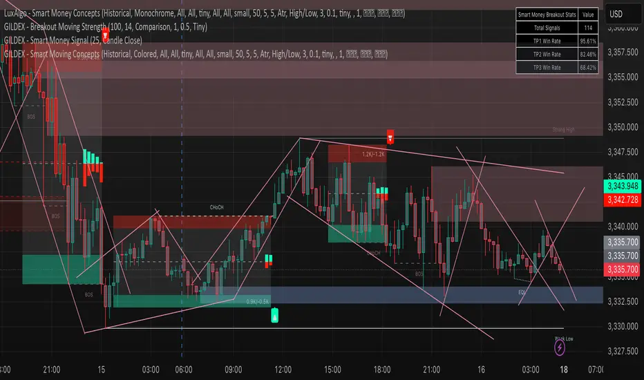
Smart Moving Concepts [GILDEX]This all-in-one indicator displays real-time market structure (internal & swing BOS / CHoCH), order blocks, premium & discount zones, equal highs & lows, and much more...allowing traders to automatically mark up their charts with widely used price action methodologies. Following the release of our Fair Value Gap script, we received numerous requests from our community to release more features in the same category.
"Smart Money Concepts" (SMC) is a fairly new yet widely used term amongst price action traders looking to more accurately navigate liquidity & find more optimal points of interest in the market. Trying to determine where institutional market participants have orders placed (buy or sell side liquidity) can be a very reasonable approach to finding more practical entries & exits based on price action.
The indicator includes alerts for the presence of swing structures and many other relevant conditions.
Features
This indicator includes many features relevant to SMC, these are highlighted below:
Full internal & swing market structure labeling in real-time
Break of Structure (BOS)
Change of Character (CHoCH)
Order Blocks (bullish & bearish)
Equal Highs & Lows
Fair Value Gap Detection
Previous Highs & Lows
Premium & Discount Zones as a range
Options to style the indicator to more easily display these concepts
Settings
Mode: Allows the user to select Historical (default) or Present, which displays only recent data on the chart.
Style: Allows the user to select different styling for the entire indicator between Colored (default) and Monochrome.
Color Candles: Plots candles based on the internal & swing structures from within the indicator on the chart.
Internal Structure: Displays the internal structure labels & dashed lines to represent them. (BOS & CHoCH).
Confluence Filter: Filter non-significant internal structure breakouts.
Swing Structure: Displays the swing structure labels & solid lines on the chart (larger BOS & CHoCH labels).
Swing Points: Displays swing points labels on chart such as HH, HL, LH, LL.
Internal Order Blocks: Enables Internal Order Blocks & allows the user to select how many most recent Internal Order Blocks appear on the chart.
Swing Order Blocks: Enables Swing Order Blocks & allows the user to select how many most recent Swing Order Blocks appear on the chart.
Equal Highs & Lows: Displays EQH/EQL labels on chart for detecting equal highs & lows.
Bars Confirmation: Allows the user to select how many bars are needed to confirm an EQH/EQL symbol on chart.
Fair Value Gaps: Displays boxes to highlight imbalance areas on the chart.
Auto Threshold: Filter out non-significant fair value gaps.
Timeframe: Allows the user to select the timeframe for the Fair Value Gap detection.
Extend FVG: Allows the user to choose how many bars to extend the Fair Value Gap boxes on the chart.
Highs & Lows MTF: Allows the user to display previous highs & lows from daily, weekly, & monthly timeframes as significant levels.
Premium/Discount Zones: Allows the user to display Premium, Discount, and Equilibrium zones on the chart
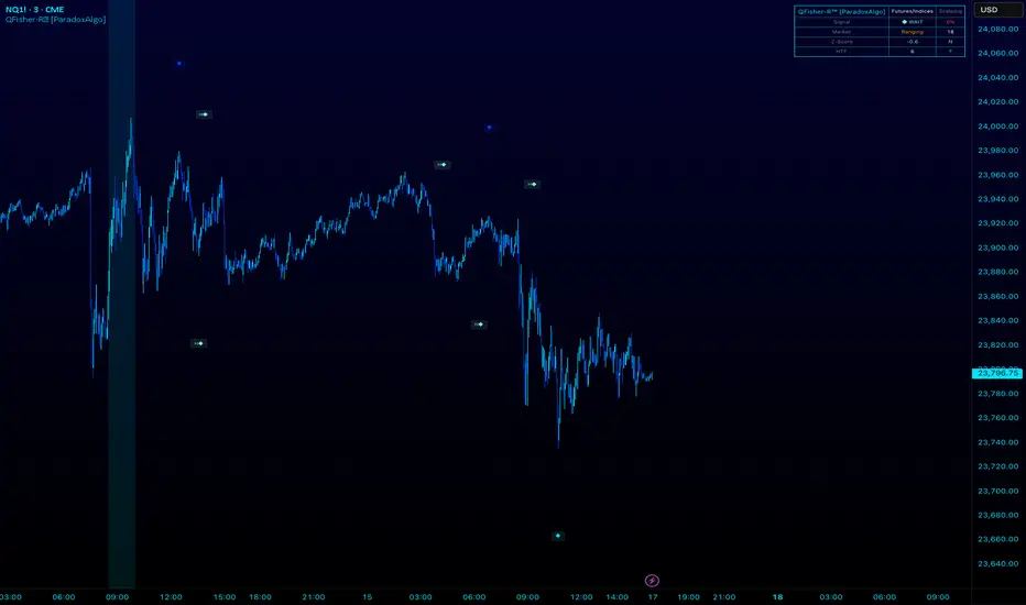
QFisher-R™ [ParadoxAlgo]QFISHER-R™ (Regime-Aware Fisher Transform)
A research/education tool that helps visualize potential momentum exhaustion and probable inflection zones using a quantitative, non-repainting Fisher framework with regime filters and multi-timeframe (MTF) confirmation.
What it does
Converts normalized price movement into a stabilized Fisher domain to highlight potential turning points.
Uses adaptive smoothing, robust (MAD/quantile) thresholds, and optional MTF alignment to contextualize extremes.
Provides a Reversal Probability Score (0–100) to summarize signal confluence (extreme, slope, cross, divergence, regime, and MTF checks).
Key features
Non-repainting logic (bar-close confirmation; security() with no lookahead).
Dynamic exhaustion bands (data-driven thresholds vs fixed ±2).
Adaptive smoothing (efficiency-ratio based).
Optional divergence tags on structurally valid pivots.
MTF confirmation (same logic computed on a higher timeframe).
Compact visuals with subtle plotting to reduce chart clutter.
Inputs (high level)
Source (e.g., HLC3 / Close / HA).
Core lookback, fast/slow range blend, and ER length.
Band sensitivity (robust thresholding).
MTF timeframe(s) and agreement requirement.
Toggle divergence & intrabar previews (default off).
Signals & Alerts
Turn Candidate (Up/Down) when multiple conditions align.
Trade-Grade Turn when score ≥ threshold and MTF agrees.
Divergence Confirmed when structural criteria are met.
Alerts are generated on confirmed bar close by default. Optional “preview” mode is available for experimentation.
How to use
Start on your preferred timeframe; optionally enable an HTF (e.g., 4×) for confirmation.
Look for RPS clusters near the exhaustion bands, slope inflections, and (optionally) divergences.
Combine with your own risk management, liquidity, and trend context.
Paper test first and calibrate thresholds to your instrument and timeframe.
Notes & limitations
This is not a buy/sell signal generator and does not predict future returns.
Readings can remain extreme during strong trends; use HTF context and your own filters.
Parameters are intentionally conservative by default; adjust carefully.
Compliance / Disclaimer
Educational & research tool only. Not financial advice. No recommendation to buy/sell any security or derivative.
Past performance, backtests, or examples (if any) are not indicative of future results.
Trading involves risk; you are responsible for your own decisions and risk management.
Built upon the Fisher Transform concept (Ehlers); all modifications, smoothing, regime logic, scoring, and visualization are original work by Paradox Algo.
Volume Profile Grid [Alpha Extract]A sophisticated volume distribution analysis system that transforms market activity into institutional-grade visual profiles, revealing hidden support/resistance zones and market participant behavior. Utilizing advanced price level segmentation, bullish/bearish volume separation, and dynamic range analysis, the Volume Profile Grid delivers comprehensive market structure insights with Point of Control (POC) identification, Value Area boundaries, and volume delta analysis. The system features intelligent visualization modes, real-time sentiment analysis, and flexible range selection to provide traders with clear, actionable volume-based market context.
🔶 Dynamic Range Analysis Engine
Implements dual-mode range selection with visible chart analysis and fixed period lookback, automatically adjusting to current market view or analyzing specified historical periods. The system intelligently calculates optimal bar counts while maintaining performance through configurable maximum limits, ensuring responsive profile generation across all timeframes with institutional-grade precision.
// Dynamic period calculation with intelligent caching
get_analysis_period() =>
if i_use_visible_range
chart_start_time = chart.left_visible_bar_time
current_time = last_bar_time
time_span = current_time - chart_start_time
tf_seconds = timeframe.in_seconds()
estimated_bars = time_span / (tf_seconds * 1000)
range_bars = math.floor(estimated_bars)
final_bars = math.min(range_bars, i_max_visible_bars)
math.max(final_bars, 50) // Minimum threshold
else
math.max(i_periods, 50)
🔶 Advanced Bull/Bear Volume Separation
Employs sophisticated candle classification algorithms to separate bullish and bearish volume at each price level, with weighted distribution based on bar intersection ratios. The system analyzes open/close relationships to determine volume direction, applying proportional allocation for doji patterns and ensuring accurate representation of buying versus selling pressure across the entire price spectrum.
🔶 Multi-Mode Volume Visualization
Features three distinct display modes for bull/bear volume representation: Split mode creates mirrored profiles from a central axis, Side by Side mode displays sequential bull/bear segments, and Stacked mode separates volumes vertically. Each mode offers unique insights into market participant behavior with customizable width, thickness, and color parameters for optimal visual clarity.
// Bull/Bear volume calculation with weighted distribution
for bar_offset = 0 to actual_periods - 1
bar_high = high
bar_low = low
bar_volume = volume
// Calculate intersection weight
weight = math.min(bar_high, next_level) - math.max(bar_low, current_level)
weight := weight / (bar_high - bar_low)
weighted_volume = bar_volume * weight
// Classify volume direction
if bar_close > bar_open
level_bull_volume += weighted_volume
else if bar_close < bar_open
level_bear_volume += weighted_volume
else // Doji handling
level_bull_volume += weighted_volume * 0.5
level_bear_volume += weighted_volume * 0.5
🔶 Point of Control & Value Area Detection
Implements institutional-standard POC identification by locating the price level with maximum volume accumulation, providing critical support/resistance zones. The Value Area calculation uses sophisticated sorting algorithms to identify the price range containing 70% of trading volume, revealing the market's accepted value zone where institutional participants concentrate their activity.
🔶 Volume Delta Analysis System
Incorporates real-time volume delta calculation with configurable dominance thresholds to identify significant bull/bear imbalances. The system visually highlights price levels where buying or selling pressure exceeds threshold percentages, providing immediate insight into directional volume flow and potential reversal zones through color-coded delta indicators.
// Value Area calculation using 70% volume accumulation
total_volume_sum = array.sum(total_volumes)
target_volume = total_volume_sum * 0.70
// Sort volumes to find highest activity zones
for i = 0 to array.size(sorted_volumes) - 2
for j = i + 1 to array.size(sorted_volumes) - 1
if array.get(sorted_volumes, j) > array.get(sorted_volumes, i)
// Swap and track indices for value area boundaries
// Accumulate until 70% threshold reached
for i = 0 to array.size(sorted_indices) - 1
accumulated_volume += vol
array.push(va_levels, array.get(volume_levels, idx))
if accumulated_volume >= target_volume
break
❓How It Works
🔶 Weighted Volume Distribution
Implements proportional volume allocation based on the percentage of each bar that intersects with price levels. When a bar spans multiple levels, volume is distributed proportionally based on the intersection ratio, ensuring precise representation of trading activity across the entire price spectrum without double-counting or volume loss.
🔶 Real-Time Profile Generation
Profiles regenerate on each bar close when in visible range mode, automatically adapting to chart zoom and scroll actions. The system maintains optimal performance through intelligent caching mechanisms and selective line updates, ensuring smooth operation even with maximum resolution settings and extended analysis periods.
🔶 Market Sentiment Analysis
Features comprehensive volume analysis table displaying total volume metrics, bullish/bearish percentages, and overall market sentiment classification. The system calculates volume dominance ratios in real-time, providing immediate insight into whether buyers or sellers control the current price structure with percentage-based sentiment thresholds.
🔶 Visual Profile Mapping
Provides multi-layered visual feedback through colored volume bars, POC line highlighting, Value Area boundaries, and optional delta indicators. The system supports profile mirroring for alternative perspectives, line extension for future reference, and customizable label positioning with detailed price information at critical levels.
Why Choose Volume Profile Grid
The Volume Profile Grid represents the evolution of volume analysis tools, combining traditional volume profile concepts with modern visualization techniques and intelligent analysis algorithms. By integrating dynamic range selection, sophisticated bull/bear separation, and multi-mode visualization with POC/Value Area detection, it provides traders with institutional-quality market structure analysis that adapts to any trading style. The comprehensive delta analysis and sentiment monitoring system eliminates guesswork while the flexible visualization options ensure optimal clarity across all market conditions, making it an essential tool for traders seeking to understand true market dynamics through volume-based price discovery.

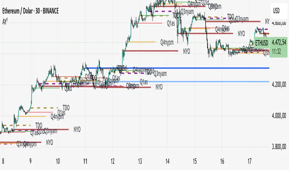
TrueOpens [AY]¹ See how price reacts to key multi-day and monthly open levels—perfect for S/R-focused traders.
Experimental indicator for tracking multi-day openings and ICT True Month Open levels, ideal for S/R traders.
TrueOpens ¹ – Multi-Day & True Month Open Levels
This indicator is experimental and designed to help traders visually track opening price levels across multiple days, along with the ICT True Month Open (TMO).
Key Features:
Supports up to 12 configurable multi-day opening sessions, each with independent color, style, width, and label options.
Automatically detects the True Month Open using the ICT method (2nd Monday of each month) and plots it on the chart.
Lines can extend dynamically and are limited to a user-defined number of historical bars for clarity.
Fully customizable timezones, label sizes, and display options.
This indicator is ideal for observing how price interacts with key levels, especially for traders who favor support and resistance-based strategies.
Disclaimer: This is an analytical tool for observation purposes. It does not provide buy or sell signals. Users should combine it with their own analysis and risk management.
Intraday Spark Chart [AstrideUnicorn]The Intraday Spark Chart (ISC) is a minimalist yet powerful tool designed to track an asset’s performance relative to its daily opening price. Inspired by Nasdaq's trading-floor analog dashboards, it visualizes intraday percentage changes as a color-coded sparkline, helping traders quickly gauge momentum and session bias.
Ideal for: Day trading, scalping, and multi-asset monitoring.
Best paired with: 1m to 4H timeframes (auto-warns on higher TFs).
Key metrics:
Real-time % change from daily open.
Final daily % change (updated at session close).
Daily open price labels for orientation.
HOW TO USE
Visual Guide
Sparkline Plot:
A green area/line indicates price is above the daily open (bullish).
A red area/line signals price is below the daily open (bearish).
The baseline (0%) represents the daily open price.
Session Markers:
The dotted vertical lines separate trading days.
Gray labels near the baseline show the exact daily open price at the start of each session.
Dynamic Labels:
The labels in the upper left corner of each session range display the current (or final) daily % change. Color matches the trend (green/red) for instant readability.
Practical Use Cases
Opening Range Breakouts: Spot early momentum by observing how price reacts to the daily open.
Multi-Asset Screening: Compare intraday strength across symbols by choosing an asset in the indicator settings panel.
Session Close Prep: Anticipate daily settlement by tracking the final % change (useful for futures/swing traders).
SETTINGS
Asset (Input Symbol) : Defaults to the current chart symbol. Choose any asset to monitor its price action without switching charts - ideal for intermarket analysis or correlation tracking.

MA Suite | Lyro RSMA Suite | Lyro RS
Overview
The MA Suite is a versatile moving average visualization tool designed for traders who demand clarity, flexibility, and actionable market signals. With support for over 16 different moving average types, built-in trend detection, dynamic coloring, and optional support/resistance & rejection markers, it transforms the humble MA into a fully-featured decision-making aid.
Key Features
Multi-Type Moving Averages
Choose from 16 MA calculations including SMA, EMA, WMA, VWMA, HMA, LSMA, FRAMA, KAMA, JMA, T3, and more.
Tailor responsiveness vs. smoothness to your strategy.
Trend Logic Modes
Source Above MA – Colors and signals are based on price position relative to the MA.
Rising MA – Colors and signals are determined by MA slope direction.
Support & Resistance Markers
Plots ▲ for potential support touches.
Plots ▼ for potential resistance touches when price interacts with the MA.
Rejection Signals
Flags bullish rejection when price bounces upward after an MA test.
Flags bearish rejection when price reverses downward after an MA test.
Plotted directly on the chart as labeled markers.
Customizable Color Palettes
Select from Classic, Mystic, Accented, or Royal themes.
Define custom bullish/bearish colors for complete visual control.
Glow & Styling Effects
Multi-layer glow lines around the MA enhance visibility.
Keeps charts clean while improving clarity.
How It Works
MA Calculation – Applies the chosen MA type to your selected price source.
Trend Coloring – Colors switch based on price position or MA slope logic.
Support/Resistance Detection – Identifies MA “touch” events with ▲ or ▼ markers.
Rejection Logic – Detects reversals after MA touches, adding bullish/bearish labels.
Practical Use
Trend Following – In “Source Above MA” mode, use color changes and crossovers to confirm bias.
Dynamic S/R – Use ▲ / ▼ markers to identify support or resistance in trending or ranging markets.
Reversal Opportunities – Monitor rejection labels for potential turning points against prevailing trend.
Customization
Select MA type and length to fine-tune indicator behavior.
Switch between trend modes for different trading styles.
Enable or disable S/R and rejection markers.
Personalize visuals with palette selection or custom colors.
⚠️Disclaimer
This indicator is a tool for technical analysis and does not provide guaranteed results. It should be used in conjunction with other analysis methods and proper risk management practices. The creators of this indicator are not responsible for any financial decisions made based on its signals.

Dynamic Support and Resistance V2 | AnonycryptousThe Dynamic Support and Resistance V2 indicator, an easy tool to identify key support, resistance, trendline levels, pivot points and volume data.
Pivot Points.
Calculates support, resistance and trendline levels using pivot points, which are derived from the high, low, and close prices of previous trading periods.
Customize the pivot calculation by using Close' or 'High/Low' and adjusting the lookback periods for both the left and right sides of the pivot calculation.
Pivot points are crucial for forecasting potential market turning points, so it allows traders to adapt the indicator to different market conditions and timeframes.
By using pivot points, traders can spot reversal and consolidation levels or trendlines early on, allowing them to react to them in time.
Volume Levels.
This option focuses on identifying support and resistance levels based on volume data, specifically the Point of Control.
The POC is the highest traded volume price level during a time period.
This POC calculation, allow traders to areas of significant trading levels as support or resistance zones.
Volume-based levels gives insights into market sentiment and showes strong support and resistance based on trading volume.
Traders can choose between pivot-based and volume-based levels or use both simultaneously, depending on their analysis.
The indicator offers custom colors, so the trader can customize their visual analysis to their own style.
It calculates the importance of each level based on the number of touches and the duration it holds.
This indicator is intended for educational and informational purposes only and should not be considered financial advice.
Trading involves significant risk, and you should consult with a financial advisor before making any trading decisions.
The performance of this indicator is not guaranteed, and past results do not predict future performance.
Use at your own risk.
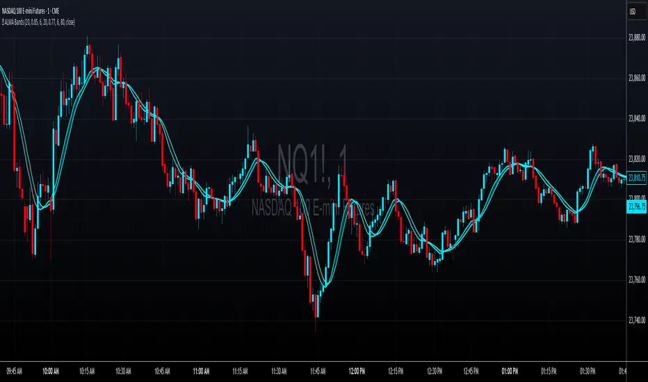
🌊 ALMA BandsTrend Architect Suite Lite - ALMA Bands - Adaptive Moving Average System
Simple implementation of ALMA (Arnaud Legoux Moving Average) bands from the Trend Architect Suite.
Why ALMA over Traditional EMA Bands?
Superior Smoothness: ALMA combines the best of both SMA and EMA by using Gaussian filters to reduce noise while maintaining responsiveness
Reduced Lag: The offset parameter allows fine-tuning between minimal lag and maximum smoothness
Advanced Weighting: Uses a sophisticated weighted algorithm that reduces false signals compared to traditional moving averages
Configurable Phase: The offset parameter (0-1) controls the phase shift, allowing you to balance between smoothness and responsiveness
Features:
Dual ALMA lines with customizable periods, offsets, and sigma values
Dynamic fill coloring (cyan for bullish, red for bearish trends)
Clean crossover alerts for trend changes
Fully customizable appearance and sensitivity
Settings:
Default configuration uses 20-period ALMAs with different offset values (0.85 vs 0.77)
All parameters are adjustable to fit your trading style
Use Case:
Trend-following system suitable for any timeframe. Best used in conjunction with other analysis for confirmation.
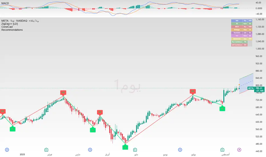
Recommendation Indicatorالوصف بالعربية
استراتيجية تداول مبنية على ٦ مؤشرات تأكيدية لرصد حركة السوق واتجاهه.
تعتمد على عدّ الشموع الصاعدة والهابطة المتتالية كعامل أساسي، وتدمج معها مؤشرات إضافية للتأكيد.
عند توافق المؤشرات معًا، يتم توليد إشارة شراء (BUY) أو بيع (SELL) واضحة على الرسم البياني.
هذا يعزز دقة الإشارات ويقلل من التذبذبات أو الإشارات الكاذبة، مما يجعلها مناسبة للمتداولين الباحثين عن قوة الاتجاه وتأكيده قبل الدخول في الصفقة.
🔎 ملاحظات الاستخدام
الاستراتيجية تحتوي على ٦ أدوات تأكيد مجتمعة لضمان إشارات أدق.
يُفضل استخدامها مع اختبار رجعي (Backtesting) قبل التداول الفعلي.
يمكن تعديل إعدادات المؤشرات لتناسب السوق أو الإطار الزمني المستخدم.
لا تعتبر توصية مالية مباشرة، وإنما أداة تعليمية وتجريبية.
---
📌 Description in English
A trading strategy built on 6 confirmation indicators to track market movements and trends.
It uses consecutive up and down bars as the core logic, combined with additional indicators for confirmation.
When all confirmations align, the strategy generates clear BUY or SELL signals on the chart.
This approach improves signal accuracy, reduces noise, and helps traders confirm market direction before entering a trade.
🔎 Usage Notes
The strategy incorporates 6 confirmation tools working together for higher accuracy.
Backtesting is recommended before applying it to live trading.
Indicator parameters can be adjusted to fit different markets and timeframes.
This is not financial advice, but an educational and experimental tool.
Body & Volume-Based Buy/Sell Signals (5min 1.5M Vol)Only for 5 min and Volume 1.5M
Conditions (Summarized)
🔹 BUY Signal
Previous candle is red: close < open
Current candle is green: close > open
Previous candle body is smaller than current:
abs(close - open ) < abs(close - open)
Previous candle body size ≥ 10 points
Both candles' volume ≥ minVolume (default: 2,000,000)
➜ Plot BUY below green candle
🔸 SELL Signal
Previous candle is green: close > open
Current candle is red: close < open
Previous candle body is smaller than current:
abs(close - open ) < abs(close - open)
Previous candle body size ≥ 10 points
Both candles' volume ≥ minVolume
➜ Plot SELL above red candle

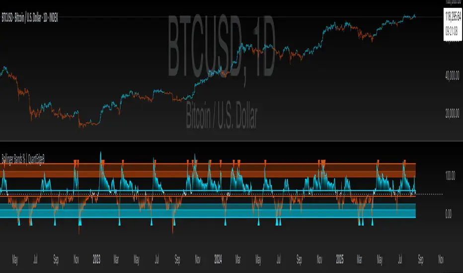
Bollinger Bands % | QuantEdgeB📊 Introducing Bollinger Bands % (BB%) by QuantEdgeB
🛠️ Overview
BB% | QuantEdgeB is a volatility-aware momentum tool that maps price within a Bollinger envelope onto a normalized scale. By letting you choose the base moving average (SMA, EMA, DEMA, TEMA, HMA, ALMA, EHMA, THMA, RMA, WMA, VWMA, T3, LSMA) and even Heikin-Ashi sources, it adapts to your style while keeping readings consistent across symbols and timeframes. Clear thresholds and color-coded visuals make it easy to spot emerging strength, fading moves, and potential mean-reversions.
✨ Key Features
• 🔹 Flexible Baseline
Pick from 12 MA types (plus Heikin-Ashi source option) to tailor responsiveness and smoothness.
• 🔹 Normalized Positioning
Price is expressed as a percentage of the band range, yielding an intuitive 0–100 style read (can exceed in extreme trends).
• 🔹 Actionable Thresholds
Default Long 55 / Short 45 levels provide simple, objective triggers.
• 🔹 Visual Clarity
Color-coded candles, shaded OB/OS zones, and adaptive color themes speed up decision-making.
• 🔹 Ready-to-Alert
Built-in alerts for long/short transitions.
📐 How It Works
1️⃣ Band Construction
A moving average (your choice) defines the midline; volatility (standard deviation) builds upper/lower bands.
2️⃣ Normalization
The indicator measures where price sits between the lower and upper band, scaling that into a bounded oscillator (BB%).
3️⃣ Signal Logic
• ✅ Long when BB% rises above 55 (strength toward the top of the envelope).
• ❌ Short when BB% falls below 45 (weakness toward the bottom).
4️⃣ OB/OS Context
Shaded regions above/below typical ranges highlight exhaustion and potential snap-backs.
⚙️ Custom Settings
• Base MA Type: SMA, EMA, DEMA, TEMA, HMA, ALMA, EHMA, THMA, RMA, WMA, VWMA, T3, LSMA
• Source Mode: Classic price or Heikin-Ashi (close/open/high/hlc3)
• Base Length: default 40
• Band Width: standard deviation-based (2× SD by default)
• Long / Short Thresholds: defaults 55 / 45
• Color Mode: Alpha, MultiEdge, TradingSuite, Premium, Fundamental, Classic, Warm, Cold, Strategy
• Candles & Labels: optional candle coloring and signal markers
👥 Ideal For
✅ Trend Followers — Ride strength as price compresses near the upper band.
✅ Swing/Mean-Reversion Traders — Fade extremes when BB% stretches into OB/OS zones.
✅ Multi-Timeframe Analysts — Compare band position consistently across periods.
✅ System Builders — Use BB% as a normalized feature for strategies and filters.
📌 Conclusion
BB% | QuantEdgeB delivers a clean, normalized read of price versus its volatility envelope—adaptable via rich MA/source options and easy to automate with thresholds and alerts.
🔹 Key Takeaways:
1️⃣ Normalized view of price inside the volatility bands
2️⃣ Flexible baseline (12+ MA choices) and Heikin-Ashi support
3️⃣ Straightforward 55/45 triggers with clear visual context
📌 Disclaimer: Past performance is not indicative of future results. No strategy guarantees success.
📌 Strategic Advice: Always backtest, tune parameters, and align with your risk profile before live trading.
Leg Out Candle V2.0The Script marks candles that could be considered as a leg out of a supply/demand and are bigger than the previous ones based on the adjustable lookback value. There is also the option to adjust the threshold ob the body to wick ratio of the leg out candle. The lowest value is 50% because anything lower would be a basing candle.

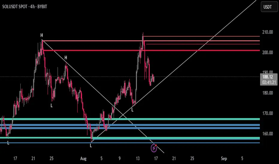
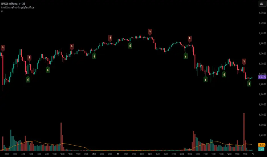
Market Structure Trend Change by TenAMTraderMarket Structure Trend Change Indicator
Description:
This indicator detects changes in market trend by analyzing swing highs and lows to identify Higher Highs (HH), Higher Lows (HL), Lower Highs (LH), and Lower Lows (LL). It helps traders quickly see potential reversals and trend continuation points.
Features:
Automatically identifies pivots based on configurable left and right bars.
Labels pivot points (HH, HL, LH, LL) directly on the chart (text-only for clarity).
Generates buy and sell signals when a trend change is detected:
Buy Signal: HL after repeated LLs.
Sell Signal: LH after repeated HHs.
Fully customizable signal appearance: arrow type, circle, label, color, and size.
Adjustable minimum number of repeated highs or lows before a trend change triggers a signal.
Alerts built in for automated notifications when buy/sell signals occur.
Default Settings:
Optimized for a 10-minute chart.
Default “Min repeats before trend change” and pivot left/right bars are set for typical 10-min price swings.
User Customization:
Adjust the “Pivot Left Bars,” “Pivot Right Bars,” and “Min repeats before trend change” to match your trading style, chart timeframe, and volatility.
Enable pivot labels for visual clarity if desired.
Set alerts to receive notifications of trend changes in real time.
How to Use:
Apply the indicator to any chart and timeframe. It works best on swing-trading or trend-following strategies.
Watch for Buy/Sell signals in conjunction with your other analysis, such as volume, support/resistance, or other indicators.
Legal Disclaimer:
This indicator is provided for educational and informational purposes only. It is not financial advice. Trading involves substantial risk, and past performance is not indicative of future results. Users should trade at their own risk and are solely responsible for any gains or losses incurred.
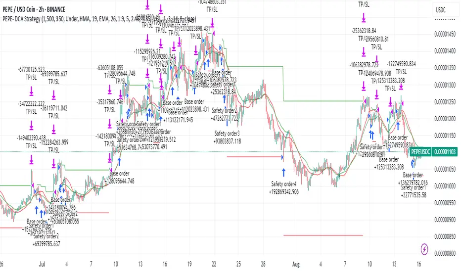
DCA Strategy on Steroids for CryptoThis strategy getting only in Long position for Crypto
Using Fast and Slow moving Averages and Stochastic RSI to get in Long position
Fast and Slow moving Averages - cross-under - I Prefer - or opposite for Bull Market
Stochastic RSI cross-over - 5 and Trend Determined by the Fast moving Average
There is no Stop loss is not for one with small tolerance to getting under
Fast and Slow moving Averages and Stochastic RSI Parameters can be adjust
The bot Use Safe Trades and Price Deviation Determined from the User
Max Safe Trades = 10
Take profit Parameters can be adjust in %
Pepe-USDC is just a example What the bot Can do
EMA + MACD + RSI Strategy"This strategy combines EMA crossovers (20/50), MACD momentum (12/26/9), and RSI thresholds (14-period) to generate signals. It triggers a BUY when:
EMA20 crosses above EMA50,
MACD line > Signal line,
RSI > 50.
SELL signals activate on the opposite conditions. Visual alerts plot directly on the chart

PP_Solstice StrategyThis strategy was developed by Vinay with inputs from Warren, Dodgie and others to replicate TOS AGAIG indicators. It is available for free of use.

Markov Chain [3D] | FractalystWhat exactly is a Markov Chain?
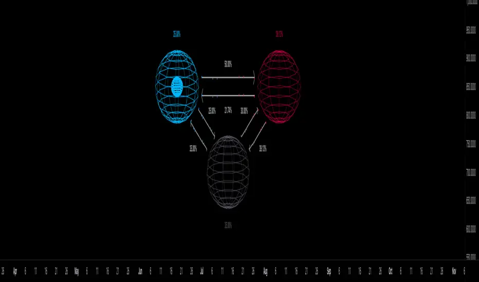
This indicator uses a Markov Chain model to analyze, quantify, and visualize the transitions between market regimes (Bull, Bear, Neutral) on your chart. It dynamically detects these regimes in real-time, calculates transition probabilities, and displays them as animated 3D spheres and arrows, giving traders intuitive insight into current and future market conditions.
How does a Markov Chain work, and how should I read this spheres-and-arrows diagram?
Think of three weather modes: Sunny, Rainy, Cloudy.
Each sphere is one mode. The loop on a sphere means “stay the same next step” (e.g., Sunny again tomorrow).
The arrows leaving a sphere show where things usually go next if they change (e.g., Sunny moving to Cloudy).
Some paths matter more than others. A more prominent loop means the current mode tends to persist. A more prominent outgoing arrow means a change to that destination is the usual next step.
Direction isn’t symmetric: moving Sunny→Cloudy can behave differently than Cloudy→Sunny.
Now relabel the spheres to markets: Bull, Bear, Neutral.
Spheres: market regimes (uptrend, downtrend, range).
Self‑loop: tendency for the current regime to continue on the next bar.
Arrows: the most common next regime if a switch happens.
How to read: Start at the sphere that matches current bar state. If the loop stands out, expect continuation. If one outgoing path stands out, that switch is the typical next step. Opposite directions can differ (Bear→Neutral doesn’t have to match Neutral→Bear).
What states and transitions are shown?
The three market states visualized are:
Bullish (Bull): Upward or strong-market regime.
Bearish (Bear): Downward or weak-market regime.
Neutral: Sideways or range-bound regime.
Bidirectional animated arrows and probability labels show how likely the market is to move from one regime to another (e.g., Bull → Bear or Neutral → Bull).
How does the regime detection system work?
You can use either built-in price returns (based on adaptive Z-score normalization) or supply three custom indicators (such as volume, oscillators, etc.).
Values are statistically normalized (Z-scored) over a configurable lookback period.
The normalized outputs are classified into Bull, Bear, or Neutral zones.
If using three indicators, their regime signals are averaged and smoothed for robustness.
How are transition probabilities calculated?
On every confirmed bar, the algorithm tracks the sequence of detected market states, then builds a rolling window of transitions.
The code maintains a transition count matrix for all regime pairs (e.g., Bull → Bear).
Transition probabilities are extracted for each possible state change using Laplace smoothing for numerical stability, and frequently updated in real-time.
What is unique about the visualization?
3D animated spheres represent each regime and change visually when active.
Animated, bidirectional arrows reveal transition probabilities and allow you to see both dominant and less likely regime flows.
Particles (moving dots) animate along the arrows, enhancing the perception of regime flow direction and speed.
All elements dynamically update with each new price bar, providing a live market map in an intuitive, engaging format.
Can I use custom indicators for regime classification?
Yes! Enable the "Custom Indicators" switch and select any three chart series as inputs. These will be normalized and combined (each with equal weight), broadening the regime classification beyond just price-based movement.
What does the “Lookback Period” control?
Lookback Period (default: 100) sets how much historical data builds the probability matrix. Shorter periods adapt faster to regime changes but may be noisier. Longer periods are more stable but slower to adapt.
How is this different from a Hidden Markov Model (HMM)?
It sets the window for both regime detection and probability calculations. Lower values make the system more reactive, but potentially noisier. Higher values smooth estimates and make the system more robust.
How is this Markov Chain different from a Hidden Markov Model (HMM)?
Markov Chain (as here): All market regimes (Bull, Bear, Neutral) are directly observable on the chart. The transition matrix is built from actual detected regimes, keeping the model simple and interpretable.
Hidden Markov Model: The actual regimes are unobservable ("hidden") and must be inferred from market output or indicator "emissions" using statistical learning algorithms. HMMs are more complex, can capture more subtle structure, but are harder to visualize and require additional machine learning steps for training.
A standard Markov Chain models transitions between observable states using a simple transition matrix, while a Hidden Markov Model assumes the true states are hidden (latent) and must be inferred from observable “emissions” like price or volume data. In practical terms, a Markov Chain is transparent and easier to implement and interpret; an HMM is more expressive but requires statistical inference to estimate hidden states from data.
Markov Chain: states are observable; you directly count or estimate transition probabilities between visible states. This makes it simpler, faster, and easier to validate and tune.
HMM: states are hidden; you only observe emissions generated by those latent states. Learning involves machine learning/statistical algorithms (commonly Baum–Welch/EM for training and Viterbi for decoding) to infer both the transition dynamics and the most likely hidden state sequence from data.
How does the indicator avoid “repainting” or look-ahead bias?
All regime changes and matrix updates happen only on confirmed (closed) bars, so no future data is leaked, ensuring reliable real-time operation.
Are there practical tuning tips?
Tune the Lookback Period for your asset/timeframe: shorter for fast markets, longer for stability.
Use custom indicators if your asset has unique regime drivers.
Watch for rapid changes in transition probabilities as early warning of a possible regime shift.
Who is this indicator for?
Quants and quantitative researchers exploring probabilistic market modeling, especially those interested in regime-switching dynamics and Markov models.
Programmers and system developers who need a probabilistic regime filter for systematic and algorithmic backtesting:
The Markov Chain indicator is ideally suited for programmatic integration via its bias output (1 = Bull, 0 = Neutral, -1 = Bear).
Although the visualization is engaging, the core output is designed for automated, rules-based workflows—not for discretionary/manual trading decisions.
Developers can connect the indicator’s output directly to their Pine Script logic (using input.source()), allowing rapid and robust backtesting of regime-based strategies.
It acts as a plug-and-play regime filter: simply plug the bias output into your entry/exit logic, and you have a scientifically robust, probabilistically-derived signal for filtering, timing, position sizing, or risk regimes.
The MC's output is intentionally "trinary" (1/0/-1), focusing on clear regime states for unambiguous decision-making in code. If you require nuanced, multi-probability or soft-label state vectors, consider expanding the indicator or stacking it with a probability-weighted logic layer in your scripting.
Because it avoids subjectivity, this approach is optimal for systematic quants, algo developers building backtested, repeatable strategies based on probabilistic regime analysis.
What's the mathematical foundation behind this?
The mathematical foundation behind this Markov Chain indicator—and probabilistic regime detection in finance—draws from two principal models: the (standard) Markov Chain and the Hidden Markov Model (HMM).
How to use this indicator programmatically?
The Markov Chain indicator automatically exports a bias value (+1 for Bullish, -1 for Bearish, 0 for Neutral) as a plot visible in the Data Window. This allows you to integrate its regime signal into your own scripts and strategies for backtesting, automation, or live trading.
Step-by-Step Integration with Pine Script (input.source)
Add the Markov Chain indicator to your chart.
This must be done first, since your custom script will "pull" the bias signal from the indicator's plot.
In your strategy, create an input using input.source()
Example:
//@version=5
strategy("MC Bias Strategy Example")
mcBias = input.source(close, "MC Bias Source")
After saving, go to your script’s settings. For the “MC Bias Source” input, select the plot/output of the Markov Chain indicator (typically its bias plot).
Use the bias in your trading logic
Example (long only on Bull, flat otherwise):
if mcBias == 1
strategy.entry("Long", strategy.long)
else
strategy.close("Long")
For more advanced workflows, combine mcBias with additional filters or trailing stops.
How does this work behind-the-scenes?
TradingView’s input.source() lets you use any plot from another indicator as a real-time, “live” data feed in your own script (source).
The selected bias signal is available to your Pine code as a variable, enabling logical decisions based on regime (trend-following, mean-reversion, etc.).
This enables powerful strategy modularity : decouple regime detection from entry/exit logic, allowing fast experimentation without rewriting core signal code.
Integrating 45+ Indicators with Your Markov Chain — How & Why
The Enhanced Custom Indicators Export script exports a massive suite of over 45 technical indicators—ranging from classic momentum (RSI, MACD, Stochastic, etc.) to trend, volume, volatility, and oscillator tools—all pre-calculated, centered/scaled, and available as plots.
// Enhanced Custom Indicators Export - 45 Technical Indicators
// Comprehensive technical analysis suite for advanced market regime detection
//@version=6
indicator('Enhanced Custom Indicators Export | Fractalyst', shorttitle='Enhanced CI Export', overlay=false, scale=scale.right, max_labels_count=500, max_lines_count=500)
// |----- Input Parameters -----| //
momentum_group = "Momentum Indicators"
trend_group = "Trend Indicators"
volume_group = "Volume Indicators"
volatility_group = "Volatility Indicators"
oscillator_group = "Oscillator Indicators"
display_group = "Display Settings"
// Common lengths
length_14 = input.int(14, "Standard Length (14)", minval=1, maxval=100, group=momentum_group)
length_20 = input.int(20, "Medium Length (20)", minval=1, maxval=200, group=trend_group)
length_50 = input.int(50, "Long Length (50)", minval=1, maxval=200, group=trend_group)
// Display options
show_table = input.bool(true, "Show Values Table", group=display_group)
table_size = input.string("Small", "Table Size", options= , group=display_group)
// |----- MOMENTUM INDICATORS (15 indicators) -----| //
// 1. RSI (Relative Strength Index)
rsi_14 = ta.rsi(close, length_14)
rsi_centered = rsi_14 - 50
// 2. Stochastic Oscillator
stoch_k = ta.stoch(close, high, low, length_14)
stoch_d = ta.sma(stoch_k, 3)
stoch_centered = stoch_k - 50
// 3. Williams %R
williams_r = ta.stoch(close, high, low, length_14) - 100
// 4. MACD (Moving Average Convergence Divergence)
= ta.macd(close, 12, 26, 9)
// 5. Momentum (Rate of Change)
momentum = ta.mom(close, length_14)
momentum_pct = (momentum / close ) * 100
// 6. Rate of Change (ROC)
roc = ta.roc(close, length_14)
// 7. Commodity Channel Index (CCI)
cci = ta.cci(close, length_20)
// 8. Money Flow Index (MFI)
mfi = ta.mfi(close, length_14)
mfi_centered = mfi - 50
// 9. Awesome Oscillator (AO)
ao = ta.sma(hl2, 5) - ta.sma(hl2, 34)
// 10. Accelerator Oscillator (AC)
ac = ao - ta.sma(ao, 5)
// 11. Chande Momentum Oscillator (CMO)
cmo = ta.cmo(close, length_14)
// 12. Detrended Price Oscillator (DPO)
dpo = close - ta.sma(close, length_20)
// 13. Price Oscillator (PPO)
ppo = ta.sma(close, 12) - ta.sma(close, 26)
ppo_pct = (ppo / ta.sma(close, 26)) * 100
// 14. TRIX
trix_ema1 = ta.ema(close, length_14)
trix_ema2 = ta.ema(trix_ema1, length_14)
trix_ema3 = ta.ema(trix_ema2, length_14)
trix = ta.roc(trix_ema3, 1) * 10000
// 15. Klinger Oscillator
klinger = ta.ema(volume * (high + low + close) / 3, 34) - ta.ema(volume * (high + low + close) / 3, 55)
// 16. Fisher Transform
fisher_hl2 = 0.5 * (hl2 - ta.lowest(hl2, 10)) / (ta.highest(hl2, 10) - ta.lowest(hl2, 10)) - 0.25
fisher = 0.5 * math.log((1 + fisher_hl2) / (1 - fisher_hl2))
// 17. Stochastic RSI
stoch_rsi = ta.stoch(rsi_14, rsi_14, rsi_14, length_14)
stoch_rsi_centered = stoch_rsi - 50
// 18. Relative Vigor Index (RVI)
rvi_num = ta.swma(close - open)
rvi_den = ta.swma(high - low)
rvi = rvi_den != 0 ? rvi_num / rvi_den : 0
// 19. Balance of Power (BOP)
bop = (close - open) / (high - low)
// |----- TREND INDICATORS (10 indicators) -----| //
// 20. Simple Moving Average Momentum
sma_20 = ta.sma(close, length_20)
sma_momentum = ((close - sma_20) / sma_20) * 100
// 21. Exponential Moving Average Momentum
ema_20 = ta.ema(close, length_20)
ema_momentum = ((close - ema_20) / ema_20) * 100
// 22. Parabolic SAR
sar = ta.sar(0.02, 0.02, 0.2)
sar_trend = close > sar ? 1 : -1
// 23. Linear Regression Slope
lr_slope = ta.linreg(close, length_20, 0) - ta.linreg(close, length_20, 1)
// 24. Moving Average Convergence (MAC)
mac = ta.sma(close, 10) - ta.sma(close, 30)
// 25. Trend Intensity Index (TII)
tii_sum = 0.0
for i = 1 to length_20
tii_sum += close > close ? 1 : 0
tii = (tii_sum / length_20) * 100
// 26. Ichimoku Cloud Components
ichimoku_tenkan = (ta.highest(high, 9) + ta.lowest(low, 9)) / 2
ichimoku_kijun = (ta.highest(high, 26) + ta.lowest(low, 26)) / 2
ichimoku_signal = ichimoku_tenkan > ichimoku_kijun ? 1 : -1
// 27. MESA Adaptive Moving Average (MAMA)
mama_alpha = 2.0 / (length_20 + 1)
mama = ta.ema(close, length_20)
mama_momentum = ((close - mama) / mama) * 100
// 28. Zero Lag Exponential Moving Average (ZLEMA)
zlema_lag = math.round((length_20 - 1) / 2)
zlema_data = close + (close - close )
zlema = ta.ema(zlema_data, length_20)
zlema_momentum = ((close - zlema) / zlema) * 100
// |----- VOLUME INDICATORS (6 indicators) -----| //
// 29. On-Balance Volume (OBV)
obv = ta.obv
// 30. Volume Rate of Change (VROC)
vroc = ta.roc(volume, length_14)
// 31. Price Volume Trend (PVT)
pvt = ta.pvt
// 32. Negative Volume Index (NVI)
nvi = 0.0
nvi := volume < volume ? nvi + ((close - close ) / close ) * nvi : nvi
// 33. Positive Volume Index (PVI)
pvi = 0.0
pvi := volume > volume ? pvi + ((close - close ) / close ) * pvi : pvi
// 34. Volume Oscillator
vol_osc = ta.sma(volume, 5) - ta.sma(volume, 10)
// 35. Ease of Movement (EOM)
eom_distance = high - low
eom_box_height = volume / 1000000
eom = eom_box_height != 0 ? eom_distance / eom_box_height : 0
eom_sma = ta.sma(eom, length_14)
// 36. Force Index
force_index = volume * (close - close )
force_index_sma = ta.sma(force_index, length_14)
// |----- VOLATILITY INDICATORS (10 indicators) -----| //
// 37. Average True Range (ATR)
atr = ta.atr(length_14)
atr_pct = (atr / close) * 100
// 38. Bollinger Bands Position
bb_basis = ta.sma(close, length_20)
bb_dev = 2.0 * ta.stdev(close, length_20)
bb_upper = bb_basis + bb_dev
bb_lower = bb_basis - bb_dev
bb_position = bb_dev != 0 ? (close - bb_basis) / bb_dev : 0
bb_width = bb_dev != 0 ? (bb_upper - bb_lower) / bb_basis * 100 : 0
// 39. Keltner Channels Position
kc_basis = ta.ema(close, length_20)
kc_range = ta.ema(ta.tr, length_20)
kc_upper = kc_basis + (2.0 * kc_range)
kc_lower = kc_basis - (2.0 * kc_range)
kc_position = kc_range != 0 ? (close - kc_basis) / kc_range : 0
// 40. Donchian Channels Position
dc_upper = ta.highest(high, length_20)
dc_lower = ta.lowest(low, length_20)
dc_basis = (dc_upper + dc_lower) / 2
dc_position = (dc_upper - dc_lower) != 0 ? (close - dc_basis) / (dc_upper - dc_lower) : 0
// 41. Standard Deviation
std_dev = ta.stdev(close, length_20)
std_dev_pct = (std_dev / close) * 100
// 42. Relative Volatility Index (RVI)
rvi_up = ta.stdev(close > close ? close : 0, length_14)
rvi_down = ta.stdev(close < close ? close : 0, length_14)
rvi_total = rvi_up + rvi_down
rvi_volatility = rvi_total != 0 ? (rvi_up / rvi_total) * 100 : 50
// 43. Historical Volatility
hv_returns = math.log(close / close )
hv = ta.stdev(hv_returns, length_20) * math.sqrt(252) * 100
// 44. Garman-Klass Volatility
gk_vol = math.log(high/low) * math.log(high/low) - (2*math.log(2)-1) * math.log(close/open) * math.log(close/open)
gk_volatility = math.sqrt(ta.sma(gk_vol, length_20)) * 100
// 45. Parkinson Volatility
park_vol = math.log(high/low) * math.log(high/low)
parkinson = math.sqrt(ta.sma(park_vol, length_20) / (4 * math.log(2))) * 100
// 46. Rogers-Satchell Volatility
rs_vol = math.log(high/close) * math.log(high/open) + math.log(low/close) * math.log(low/open)
rogers_satchell = math.sqrt(ta.sma(rs_vol, length_20)) * 100
// |----- OSCILLATOR INDICATORS (5 indicators) -----| //
// 47. Elder Ray Index
elder_bull = high - ta.ema(close, 13)
elder_bear = low - ta.ema(close, 13)
elder_power = elder_bull + elder_bear
// 48. Schaff Trend Cycle (STC)
stc_macd = ta.ema(close, 23) - ta.ema(close, 50)
stc_k = ta.stoch(stc_macd, stc_macd, stc_macd, 10)
stc_d = ta.ema(stc_k, 3)
stc = ta.stoch(stc_d, stc_d, stc_d, 10)
// 49. Coppock Curve
coppock_roc1 = ta.roc(close, 14)
coppock_roc2 = ta.roc(close, 11)
coppock = ta.wma(coppock_roc1 + coppock_roc2, 10)
// 50. Know Sure Thing (KST)
kst_roc1 = ta.roc(close, 10)
kst_roc2 = ta.roc(close, 15)
kst_roc3 = ta.roc(close, 20)
kst_roc4 = ta.roc(close, 30)
kst = ta.sma(kst_roc1, 10) + 2*ta.sma(kst_roc2, 10) + 3*ta.sma(kst_roc3, 10) + 4*ta.sma(kst_roc4, 15)
// 51. Percentage Price Oscillator (PPO)
ppo_line = ((ta.ema(close, 12) - ta.ema(close, 26)) / ta.ema(close, 26)) * 100
ppo_signal = ta.ema(ppo_line, 9)
ppo_histogram = ppo_line - ppo_signal
// |----- PLOT MAIN INDICATORS -----| //
// Plot key momentum indicators
plot(rsi_centered, title="01_RSI_Centered", color=color.purple, linewidth=1)
plot(stoch_centered, title="02_Stoch_Centered", color=color.blue, linewidth=1)
plot(williams_r, title="03_Williams_R", color=color.red, linewidth=1)
plot(macd_histogram, title="04_MACD_Histogram", color=color.orange, linewidth=1)
plot(cci, title="05_CCI", color=color.green, linewidth=1)
// Plot trend indicators
plot(sma_momentum, title="06_SMA_Momentum", color=color.navy, linewidth=1)
plot(ema_momentum, title="07_EMA_Momentum", color=color.maroon, linewidth=1)
plot(sar_trend, title="08_SAR_Trend", color=color.teal, linewidth=1)
plot(lr_slope, title="09_LR_Slope", color=color.lime, linewidth=1)
plot(mac, title="10_MAC", color=color.fuchsia, linewidth=1)
// Plot volatility indicators
plot(atr_pct, title="11_ATR_Pct", color=color.yellow, linewidth=1)
plot(bb_position, title="12_BB_Position", color=color.aqua, linewidth=1)
plot(kc_position, title="13_KC_Position", color=color.olive, linewidth=1)
plot(std_dev_pct, title="14_StdDev_Pct", color=color.silver, linewidth=1)
plot(bb_width, title="15_BB_Width", color=color.gray, linewidth=1)
// Plot volume indicators
plot(vroc, title="16_VROC", color=color.blue, linewidth=1)
plot(eom_sma, title="17_EOM", color=color.red, linewidth=1)
plot(vol_osc, title="18_Vol_Osc", color=color.green, linewidth=1)
plot(force_index_sma, title="19_Force_Index", color=color.orange, linewidth=1)
plot(obv, title="20_OBV", color=color.purple, linewidth=1)
// Plot additional oscillators
plot(ao, title="21_Awesome_Osc", color=color.navy, linewidth=1)
plot(cmo, title="22_CMO", color=color.maroon, linewidth=1)
plot(dpo, title="23_DPO", color=color.teal, linewidth=1)
plot(trix, title="24_TRIX", color=color.lime, linewidth=1)
plot(fisher, title="25_Fisher", color=color.fuchsia, linewidth=1)
// Plot more momentum indicators
plot(mfi_centered, title="26_MFI_Centered", color=color.yellow, linewidth=1)
plot(ac, title="27_AC", color=color.aqua, linewidth=1)
plot(ppo_pct, title="28_PPO_Pct", color=color.olive, linewidth=1)
plot(stoch_rsi_centered, title="29_StochRSI_Centered", color=color.silver, linewidth=1)
plot(klinger, title="30_Klinger", color=color.gray, linewidth=1)
// Plot trend continuation
plot(tii, title="31_TII", color=color.blue, linewidth=1)
plot(ichimoku_signal, title="32_Ichimoku_Signal", color=color.red, linewidth=1)
plot(mama_momentum, title="33_MAMA_Momentum", color=color.green, linewidth=1)
plot(zlema_momentum, title="34_ZLEMA_Momentum", color=color.orange, linewidth=1)
plot(bop, title="35_BOP", color=color.purple, linewidth=1)
// Plot volume continuation
plot(nvi, title="36_NVI", color=color.navy, linewidth=1)
plot(pvi, title="37_PVI", color=color.maroon, linewidth=1)
plot(momentum_pct, title="38_Momentum_Pct", color=color.teal, linewidth=1)
plot(roc, title="39_ROC", color=color.lime, linewidth=1)
plot(rvi, title="40_RVI", color=color.fuchsia, linewidth=1)
// Plot volatility continuation
plot(dc_position, title="41_DC_Position", color=color.yellow, linewidth=1)
plot(rvi_volatility, title="42_RVI_Volatility", color=color.aqua, linewidth=1)
plot(hv, title="43_Historical_Vol", color=color.olive, linewidth=1)
plot(gk_volatility, title="44_GK_Volatility", color=color.silver, linewidth=1)
plot(parkinson, title="45_Parkinson_Vol", color=color.gray, linewidth=1)
// Plot final oscillators
plot(rogers_satchell, title="46_RS_Volatility", color=color.blue, linewidth=1)
plot(elder_power, title="47_Elder_Power", color=color.red, linewidth=1)
plot(stc, title="48_STC", color=color.green, linewidth=1)
plot(coppock, title="49_Coppock", color=color.orange, linewidth=1)
plot(kst, title="50_KST", color=color.purple, linewidth=1)
// Plot final indicators
plot(ppo_histogram, title="51_PPO_Histogram", color=color.navy, linewidth=1)
plot(pvt, title="52_PVT", color=color.maroon, linewidth=1)
// |----- Reference Lines -----| //
hline(0, "Zero Line", color=color.gray, linestyle=hline.style_dashed, linewidth=1)
hline(50, "Midline", color=color.gray, linestyle=hline.style_dotted, linewidth=1)
hline(-50, "Lower Midline", color=color.gray, linestyle=hline.style_dotted, linewidth=1)
hline(25, "Upper Threshold", color=color.gray, linestyle=hline.style_dotted, linewidth=1)
hline(-25, "Lower Threshold", color=color.gray, linestyle=hline.style_dotted, linewidth=1)
// |----- Enhanced Information Table -----| //
if show_table and barstate.islast
table_position = position.top_right
table_text_size = table_size == "Tiny" ? size.tiny : table_size == "Small" ? size.small : size.normal
var table info_table = table.new(table_position, 3, 18, bgcolor=color.new(color.white, 85), border_width=1, border_color=color.gray)
// Headers
table.cell(info_table, 0, 0, 'Category', text_color=color.black, text_size=table_text_size, bgcolor=color.new(color.blue, 70))
table.cell(info_table, 1, 0, 'Indicator', text_color=color.black, text_size=table_text_size, bgcolor=color.new(color.blue, 70))
table.cell(info_table, 2, 0, 'Value', text_color=color.black, text_size=table_text_size, bgcolor=color.new(color.blue, 70))
// Key Momentum Indicators
table.cell(info_table, 0, 1, 'MOMENTUM', text_color=color.purple, text_size=table_text_size, bgcolor=color.new(color.purple, 90))
table.cell(info_table, 1, 1, 'RSI Centered', text_color=color.purple, text_size=table_text_size)
table.cell(info_table, 2, 1, str.tostring(rsi_centered, '0.00'), text_color=color.purple, text_size=table_text_size)
table.cell(info_table, 0, 2, '', text_color=color.blue, text_size=table_text_size)
table.cell(info_table, 1, 2, 'Stoch Centered', text_color=color.blue, text_size=table_text_size)
table.cell(info_table, 2, 2, str.tostring(stoch_centered, '0.00'), text_color=color.blue, text_size=table_text_size)
table.cell(info_table, 0, 3, '', text_color=color.red, text_size=table_text_size)
table.cell(info_table, 1, 3, 'Williams %R', text_color=color.red, text_size=table_text_size)
table.cell(info_table, 2, 3, str.tostring(williams_r, '0.00'), text_color=color.red, text_size=table_text_size)
table.cell(info_table, 0, 4, '', text_color=color.orange, text_size=table_text_size)
table.cell(info_table, 1, 4, 'MACD Histogram', text_color=color.orange, text_size=table_text_size)
table.cell(info_table, 2, 4, str.tostring(macd_histogram, '0.000'), text_color=color.orange, text_size=table_text_size)
table.cell(info_table, 0, 5, '', text_color=color.green, text_size=table_text_size)
table.cell(info_table, 1, 5, 'CCI', text_color=color.green, text_size=table_text_size)
table.cell(info_table, 2, 5, str.tostring(cci, '0.00'), text_color=color.green, text_size=table_text_size)
// Key Trend Indicators
table.cell(info_table, 0, 6, 'TREND', text_color=color.navy, text_size=table_text_size, bgcolor=color.new(color.navy, 90))
table.cell(info_table, 1, 6, 'SMA Momentum %', text_color=color.navy, text_size=table_text_size)
table.cell(info_table, 2, 6, str.tostring(sma_momentum, '0.00'), text_color=color.navy, text_size=table_text_size)
table.cell(info_table, 0, 7, '', text_color=color.maroon, text_size=table_text_size)
table.cell(info_table, 1, 7, 'EMA Momentum %', text_color=color.maroon, text_size=table_text_size)
table.cell(info_table, 2, 7, str.tostring(ema_momentum, '0.00'), text_color=color.maroon, text_size=table_text_size)
table.cell(info_table, 0, 8, '', text_color=color.teal, text_size=table_text_size)
table.cell(info_table, 1, 8, 'SAR Trend', text_color=color.teal, text_size=table_text_size)
table.cell(info_table, 2, 8, str.tostring(sar_trend, '0'), text_color=color.teal, text_size=table_text_size)
table.cell(info_table, 0, 9, '', text_color=color.lime, text_size=table_text_size)
table.cell(info_table, 1, 9, 'Linear Regression', text_color=color.lime, text_size=table_text_size)
table.cell(info_table, 2, 9, str.tostring(lr_slope, '0.000'), text_color=color.lime, text_size=table_text_size)
// Key Volatility Indicators
table.cell(info_table, 0, 10, 'VOLATILITY', text_color=color.yellow, text_size=table_text_size, bgcolor=color.new(color.yellow, 90))
table.cell(info_table, 1, 10, 'ATR %', text_color=color.yellow, text_size=table_text_size)
table.cell(info_table, 2, 10, str.tostring(atr_pct, '0.00'), text_color=color.yellow, text_size=table_text_size)
table.cell(info_table, 0, 11, '', text_color=color.aqua, text_size=table_text_size)
table.cell(info_table, 1, 11, 'BB Position', text_color=color.aqua, text_size=table_text_size)
table.cell(info_table, 2, 11, str.tostring(bb_position, '0.00'), text_color=color.aqua, text_size=table_text_size)
table.cell(info_table, 0, 12, '', text_color=color.olive, text_size=table_text_size)
table.cell(info_table, 1, 12, 'KC Position', text_color=color.olive, text_size=table_text_size)
table.cell(info_table, 2, 12, str.tostring(kc_position, '0.00'), text_color=color.olive, text_size=table_text_size)
// Key Volume Indicators
table.cell(info_table, 0, 13, 'VOLUME', text_color=color.blue, text_size=table_text_size, bgcolor=color.new(color.blue, 90))
table.cell(info_table, 1, 13, 'Volume ROC', text_color=color.blue, text_size=table_text_size)
table.cell(info_table, 2, 13, str.tostring(vroc, '0.00'), text_color=color.blue, text_size=table_text_size)
table.cell(info_table, 0, 14, '', text_color=color.red, text_size=table_text_size)
table.cell(info_table, 1, 14, 'EOM', text_color=color.red, text_size=table_text_size)
table.cell(info_table, 2, 14, str.tostring(eom_sma, '0.000'), text_color=color.red, text_size=table_text_size)
// Key Oscillators
table.cell(info_table, 0, 15, 'OSCILLATORS', text_color=color.purple, text_size=table_text_size, bgcolor=color.new(color.purple, 90))
table.cell(info_table, 1, 15, 'Awesome Osc', text_color=color.blue, text_size=table_text_size)
table.cell(info_table, 2, 15, str.tostring(ao, '0.000'), text_color=color.blue, text_size=table_text_size)
table.cell(info_table, 0, 16, '', text_color=color.red, text_size=table_text_size)
table.cell(info_table, 1, 16, 'Fisher Transform', text_color=color.red, text_size=table_text_size)
table.cell(info_table, 2, 16, str.tostring(fisher, '0.000'), text_color=color.red, text_size=table_text_size)
// Summary Statistics
table.cell(info_table, 0, 17, 'SUMMARY', text_color=color.black, text_size=table_text_size, bgcolor=color.new(color.gray, 70))
table.cell(info_table, 1, 17, 'Total Indicators: 52', text_color=color.black, text_size=table_text_size)
regime_color = rsi_centered > 10 ? color.green : rsi_centered < -10 ? color.red : color.gray
regime_text = rsi_centered > 10 ? "BULLISH" : rsi_centered < -10 ? "BEARISH" : "NEUTRAL"
table.cell(info_table, 2, 17, regime_text, text_color=regime_color, text_size=table_text_size)
This makes it the perfect “indicator backbone” for quantitative and systematic traders who want to prototype, combine, and test new regime detection models—especially in combination with the Markov Chain indicator.
How to use this script with the Markov Chain for research and backtesting:
Add the Enhanced Indicator Export to your chart.
Every calculated indicator is available as an individual data stream.
Connect the indicator(s) you want as custom input(s) to the Markov Chain’s “Custom Indicators” option.
In the Markov Chain indicator’s settings, turn ON the custom indicator mode.
For each of the three custom indicator inputs, select the exported plot from the Enhanced Export script—the menu lists all 45+ signals by name.
This creates a powerful, modular regime-detection engine where you can mix-and-match momentum, trend, volume, or custom combinations for advanced filtering.
Backtest regime logic directly.
Once you’ve connected your chosen indicators, the Markov Chain script performs regime detection (Bull/Neutral/Bear) based on your selected features—not just price returns.
The regime detection is robust, automatically normalized (using Z-score), and outputs bias (1, -1, 0) for plug-and-play integration.
Export the regime bias for programmatic use.
As described above, use input.source() in your Pine Script strategy or system and link the bias output.
You can now filter signals, control trade direction/size, or design pairs-trading that respect true, indicator-driven market regimes.
With this framework, you’re not limited to static or simplistic regime filters. You can rigorously define, test, and refine what “market regime” means for your strategies—using the technical features that matter most to you.
Optimize your signal generation by backtesting across a universe of meaningful indicator blends.
Enhance risk management with objective, real-time regime boundaries.
Accelerate your research: iterate quickly, swap indicator components, and see results with minimal code changes.
Automate multi-asset or pairs-trading by integrating regime context directly into strategy logic.
Add both scripts to your chart, connect your preferred features, and start investigating your best regime-based trades—entirely within the TradingView ecosystem.
References & Further Reading
Ang, A., & Bekaert, G. (2002). “Regime Switches in Interest Rates.” Journal of Business & Economic Statistics, 20(2), 163–182.
Hamilton, J. D. (1989). “A New Approach to the Economic Analysis of Nonstationary Time Series and the Business Cycle.” Econometrica, 57(2), 357–384.
Markov, A. A. (1906). "Extension of the Limit Theorems of Probability Theory to a Sum of Variables Connected in a Chain." The Notes of the Imperial Academy of Sciences of St. Petersburg.
Guidolin, M., & Timmermann, A. (2007). “Asset Allocation under Multivariate Regime Switching.” Journal of Economic Dynamics and Control, 31(11), 3503–3544.
Murphy, J. J. (1999). Technical Analysis of the Financial Markets. New York Institute of Finance.
Brock, W., Lakonishok, J., & LeBaron, B. (1992). “Simple Technical Trading Rules and the Stochastic Properties of Stock Returns.” Journal of Finance, 47(5), 1731–1764.
Zucchini, W., MacDonald, I. L., & Langrock, R. (2017). Hidden Markov Models for Time Series: An Introduction Using R (2nd ed.). Chapman and Hall/CRC.
On Quantitative Finance and Markov Models:
Lo, A. W., & Hasanhodzic, J. (2009). The Heretics of Finance: Conversations with Leading Practitioners of Technical Analysis. Bloomberg Press.
Patterson, S. (2016). The Man Who Solved the Market: How Jim Simons Launched the Quant Revolution. Penguin Press.
TradingView Pine Script Documentation: www.tradingview.com
TradingView Blog: “Use an Input From Another Indicator With Your Strategy” www.tradingview.com
GeeksforGeeks: “What is the Difference Between Markov Chains and Hidden Markov Models?” www.geeksforgeeks.org
What makes this indicator original and unique?
- On‑chart, real‑time Markov. The chain is drawn directly on your chart. You see the current regime, its tendency to stay (self‑loop), and the usual next step (arrows) as bars confirm.
- Source‑agnostic by design. The engine runs on any series you select via input.source() — price, your own oscillator, a composite score, anything you compute in the script.
- Automatic normalization + regime mapping. Different inputs live on different scales. The script standardizes your chosen source and maps it into clear regimes (e.g., Bull / Bear / Neutral) without you micromanaging thresholds each time.
- Rolling, bar‑by‑bar learning. Transition tendencies are computed from a rolling window of confirmed bars. What you see is exactly what the market did in that window.
- Fast experimentation. Switch the source, adjust the window, and the Markov view updates instantly. It’s a rapid way to test ideas and feel regime persistence/switch behavior.
Integrate your own signals (using input.source())
- In settings, choose the Source . This is powered by input.source() .
- Feed it price, an indicator you compute inside the script, or a custom composite series.
- The script will automatically normalize that series and process it through the Markov engine, mapping it to regimes and updating the on‑chart spheres/arrows in real time.
Credits:
Deep gratitude to @RicardoSantos for both the foundational Markov chain processing engine and inspiring open-source contributions, which made advanced probabilistic market modeling accessible to the TradingView community.
Special thanks to @Alien_Algorithms for the innovative and visually stunning 3D sphere logic that powers the indicator’s animated, regime-based visualization.
Disclaimer
This tool summarizes recent behavior. It is not financial advice and not a guarantee of future results.
Fibo Swing MFI by julzALGOOVERVIEW
Fibo Swing MFI by julzALGO blends MFI → RSI → Least-Squares smoothing to flag overbought/oversold swings and continuously plot Fibonacci retracements from the rolling high/low of the last 200 bars. It’s built to spot momentum shifts while giving you a clean, always-current fib map of the recent market range.
CORE PRINCIPLES
Hybrid Momentum Signal
- Uses MFI to integrate price and volume.
- Applies RSI to MFI for momentum clarity.
- Smooths the result with Least Squares regression to reduce noise.
Swing Identification
- Marks potential swing highs when momentum is overbought.
- Marks potential swing lows when momentum is oversold.
Fixed-Window Fibonacci Mapping
- Always calculates fib levels from the highest high and lowest low of the last 200 bars.
- This keeps fib zones consistent, independent of swing point detection.
Visual Clarity & Non-Repainting Logic
- Clean labels for OB/OS zones.
- Lines and levels update only as new bars confirm changes.
Adaptability
- Works on any market and timeframe.
- Adjustable momentum length, OB/OS thresholds, and smoothing.
HOW IT WORKS
- Computes Money Flow Index (MFI) from price & volume.
- Applies RSI to the MFI for clearer OB/OS momentum.
- Smooths the hybrid with a Least Squares (linear regression) filter.
- Swing labels appear when OB/OS conditions are met (green = swing low, red = swing high).
- Fibonacci retracements are always drawn from the highest high and lowest low of the last 200 bars (rolling window), independent of swing labels.
HOW TO USE
- Watch for OB/OS flips to mark potential swing highs/lows.
- Use the 200-bar fib grid as your active map of pullback levels and reaction zones.
- Combine fib reactions with your price action/volume cues for confirmation.
- Works across markets and timeframes.
SETTINGS
- Length – Period for both MFI and RSI.
- OB/OS Levels – Overbought/oversold thresholds (default 70/30).
- Smooth – Least-Squares smoothing length.
- Fibonacci Window – Fixed at 200 bars in this version (changeable in code via fibLen).
NOTES
- Logic is non-repainting aside from standard bar/label confirmation.
- Increase Length on very low timeframes to reduce noise.
- Swing labels help context; fibs are always based on the most recent 200-bar high/low range.
SUMMARY
Fibo Swing MFI by julzALGO is a momentum-plus-price action tool that merges MFI → RSI → smoothing to identify overbought/oversold swings and automatically plot Fibonacci retracements based on the rolling high/low of the last 200 bars. It’s designed to help traders quickly see potential reversal points and pullback zones, offering visual confluence between momentum shifts and fixed-window price structure.
DISCLAIMER
For educational purposes only. Not financial advice. Trade responsibly with proper risk management.

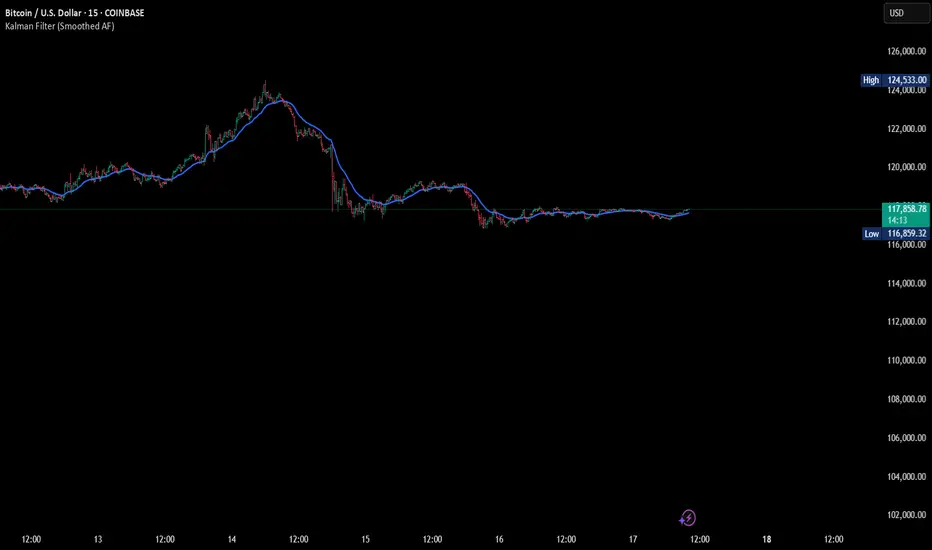
Kalman Filter (Smoothed)The Kalman Filter is a recursive statistical algorithm that smooths noisy price data while adapting dynamically to new information. Unlike simple moving averages or EMAs, it minimizes lag by balancing measurement noise (R) and process noise (Q), giving traders a clean, adaptive estimate of true price action.
🔹 Core Features
Real-time recursive estimation
Adjustable noise parameters (R = sensitivity to price, Q = smoothness vs. responsiveness)
Reduces market noise without heavy lag
Overlay on chart for direct comparison with raw price
🔹 Trading Applications
Smoother trend visualization compared to traditional MAs
Spotting true direction during volatile/sideways markets
Filtering out market “whipsaws” for cleaner signals
Building blocks for advanced quant/trading models
⚠️ Note: The Kalman Filter is a state-space model; it doesn’t predict future price, but smooths past and present data into a more reliable signal.
Ultimate Rejection BlocksThis indicator finds rejection blocks according to ICT concepts and marks out the equalibrium of the wick. Best used during killzone times and macro windows for top and bottom ticking.

Market Slayer Model 1.0This indicator only prints when a change in the state of delivery and breaker overlaps usually signaling a reversal if printed at the end of a swing high or swing low. Also added is standard deviation take profit projections which can be toggled on or off.
